
Abstract
Background:
Processes and systems are always subjected to faults or malfunctions due to age or unexpected events, which would degrade the operation performance and even lead to operation failure. Therefore, it is motivated to develop fault-tolerant control strategy so that the system can operate with tolerated performance degradation.
Methods:
In this paper, a reinforcement learning -based fault-tolerant control method is proposed without need of the system model and the information of faults.
Results and Conclusions:
Under the real-time tolerant control, the dynamic system can achieve performance tolerance against unexpected actuator or sensor faults. The effectiveness of the algorithm is demonstrated and validated by the rolling system in a test bed of the flux cored wire.
Introduction
With high demands on reliability, safety, and availability in industrial automation systems, fault-tolerant control (FTC) has been an important research topic during the last four decades. An early holistic view of FTC was given in Blanke et al., 1 and recent surveys and overviews were documented in Gao et al., 2 Yu and Jiang, 3 Zhang and Jiang, 4 and Yin et al. 5 FTC techniques are divided into passive FTC and active FTC. Compared with the passive FTC, the capabilities of which diminish as the number of fault scenarios increases, the active FTC is more flexible to deal with different types of faults. 6 Fault diagnosis methods can be categorized into model-, signal-, and knowledge-based methods. 2 As a possible solution to ensure safe and reliable operation of the system, the model-based fault detection and isolation (FDI) and FTC techniques have achieved fruitful results.7–12 The sliding mode control, 8 adaptive decentralized control, 9 and coprime factorization techniques 10 have been applied successfully. Youla parameterization–based FTC was developed in Ding et al. 11 and Yin et al. 12 to solve a nonlinear system.
Modern automation industries enable the availability of a large amount of historical data. As a result, data-driven modeling, diagnosis, and FTC have become a hot research topic. Data can be used for learning to extract the knowledge base such as using fuzzy approximation, 13 neural network (NN)-based methods, 14 K-clustering, 15 and support vector machines (SVM).16,17 Moreover, fault feature can also be exploited from the collected data, such as using principal component analysis (PCA),18,19 empirical mode decomposition (EMD),20,21 and so forth.22–25 It is the performance indicators (PIs) that are very important in the industrial process. Both sensors and control system will target on the plant to obtain the benefits of maximization by optimizing the performance indicator within the scope of safety. FTC is a good alternative that has the capability of approaching to performance indicator without any fault by adjusting the system variables. In Yin et al., 12 a gradient-based optimization method was given to optimize the system performance by means of disturbance rejection. In Macgregor and Cinar, 22 a recursive total principle component regression (R-TPCR)-based design and implementation approach was proposed for efficient data-driven FTC and optimization.
Strongly motivated by keeping the performance indicator fault free, it is of interest to seek an FTC approach in order to preserve the normal performance indicator under all kinds of unexpected fault scenarios. The performance indicator without any fault is a reflection of the system’s real ability and easy to be gained from the obtained data. However, it becomes a challenge in the case of fault because the unexpected fault has changed the maps of system states and made the original controller unavailable; meanwhile, there are not enough valid data to develop an FTC controller for an early fault. Reinforcement learning provides an inspiration to solve the above problem. Reinforcement learning is about learning from the interaction on how to behave in order to achieve a goal.26–28 The reinforcement learning agent and its environment interact over a sequence of discrete time steps and gain a series of optimal actions finally. If an unexpected fault is considered as the environment, and the performance of the system under fault-free condition is regarded as the desired goal, the controller can be designed by reinforcement learning to achieve the optimal behavior. In this paper, a novel structure of FTC is proposed based on reinforcement learning, and the advantages are given as follows:
This approach is a data-driven method without knowing the mechanism model of plant;
This approach is an online method which is suitable for unexpected faults without prior fault information;
The controller has the ability to take optimal actions to mitigate the adverse influences from faults.
Problem description and preliminaries
Problem description
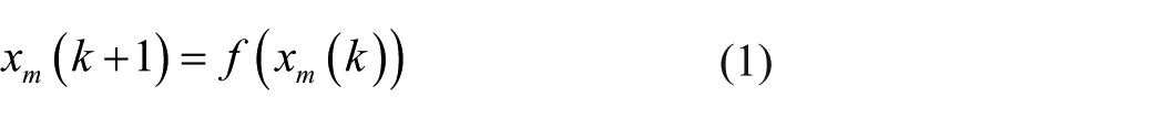
Suppose a time series of the plant
The addressed FTC system is composed of three units: the plant, the reference model, and the fault-tolerant controller. The plant works well under fault-free condition with a pre-designed controller, which is represented as a form of time series of the data
Reference model
For a system, the reference model can be expressed in the form of
where
There are various methods for system identification such as least square method (LSM), maximum likelihood method (MLM), and NN. A reference model can be obtained using the data of the time series of the plant under fault-free condition, as depicted in Figure 1.
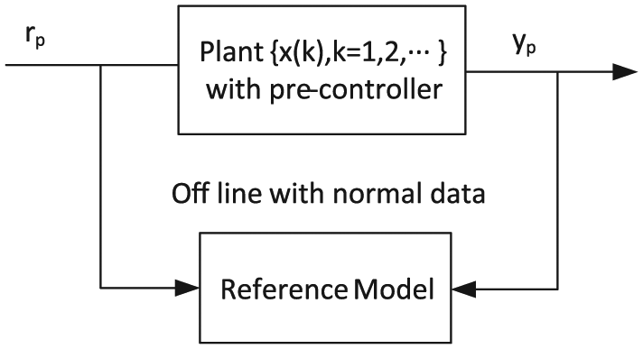
Obtaining the identification for the reference model.
Performance index
The stage costs
where
The stage costs
where
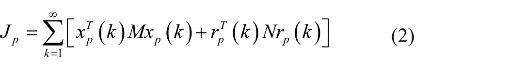
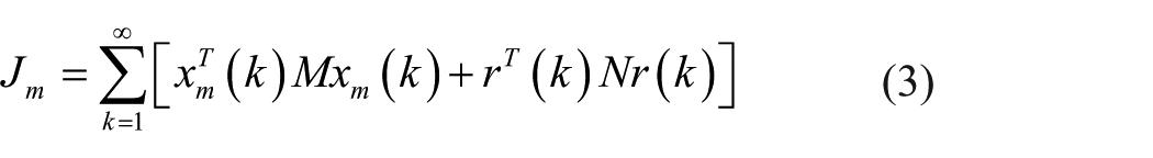
Define the performance index
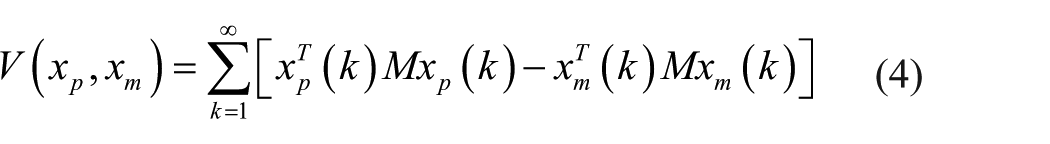
and the performance index
It is obvious when
Remark 1
The stage costs
Under faulty condition, one can regulate the real-time states/outputs by tracking the reference model performance using learning algorithms.
Reinforcement learning method
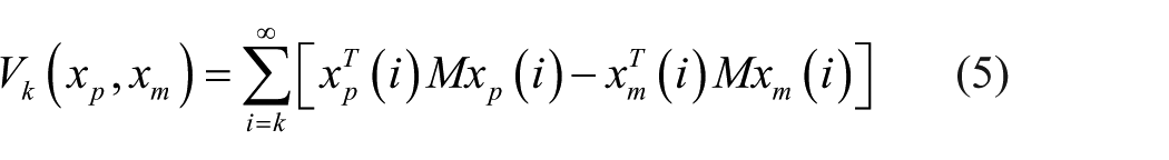
In fact, it seems that we know little about real-time dynamics after the fault occurs. The traditional controllers often struggle to provide an effective control due to the lack of information on real-time dynamics. The reinforcement learning that is motivated by statistics, psychology, neuroscience, and computer science is a powerful tool to deal with uncertain surrounding by interacting with its environment. As in Bhatnagar and Babu, 29 Watkins and Dayan, 30 Sutton and Barto, 31 Bradtke and Ydstie, 32 and Ngia and Sjoberg, 33 the basic theory and methods of the reinforcement learning are simply introduced here. The basic frame of reinforcement learning is shown in Figure 2. 26
A basic frame of reinforcement learning.
An agent will get the evaluation of good or bad behavior on the environment and learn through experience without a teacher who teaches how to do. In each training session, named episode, the agent explores the environment by changing action
Consider a Markov decision process
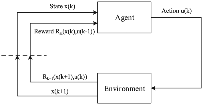
The value of a policy
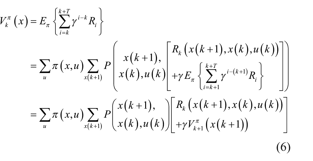
where
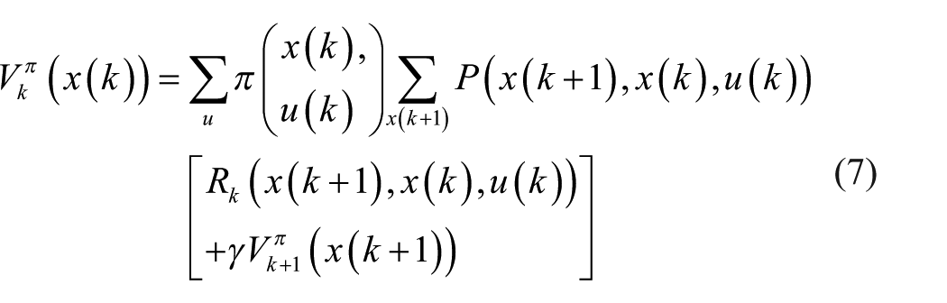
Therefore, the optimal actions can be gained by alternating the value iteration (equation (8)) and policy iteration (equation (9)) according to the following two equations
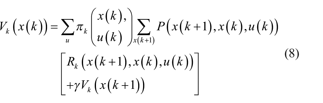
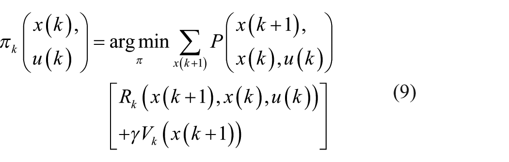
where
To a deterministic system
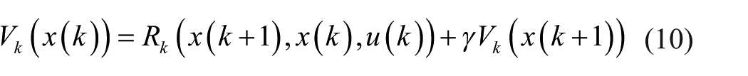
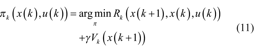
There is only state information in formulae (10) and (11). One can obtain the optimal action only using the current state, but without knowing the system dynamics.
S Bradtke and BE Ydstie 32 presented the stability and convergence results for dynamic programming–based reinforcement learning applied to linear quadratic regulation. Here, reinforcement learning is used to design a tolerant controller for systems subjected to faults.
Reinforcement learning–based FTC design
Reinforcement learning–based FTC
The first thing to apply in reinforcement learning is to determine the cost function
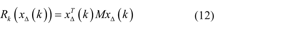
The function
where
As a result, we have
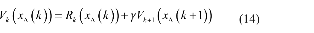
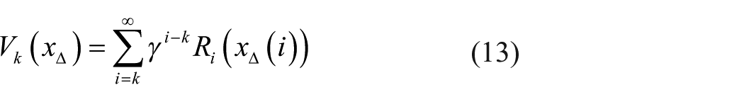
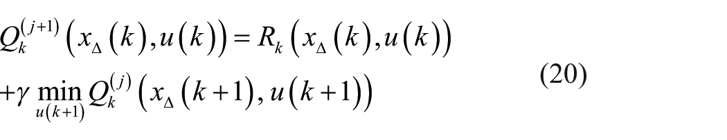
Following the Bellman optimal equation,29–31 the optimal value function
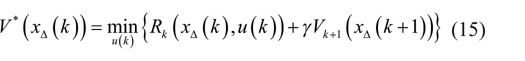
where
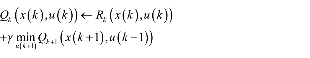
It is noticed that equation (15) cannot be used online because one cannot know the cost function of the future time, that is,
The evaluation function
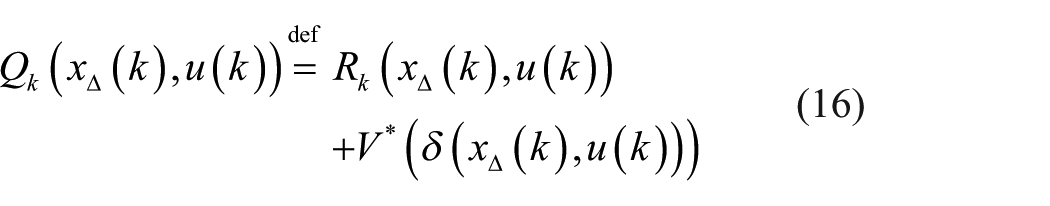
where
If
Denote the optimum of
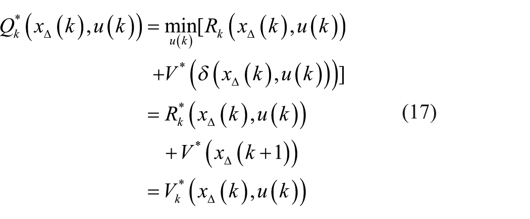
where the superscript * expresses the optimal values.
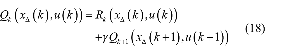
It is seen from formula (17) that
The policy iteration formula (11) of a deterministic system is transformed to formula (19)
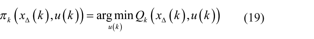
The optimal action
The policy evaluation is to find the optimal value in the case of current policy
The policy improvement is to find another policy that is better, or at least no worse according to equation (19) by greedy method.
The alternation procedures are given as follows 31
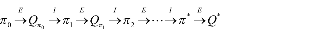
where E and I are the policy evaluation and policy improvement,
It is important for the iteration to be convergent, and the convergence of the Q learning for deterministic Markov decision process (MDP) is given in Sutton and Barto, 31 shown as follows:
Lemma 1
Consider a Q learning agent in a deterministic Markov decision process MDP with bounded reward
initializes its
Remark 2
Lemma 1 provides a guarantee on convergence of reinforcement learning–based FTC. Using policy iteration which includes alternation procedures of policy evaluation and policy improvement, the Q learning agent will finally converge to the steady state and control π*(x(k), u(k)) can be obtained readily.
Performance index compensator
The fault-tolerant reinforcement learning-based (RL) controller π*(x(k), u(k)) has the capability of approaching to healthy performance index within its ranges. If the reinforcement learning-based controller (RLC) cannot achieve the goal of performance index, for instance, due to the actuator saturation, the compensator will enhance the FTC performance. The schematic block diagram with compensator is depicted in Figure 3.
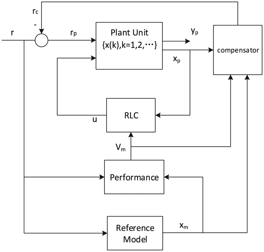
The schematic block diagram with compensator.
The reference model works parallel to the plant unit and yields the healthy state variable
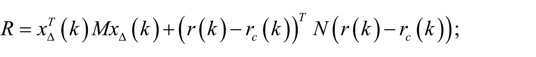
Denote by ∆J the error between the stage costs
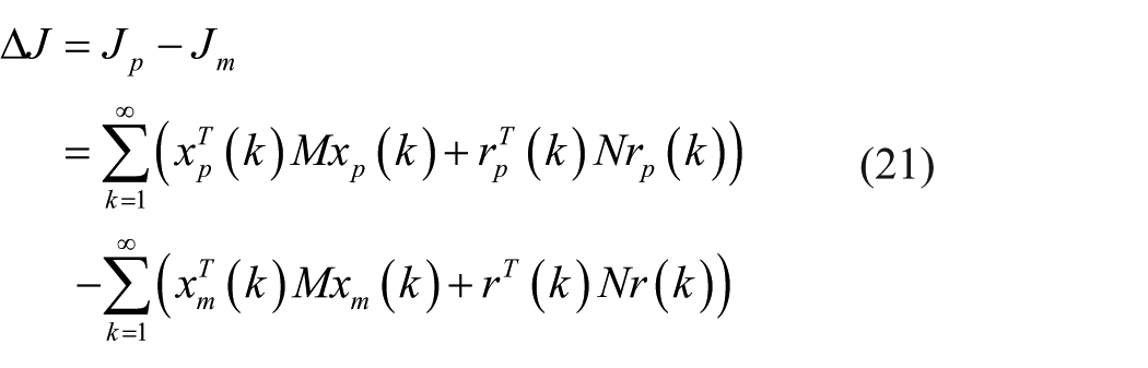
From Figure 3, one can have

Substituting equation (22) into equation (21), one has
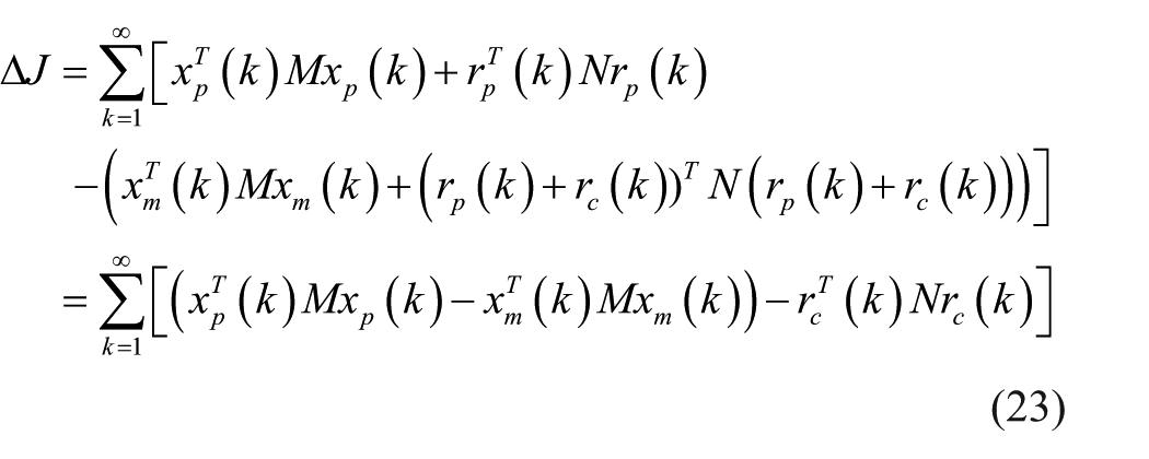
Substituting
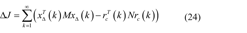
For an online system, what we focus on is the error ∆J (k) of the performance index at every sampling time

Letting

There exists a nonsingular matrix

where
Based on equations (26) and (27), one has

Let

where
As a result, equations (28) and (29) imply

Suppose that the first item is determined to compensate; therefore,
From equation (30), we can have
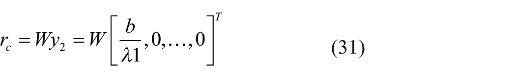
Remark 3
Equation (31) is a special solution of equation (26), which means
A compensation
The compensation aims to make the performance index of the real-time system under faulty conditions track the performance index of the reference model.
In the fault-free case,
The reinforcement learning-based fault tolerant control (RL-FTC) algorithm can be summarized as follows:
Step 1. Calculate x∆(k) according to x∆(k) =
Step 2. Initialize
Step 3. Select an action
Step 4. Compute the compensation
Step 5. Receive immediate reward
Step 6. Observe the new state
Step 7. Set the next state
Step 8. Find the best action π* according to the formula (19);
Step 9. Repeat Steps 5–8 until it is convergent.
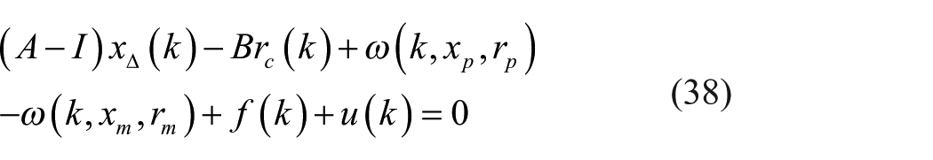
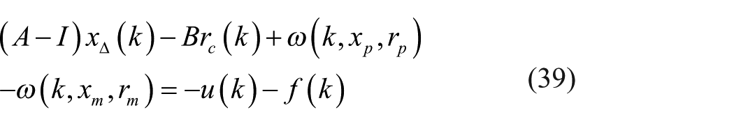
Further analysis on compensation
Actually, the proposed FTC method does not need any detailed information on the system dynamics. However, for the purpose of further analysis, we adopt the model expression to the theoretical analysis and assume that the time series of the plant can be described by the following discrete time form
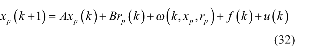
where

It is noticed that
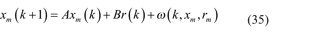
The reference model dynamics can be extracted as follows
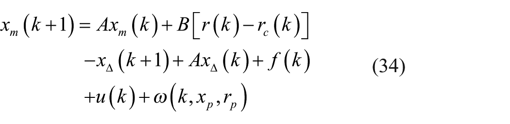
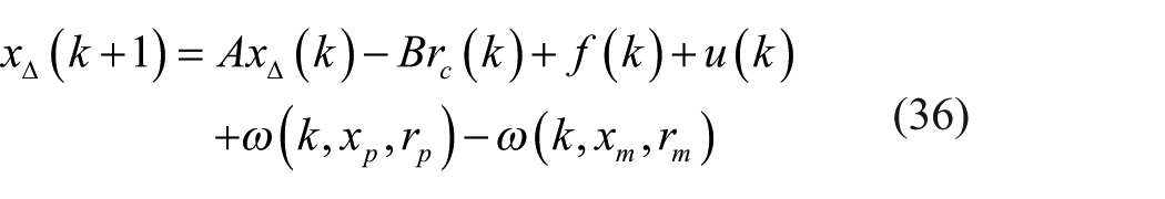
Therefore, from equation (34), we can have
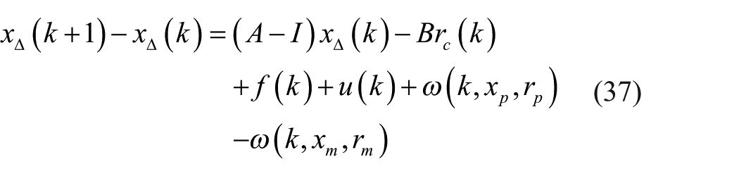
Subtracting x∆(k) from both sides of equation (36), one has
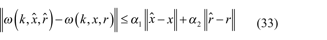
If
then one has
Furthermore, one has
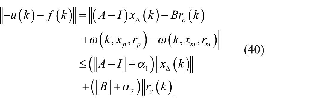
which is equivalent to
As a result, there is
Clearly,
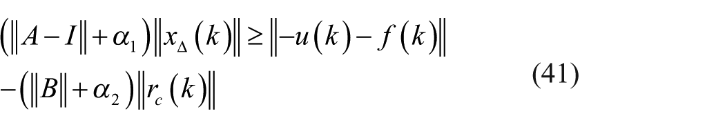
Remark 4
The inequity (equation (42)) indicates that a controller
When comparing equation (42) with equation (43), it is clear that
Experimental results
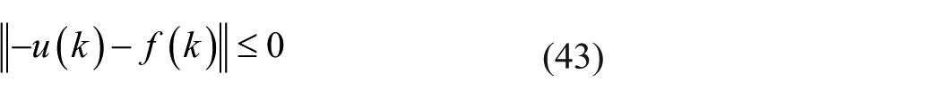
Flux cored wire, also called tubular welding wire, is an important welding material that is used for different applications by adjusting alloy composition and type. The process scheme is shown in Figure 4. First, the raw steel strip of pay-off machine is preprocessed by washing and drying. After that, the post-processed steel strips that are mixed up with the given powder using the powder feeding servo system begin to roll. After several rolling stages, the flux cored wires are produced. Finally, they are synchronously collected as the product by a wire winding machine. All the processes are controlled by the computer control system. There are some restrictions in the production process for flux cored wire such as the maximum tension of 0.4 mm/m and the error of powder content should be equal to or less than 1%. These performance criteria are realized by quality speed control. False or mistakes may cause wire break or quality rejection.
The system scheme of flux cored wire.
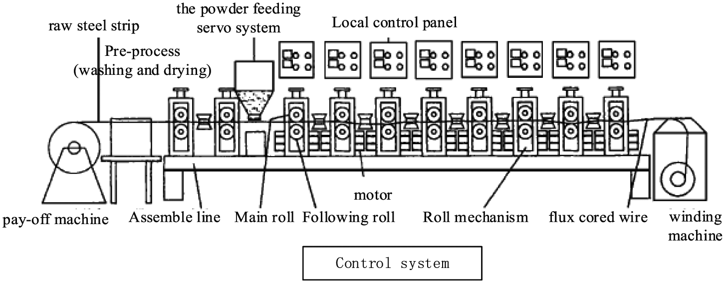
We focus on the rolling system because it is the core of the system. Moreover, we also abandon the preprocessing and the powder feeding servo system because they have little influence on the rolling system. The rolling system consists of a driven subsystem by several gear motors and an oppression subsystem that has an independent control system which provides proper pressing force according to tension detection. The oppression subsystem is considered as a disturbance to the driven subsystem for the target of speed control in the flux cored wire process. Therefore, the oppression subsystem is not considered in our test. The test bed of flux cored wire shown in Figure 5 is driven by four AC motors (M1, M2, M3, and M4) with a MultiQ PCI Data Acquisition board, a control board, and a data acquisition and control board (DACB) interface board from Quanser. The character of test bed depends on the AC motors. Every single motor has its independent control channel in order to imitate a split drive-type system. All motors work well by the proportional–integral–derivative (PID) speed output feedback in the healthy state and the rollers also operate well.
Test bed of flux cored wire.
The motor M4 is selected to test our approach under the condition that the motors M1–M3 operate normally. The motor M4 within a range of 0–2000 r/min is driven by a frequency transformer with a control input of voltage. The computer provides a controllable speed range of ±250 r/min which converts to the voltage signal of −5 to 5 V by an analog conversion channel from Quanser. The target of the driven subsystem is to keep the roller rotational speed

where

where ∆J is the performance index that indicates the difference of the roller speed between
For a flux cored wire system, the reference speed
A period from 60 to 80 is selected randomly to test the effect of FNN. The estimated states by FNN and the original healthy data are shown in Figure 6. The blue line represents the original data and the red line represents the output of NN. The estimated states by FNN is consistent with the original data.
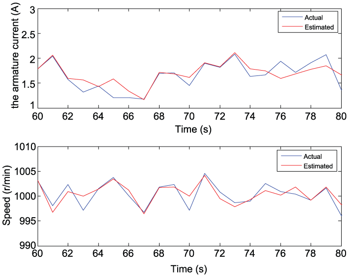
The estimated states by FNN and the actual state data (from 60 to 80).
The estimated states by FNN and the original healthy data of another period from 600 to 620 are shown in Figure 7. One can see that the two curves show good consistency. Therefore, the well-trained FNN can be used as a black box reference model.
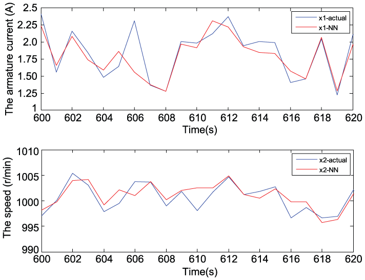
The estimated states by FNN and the actual state data (from 600 to 620).
FTC: sensor fault scenarios
A speed step fault with an amplitude of 180 r/min
A step fault of speed sensor with an amplitude of 180 r/min that is within the controller’s regulations added to the control system with the sampling number of 1000. The controller is designed by reinforcement learning and its output is
Figure 8 shows the evolution of error ∆J of the performance indices. The curves with and without control coincide before a fault occurs. Without tolerant control, one can see that the performance index has a significant difference after the fault occurs. Conversely, with tolerant control, the performance indices derive small errors after the fault occurs. The RL learning control is shown in Figure 9. Compared with the scenario without the RL control, the performance index has been improved much. The system states are shown in Figure 10. It is seen from Figure 10 that FTC can mitigate the adverse influences from the faults, which can be seen more clearly for the motor speed.
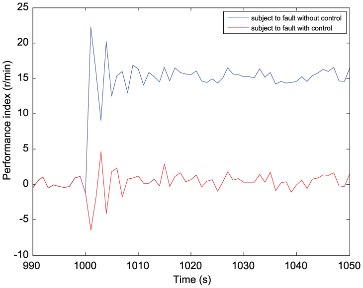
The error ∆J of the performance indices.
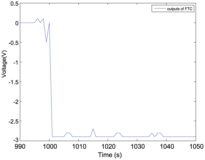
The output of RL controller.
State evolution.
A speed step fault with an amplitude of 600 r/min
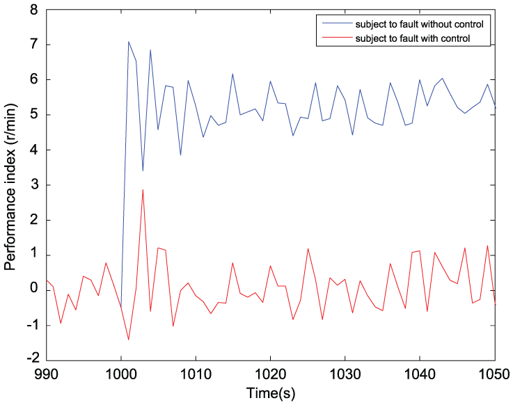
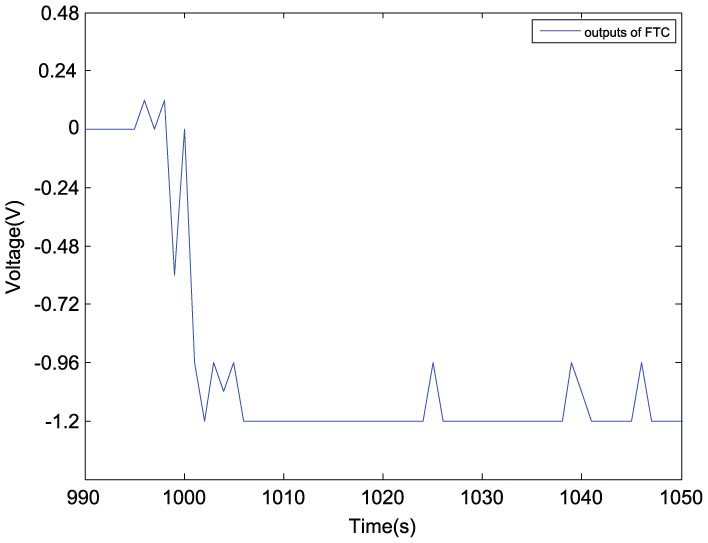
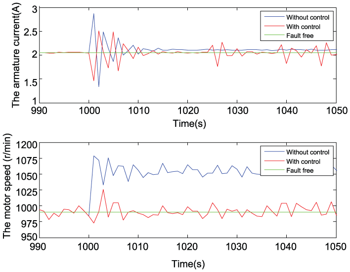
The amplitude of the fault is enlarged to 600 r/min which means that it is out of the range of the controller, that is, 250 r/min. The error ∆J of the performance indices, the output of RLC, and the state evolution are shown in Figures 11–13, respectively. From Figure 11, one can see that the steady error ∆J values of the performance indices are, respectively, 50 (red curve: without control) and almost 0 r/min with fluctuation (blue curve: with control). From Figure 13, one can see that tolerant control can make the motor speed recover from 1600 down to 1000 r/min after the fault occurs.
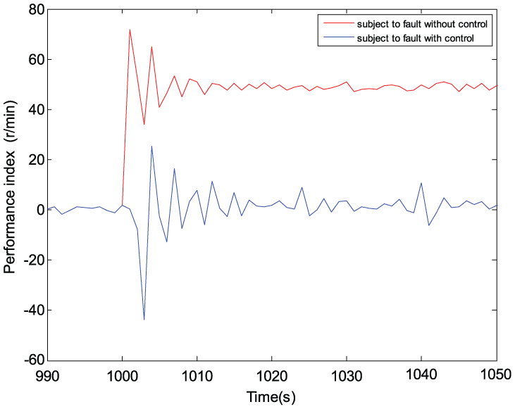
The error ∆J of the performance indices.
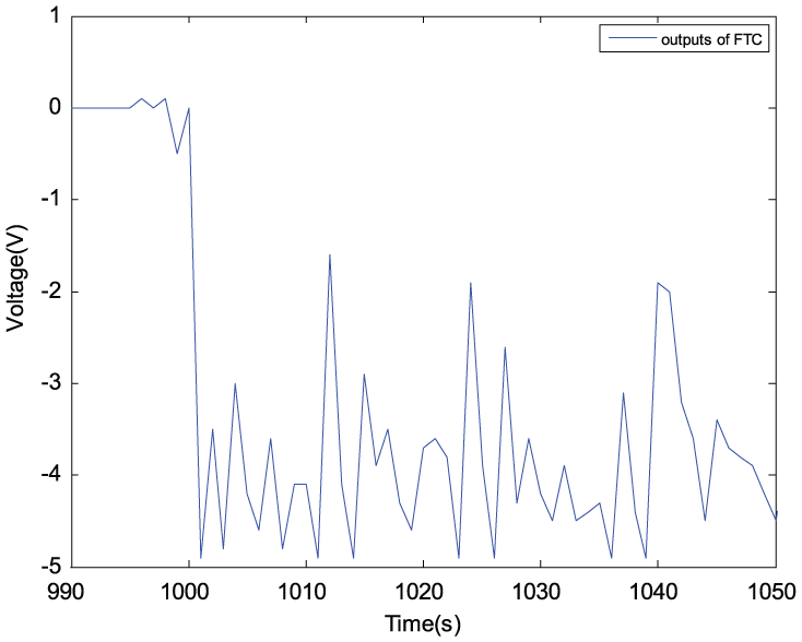
The output of RL controller.
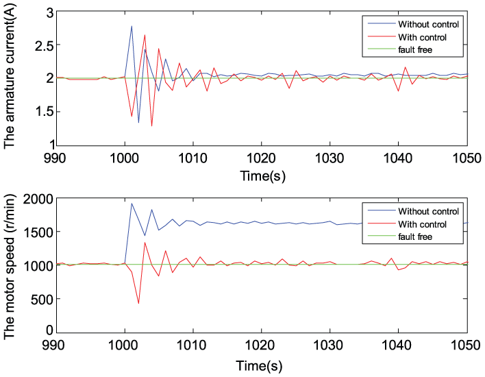
State evolution.
FTC: actuator fault scenario
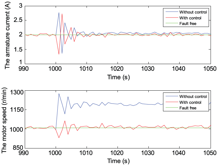
An error of speed actuator with an amplitude of 60 r/min is also tested (the control signal has the voltage of 1.2 V). Figure 14 shows the evolution of error ∆J of the performance indices, implying a better performance index with RL control than without control. The output of RL controller is shown in Figure 15. The state evolution is depicted in Figure 16. With the function of RL learning control, the motor speed is keeping the trace fault free (red line and green line) compared to the motor speed without control (blue line) when a speed actuator fault occurs. The armature current without any load changes is also keeping stable except suffering a transient process caused by the disturbance of actuator false.
The error ∆J of the performance indices.
The output of RL controller.
State evolution.
Conclusion
The reinforcement learning is a data-driven online method which directs to the goal by iterating value evaluation and policy improvement, which can achieve an optimal action without knowing any system dynamic characteristics that are difficult to know at the beginning when a fault occurs. In this paper, we have shown that reinforcement learning is an effective approach to solve the FTC problem when the faulty information is unavailable to the designers. The proposed reinforcement learning–based FTC controller has been applied to a flux cored wire system, and the effectiveness has been well demonstrated. It is worthy to point out that the proposed FTC is real-time RL learning with the aid of the reference model to track the performance index without any fault. The reference model was identified by FNN instead of difficult mechanism modeling. As a result, the method used is data driven in essence. If an explicit reference model cannot be obtained for a complicated system, an implicit model could be obtained by data-driven learning which can be used as the reference. It would be of interest to develop a reference model–free data-driven FTC algorithm at the cost of the system performance in the future.
Footnotes
Declaration of conflicting interests
The author(s) declared no potential conflicts of interest with respect to the research, authorship, and/or publication of this article.
Funding
The authors would like to acknowledge the research support from China Scholarship Council, the Alexander von Humboldt Renewed Stay Fellowship, and the E&E faculty at the University of Northumbria.