Sage Journals: Discover world-class research

Abstract

This paper deals with the eddy current technique for nondestructive evaluation of the crack depth on a massive specimen used in aeronautical industry. A set of C-scan eddy current images is analyzed to reduce the noise and to select suitable features, which can be used to estimate the crack depth. Based on this study, a method relying on polynomial forward models of the relationship between crack depth and the maximum value of the sensor impedance is proposed. The least square and the non-negative least square techniques are applied to analyze the usability of proposed models. The error of obtained estimations is smaller than 10%, for almost used experimental data.

Keywords

Non-destructive evaluation eddy currents multi-frequency approach behavioral multi-frequency forward model

Introduction

The non-destructive evaluation (NDE) of metal massive structures by eddy current (EC) technique is widely considered in industry. It allows characterizing defects^1–3 or evaluating physical parameters under certain conditions^4,5 with sufficient accuracy. However, it is still an “ill-posed” problem and limited in applications^6,7 due to the difficulty of feature extraction and the complex of algorithm of inverse problem solution.

Among the published studies, there are a lot of efforts to solve the qualitative analysis problem. For this field of study, the pulsed eddy current (PEC) techniques are widely used. In many researches, the time domain and the frequency domain features of PEC sensors are extracted and analyzed to detect and characterize cracks.^3,8–10 Recently, there are many reports on the PEC thermography technique. Most of them aim to detect and localize cracks in different structures and materials, for example, in alloy plates,¹¹ in ferromagnetic materials,^12,13 in aeronautical structures,^14,15 or in carbon fiber–reinforced plastic.^16,17 Many other works focus on the improvement of the defect detection efficiency through the improvement of feature extraction or image processing algorithms. These approaches can be used to sizing surface or subsurface cracks on various types of metal plates.^18–22

However, for quantitative crack estimation, to our knowledge, there are not many publications. The work implemented by Cheng et al.²³ aims at the determination of crack depth using a polynomial direct model and also a neural network. The signal features used in this case are exploited from an A-scan, which means that the sensor makes measurements along a line positioned vertically on the defect. The characteristic of signals which are used to estimate crack depth is their amplitude. These studies concern NDE structures with relatively large electro-eroded cuts (a few millimeters). A thesis carried out in SATIE laboratory (France) by Ravat²⁴ also discussed the dimension estimation of electro-eroded defects using EC. The author proposes an algorithm which gives quite good results on sub-millimeter cuts, but the case of real cracks has not been studied. It is a single frequency approach, wherein the nine parameters relating to the form of EC signal in impedance plane, and two hybrid parameters obtained by combining these parameters, are used to construct a direct model. This model consists of a system of two non-linear equations with two variables: the length and depth of the crack. These two variables are estimated by solving the system of equations. Another work implemented by Yusa et al.²⁵ aims at designing an uniform EC probe with 23 arrayed detection elements and proposing an approach to estimate the surface crack depth using the developed probe. The depth of crack was estimated using a computational inversion method based on the k-nearest neighbor algorithm. Some real mechanical fatigue cracks with the depth of 1.1, 2.1, 5.5, 6.7, and 8.5 mm were used to test the method. The estimation results were 0.9, 1.9, 3.8, 4.3, and 5.7 mm, respectively.

In this paper, we consider a problem of estimation of crack depth sited on the surface of a massive structure. Our problem can be considered as an imaging problem as we have the impedance maps, obtained using absolute and differential EC sensors in C-scan mode for acquiring data. These sensors operate at two different frequencies. From the experimental images with real cracks, a processing procedure was implemented to reduce the affection of noise, to extract the appropriate features which can be used to estimate the crack depth. The depth is small, typically in the range from 200 to 800 µm. To solve the estimation problem, we propose to build a multi-frequency behavioral forward model by analyzing the relationship between impedance of EC sensor and the crack depth. The paper is organized as follows: section “Problem formulation” reports on the experimental setup and the problem formulation. In section “Processing and feature extraction of sensor impedance images,” we present the processing and feature extraction of impedance images. A model-based inversion method and the crack depth estimation technique are presented and discussed in sections “Model-based inversion” and “Crack depth estimation,” respectively. Finally, some conclusions to our work are given in section “Conclusion.”

Problem formulation

To address the problem of estimating depth of cracks in massive parts, the experimental data on which we rely were C-scan EC of the surface of massive specimens which have actual opening cracks. Each point of image, or pixel, corresponds to a position of sensor at which we have the complex value of sensor impedance.

To collect the data, two EC sensors operating on two different modes were used: an absolute sensor operates at the frequency of 500 kHz and a differential sensor operating at 400 kHz (Figure 1).

Figure 1.

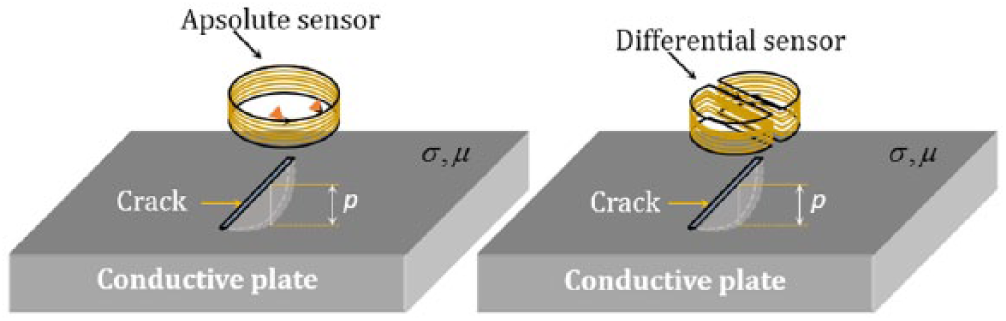
Illustration of the problem of estimating the depth of cracks on the surface of an electrically conductive target using eddy current method.

Data are collected from eight electrically conductive specimens that have worked in mechanical fatigue (Figure 2). These specimens were divided into two groups with four specimens in each group. The difference between two groups is the way that cracks were initiated (the shape of the used punch; Figure 2). So, for each group, the shape and the development of cracks are different.

Figure 2.

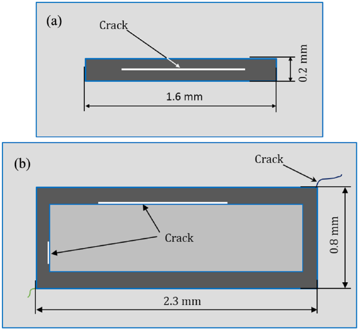
Top view of a piece in two groups of four pieces with the different type of crack initiation: (a) the first type of affected force: samples M11, M12, M13, and M14 and (b) the second type of affected force: samples M21, M22, M23, and M24.

The specimens of the first group are called under the names M11, M12, M13, and M14, those in the second group are M21, M22, M23, and M24 (Figure 2).

Three EC measures (C-scan) were performed on the samples (conductive specimens) after three cycles of fatigue which they are suffered. The crack depth increases from one cycle to another. It is typically of 200, 400, and 800 µm at the end of three successive cycles. These depths are typical values, which means that they may have some differences between tested specimens (Figure 3). At the end of the third fatigue cycle, the tested specimens were cut to determine crack depths.

Figure 3.

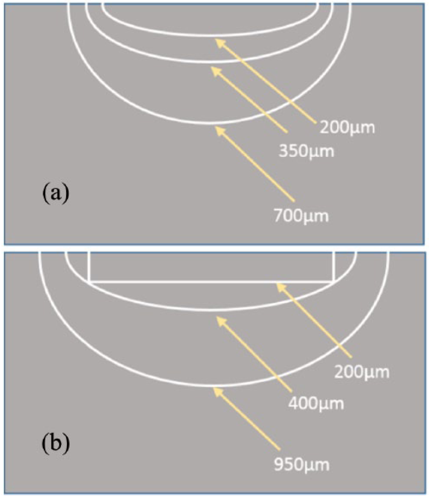
Section of specimens after three fatigue cycles: (a) cracks on the sample M13 under the first type of fatigue force and (b) cracks on the sample M24 under the second type of fatigue force.

The development of our method for estimating crack depth p consists of five steps. It carries, first, the noise treatment for images that have been provided to us, in order to reduce its affection. It then focuses on the analysis of the images and the determination of useful features allowing to estimate the (maximum) crack depth p. Then, once these parameters are identified, it involves the development of a polynomial direct behavioral model. Finally, based on this model, we propose a method for estimating the parameter p.

Processing and feature extraction of sensor impedance images

Reduction of the influence of noise existing at the edges of images

The images obtained by C-scan of an (absolute or differential) EC sensor on the tested surface are impedance of the sensor. Figure 4 shows an example of the real and imaginary parts of the impedance of an absolute sensor, measured on the sample M22 at the end of the third fatigue cycle.

Figure 4.

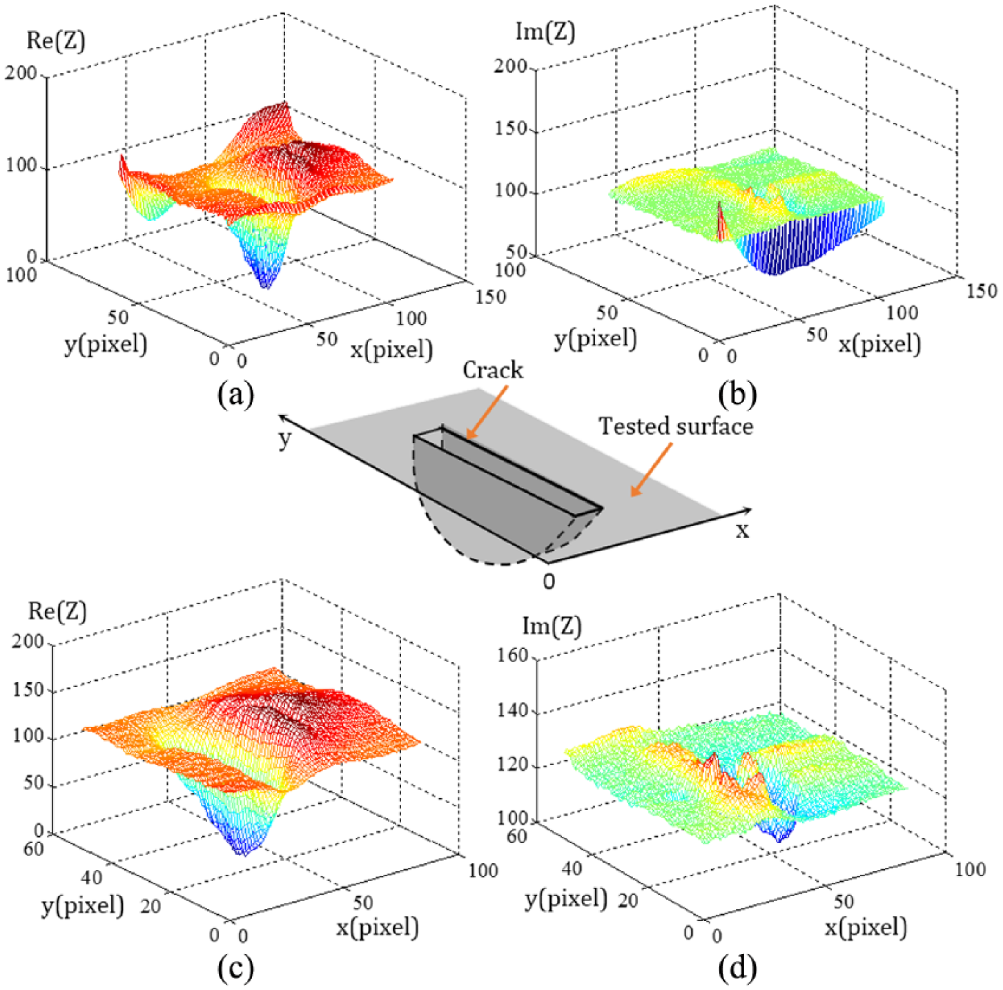
Image of the real part (a) and imaginary part (b) of the impedance of an absolute sensor measured on the sample M22 after the third fatigue cycle, and (c) and (d) are the real and imaginary parts after reducing the influence of noise at edges, respectively.

It is seen from Figure 4, as on all the measures, that the edges of the image contain significant noise. As the first treatment (noise reduction), we will simply remove some noisy lines at the border of images.

Subtraction of the complex image background

Besides that the images have a large noise at their borders, it can also be observed that the parts of the image which are outside of crack have their signal. They are steady and small, and so equivalent to a noise which we call background noise. Knowing that we are interested in only the representative signal of the crack, we will subtract the background noise from raw images (after noise reduction).

To do this, the background of the image, or the image of the background noise, is calculated from the lines located on the sides of the raw images. The background lines are calculated from the average value of several adjacent data lines and then the background of the images is created by interpolating the background lines. The obtained background noise image, thus, can be considered as the image that given by a C-scan on the same target in the case of the absence of cracks.

Figure 5 illustrates the modulus of the EC images after the subtraction of the background noise in the cases of using an absolute sensor and a differential sensor.

Figure 5.

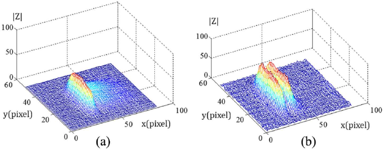
Image of the module of impedance of a sensor after subtraction of the background noise, carried out from the sample M13 after the third cycle of fatigue: (a) absolute sensor and (b) differential sensor.

Analysis and identification of interesting magnitudes in EC images

A first analysis of the images (treated as proposed in sections “Reduction of the influence of noise existing at the edges of images” and “Subtraction of the complex image background”) allowed us to see a clear link between the maximum value |Z_max| of the measured impedance module and the maximum depth p of the crack. This led us to study precisely the evolution of this magnitude as a function of p. We also study the relationship between the phase of Z_max and p as an extended parameter.

Estimation of |Z_max| and arg(Z_max)

After having identified the coordinates of the point of an image where the module of the impedance is maximum, knowing that this impedance value may be affected by noise, and in order to reduce its influence, |Z_max| is estimated as the mean value of the impedance module of nine adjacent pixels. As for the phase of the maximum impedance Arg(Z_max), it is also estimated as the average value of the impedance arguments of nine adjacent pixels.

With the absolute sensor, |Z_max| and Arg(Z_max) are unique. On the other hand, with the differential sensor, the image has two peak values. In principle, these two values are equal, but in practice they are slightly different due to the noise. For this type of sensor, we, therefore, take the decision to identify |Z_max| as the higher peak value. As shown in Figure 6, due to the noise, after two different cycles, the points {|Z_max|, Arg(Z_max)} (points marked in solid and no fill rounds in Figure 6), instead of being located in the same quadrant of the complex plane, are located in diametrically opposite quadrants. We correct this randomness by adding ±π to Arg(Z_max) so that the points {|Z_max|, Arg(Z_max)} obtained at the end of the different cycles are not in diametrically opposed quadrants, and so that the set of data is located in quadrants I and IV.

Figure 6.

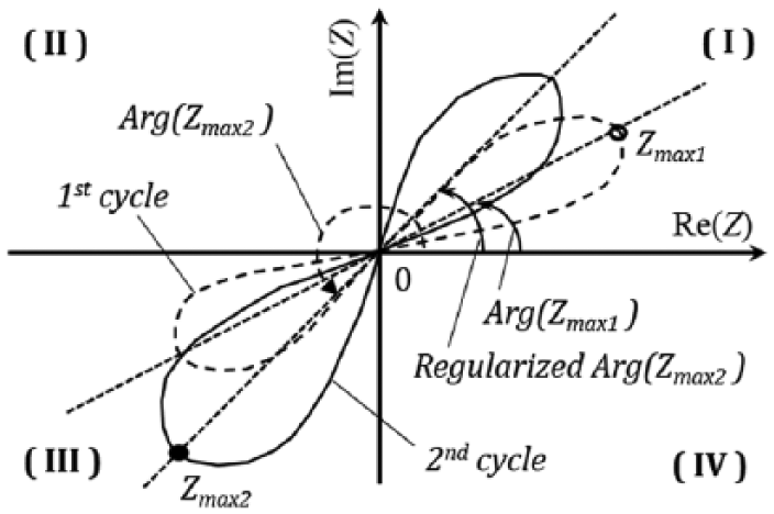
Illustration of Arg(Z_max) correction for the data of a differential sensor.

Behavioral study: evolution of |Z_max| and Arg(Z_max) as a function of p

The evolution of quantities |Z_max| and Arg(Z_max) as a function of p corresponding to the set of EC data obtained with an absolute sensor are shown graphically in Figures 7 and 8, respectively. Figures 9 and 10 represent data from the differential sensor.

Figure 7.

Relationship between |Z_max| and p. Data from an absolute sensor corresponding to the tested samples of (a) the first group and (b) the second group.

Figure 8.

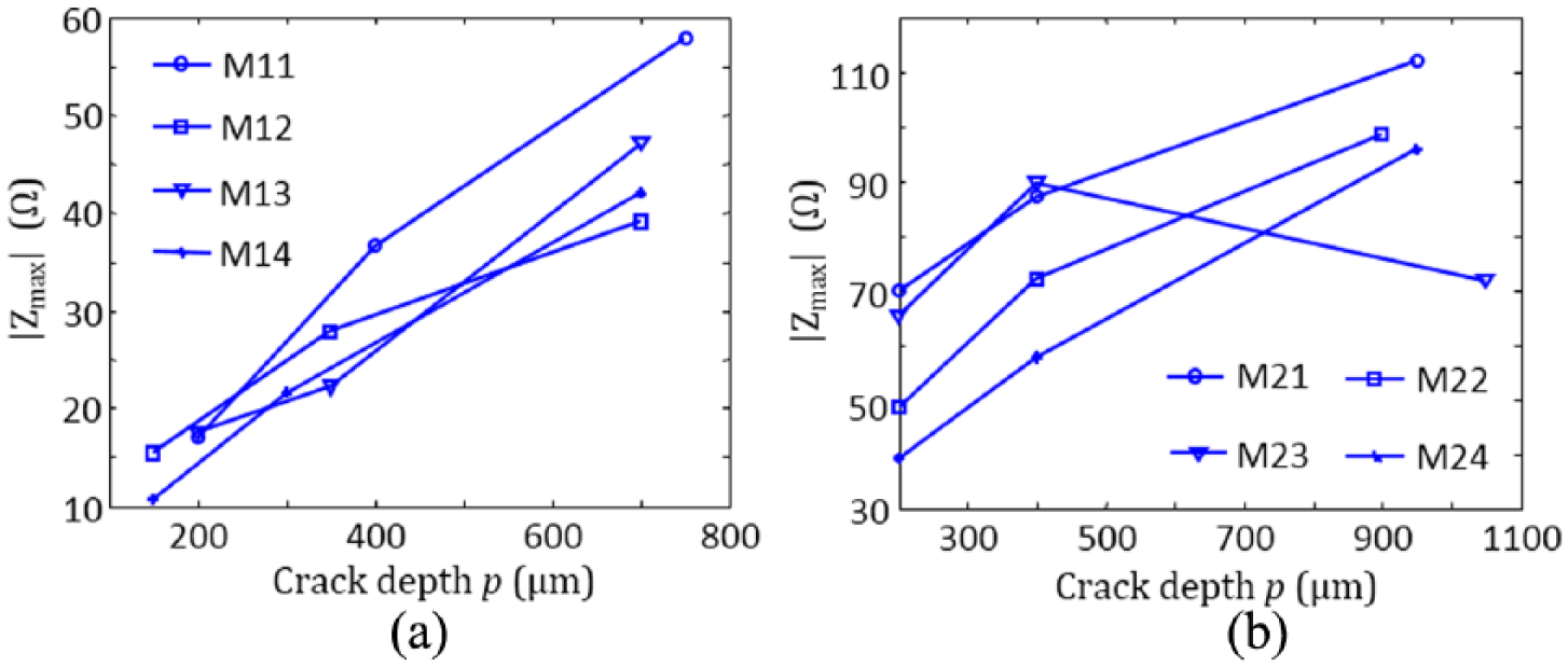
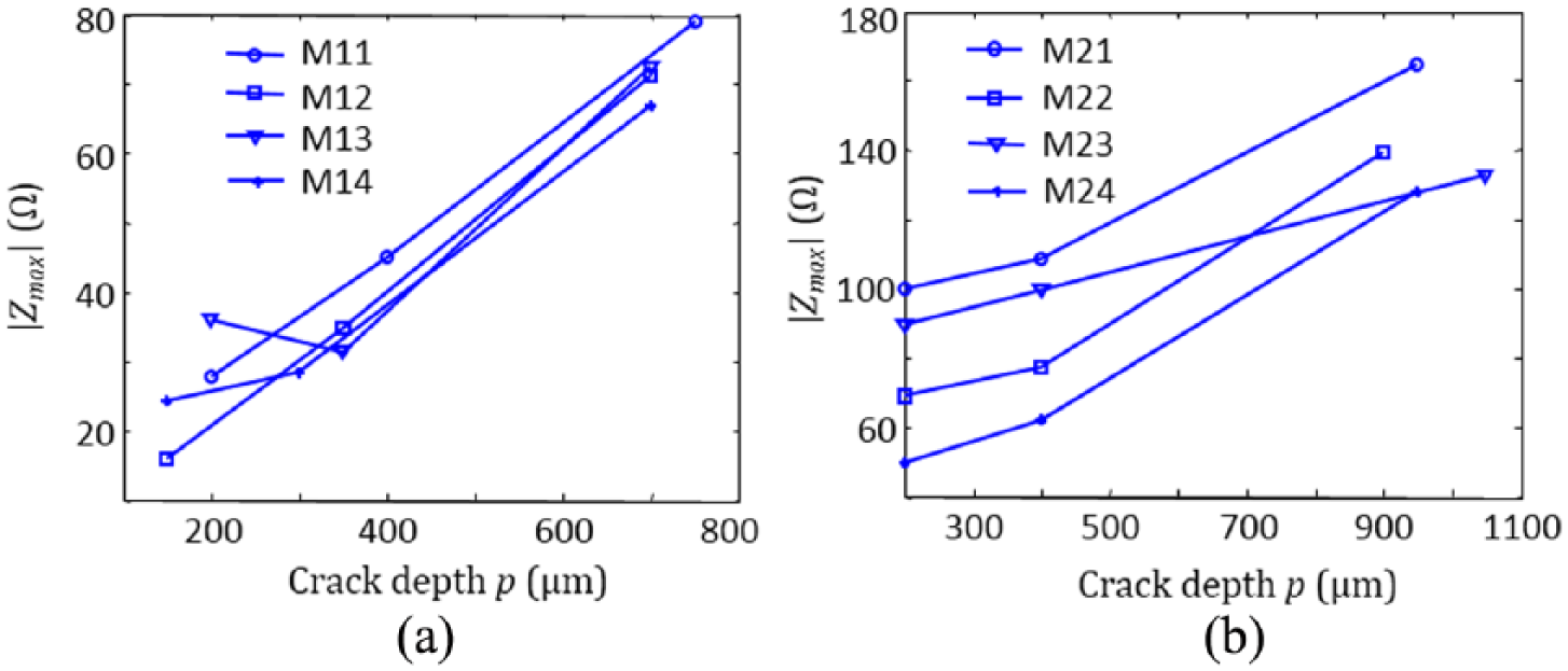
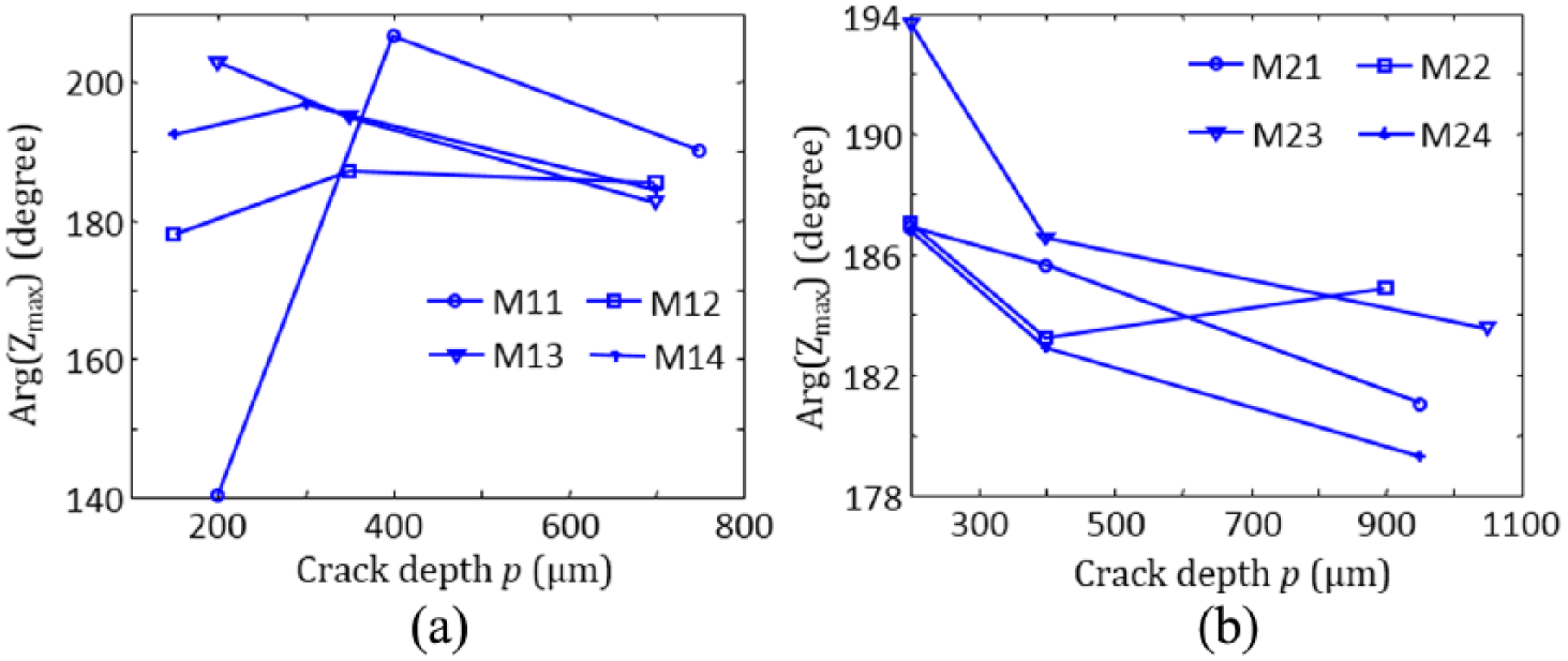
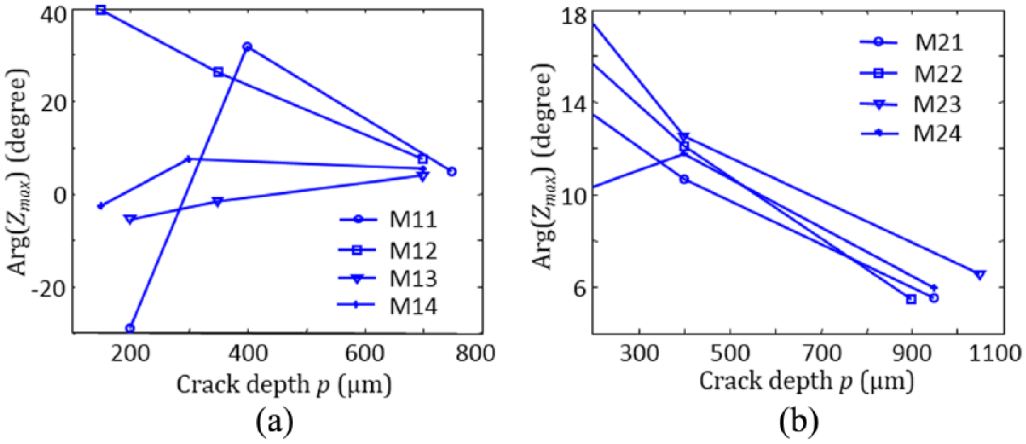
Relationship between Arg(Z_max) and p. Data from an absolute sensor corresponding to the tested samples of (a) the first group and (b) the second group.

Figure 9.

Relationship between |Z_max| and p. Data from a differential sensor corresponding to the tested samples of (a) the first group and (b) the second group.

Figure 10.

Relationship between Arg(Z_max) and p. Data from a differential sensor corresponding to the tested samples of (a) the first group and (b) the second group.

As far as the data from EC sensors are concerned, for the tested samples of the same group, from one sample to another, the impedance modules show a certain dispersion but their evolution follows the same trend. |Z_max| evolves monotonically (exception of M23 with absolute sensor and of M13 with differential sensor) increasing and non-linear. In addition, the data |Z_max| of the two groups are not in the same range of values. This leads us to establish different behavioral models for each of these groups.

As for Arg(Z_max) (p), within the same group of tested samples, its values present a certain dispersion and its evolution does not appear monotonous.

Model-based inversion

Polynomial direct model

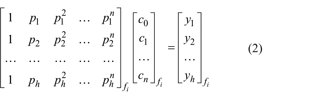
In this research, we propose to construct a polynomial direct behavior model for the NDE of massive pieces with cracks. The quantities to be modeled are |Z_max| and Arg(Z_max), and the parameter to be estimated (variable of the polynomial model) is the depth of cracks p. Let y be a quantity to be modeled (in this case it can be |Z_max| and Arg(Z_max)) at a certain frequency (500 kHz for the absolute sensor, 400 kHz for the differential sensor), a polynomial model of degree n of a quantity y as a function of p can be written

y = c_{0} + c_{1} p + c_{2} p^{2} + \dots + c_{n} p^{n}

(1)

Suppose that we have h magnitudes {y₁, y₂, …, y_h} at different frequencies f_i corresponding to h values of p. From these measurements, the formulation (1) of the direct model can be written under matrix relation (2)

{[\begin{matrix} 1 & p_{1} & p_{1}^{2} & \dots & p_{1}^{n} \\ 1 & p_{2} & p_{2}^{2} & \dots & p_{2}^{n} \\ \dots & \dots & \dots & \dots & \dots \\ 1 & p_{h} & p_{h}^{2} & \dots & p_{h}^{n} \end{matrix}]}_{f_{i}} {[\begin{matrix} c_{0} \\ c_{1} \\ \dots \\ c_{n} \end{matrix}]}_{f_{i}} = {[\begin{matrix} y_{1} \\ y_{2} \\ \dots \\ y_{h} \end{matrix}]}_{f_{i}}

(2)

We pose

\begin{array}{l} X_{f_{i}} = {[\begin{matrix} 1 & p_{1} & p_{1}^{2} & \dots & p_{1}^{n} \\ 1 & p_{2} & p_{2}^{2} & \dots & p_{2}^{n} \\ \dots & \dots & \dots & \dots & \dots \\ 1 & p_{h} & p_{h}^{2} & \dots & p_{h}^{n} \end{matrix}]}_{f_{i}}, c_{f_{i}} = {[\begin{matrix} c_{0} \\ c_{1} \\ \dots \\ c_{n} \end{matrix}]}_{f_{i}}, and \\ y_{f_{i}} = {[\begin{matrix} y_{1} \\ y_{2} \\ \dots \\ y_{h} \end{matrix}]}_{f_{i}} \end{array}

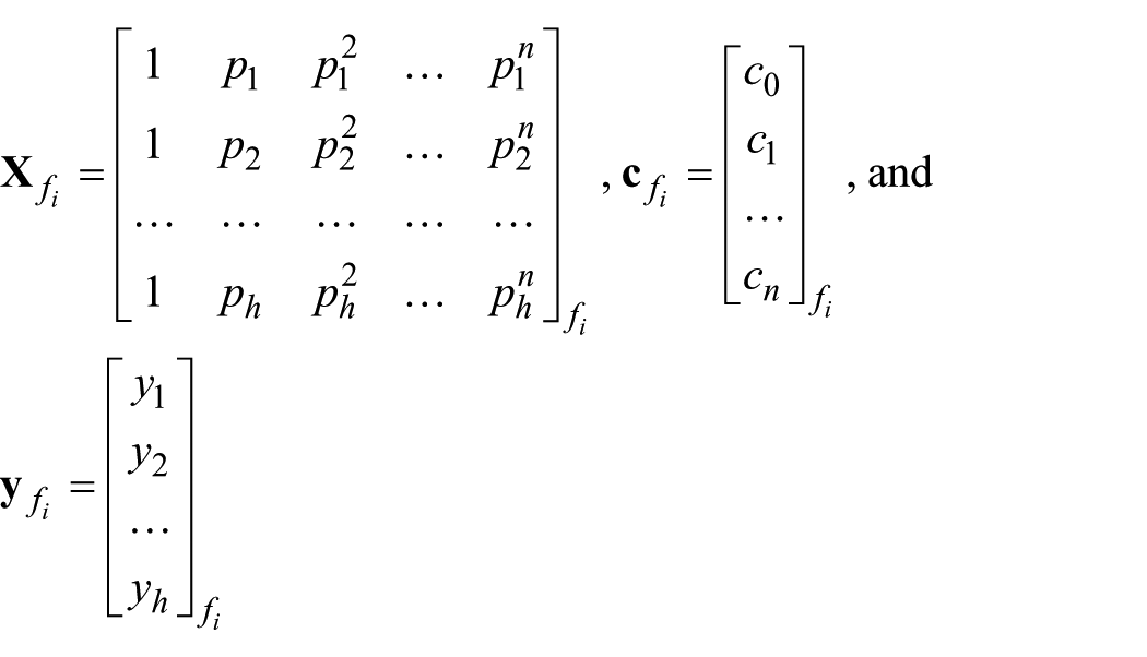
then equation (2) can be written as equation (3)

X_{f_{i}} c_{f_{i}} = y_{f_{i}}

(3)

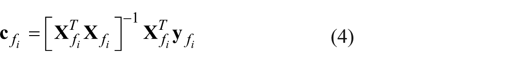
The coefficients of the polynomial model associated with a frequency f_i can be estimated by means of a least squares (LSQ) estimator

c_{f_{i}} = {[X_{f_{i}}^{T} X_{f_{i}}]}^{- 1} X_{f_{i}}^{T} y_{f_{i}}

(4)

LSQ and weighted least squares inversion procedure

Once we have a polynomial direct model connecting the parameter p to the quantities y that we are able to measure, we can solve inverse problem to estimate p from measurements.

For our NDE problem in this research, we can express in matrix form the relation between the measured quantities y and the depth p of cracks, in multi-frequency solution

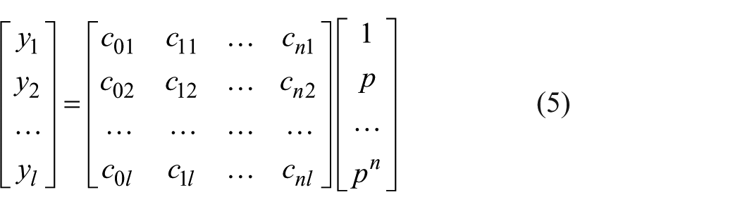
[\begin{matrix} y_{1} \\ y_{2} \\ \dots \\ y_{l} \end{matrix}] = [\begin{matrix} c_{01} & c_{11} & \dots & c_{n 1} \\ c_{02} & c_{12} & \dots & c_{n 2} \\ \dots & \dots & \dots & \dots \\ c_{0 l} & c_{1 l} & \dots & c_{n l} \end{matrix}] [\begin{matrix} 1 \\ p \\ \dots \\ p^{n} \end{matrix}]

(5)

where y_q, q ∈ {1, 2, …, l} are h quantities |Z_max| and Arg(Z_max) measured at different frequencies f_i, i ∈ {1, 2, …, k}, so that l = k × h. The c_jq, with j ∈ {1, 2, …, n}, are the coefficients of the polynomial model (of degree n), and p is the parameter to be evaluated. Equation (5) can also be written as

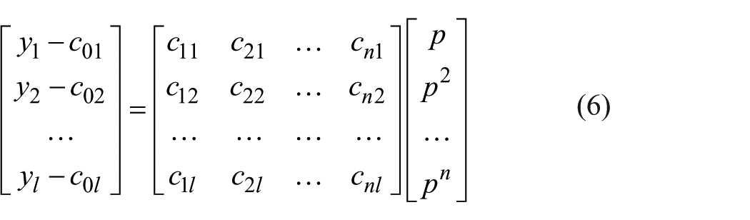
[\begin{matrix} y_{1} - c_{01} \\ y_{2} - c_{02} \\ \dots \\ y_{l} - c_{0 l} \end{matrix}] = [\begin{matrix} c_{11} & c_{21} & \dots & c_{n 1} \\ c_{12} & c_{22} & \dots & c_{n 2} \\ \dots & \dots & \dots & \dots \\ c_{1 l} & c_{2 l} & \dots & c_{n l} \end{matrix}] [\begin{matrix} p \\ p^{2} \\ \dots \\ p^{n} \end{matrix}]

(6)

By posing

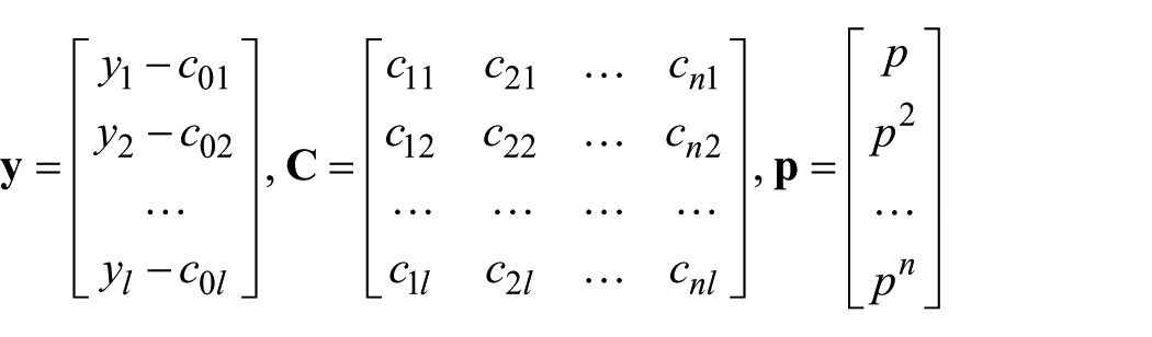
y = [\begin{matrix} y_{1} - c_{01} \\ y_{2} - c_{02} \\ \dots \\ y_{l} - c_{0 l} \end{matrix}], C = [\begin{matrix} c_{11} & c_{21} & \dots & c_{n 1} \\ c_{12} & c_{22} & \dots & c_{n 2} \\ \dots & \dots & \dots & \dots \\ c_{1 l} & c_{2 l} & \dots & c_{n l} \end{matrix}], p = [\begin{matrix} p \\ p^{2} \\ \dots \\ p^{n} \end{matrix}]

equation (6) can be written as

y = C p

(7)

Since y and C are known, the estimation $\hat{p}$ of the vector p can be obtained by LSQ technique (ordinary least square (LSQ) or non-negative least square (NNLSQ))

\hat{p} = {[C^{T} C]}^{- 1} C^{T} y = [\begin{matrix} \hat{p} \\ \begin{matrix} \hat{p^{2}} \\ \begin{matrix} \dots \\ \hat{p^{n}} \end{matrix} \end{matrix} \end{matrix}]

(8)

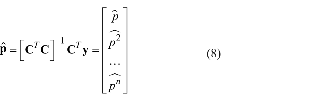
This operation makes it possible to estimate p by simply extracting the value $\hat{p}$ from the vector $\hat{p}$ , or taking into account all the elements of $\hat{p}$ , for example, by making an estimation by LSQ or weighted least squares (WLSQ) criterion.²⁶

The estimation $\hat{\hat{p}}$ can be receipted from the iterative calculation (9)

[\hat{\hat{p}}] = a r g \min_{(p)} [(\hat{p} - p) (\hat{p^{2}} - p^{2}) \dots (\hat{p^{n}} - p^{n})] Q [\begin{matrix} \hat{p} - p \\ \hat{p^{2}} - p^{2} \\ \dots \\ \hat{p^{n}} - p^{n} \end{matrix}]

(9)

where Q is a weight diagonal matrix. At each iteration, we change value of p (starting, for example, from $\hat{p}$ ), and the estimation consisting in choosing the value $\hat{\hat{p}}$ which minimizes the computed distance. In the case of an LSQ estimate, the weighting matrix is unitary (Q = I). In that of an estimation by WLSQ, Q is the following diagonal matrix

Q = d i a g (\frac{1}{{(\hat{p})}^{2}} \frac{1}{{(\hat{p^{2}})}^{2}} \dots \frac{1}{{(\hat{p^{n}})}^{2}})

(10)

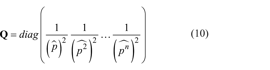
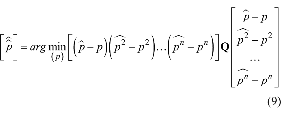
So the inversion procedure consists of two steps. First, we can use LSQ or NNLSQ technique to estimate vector $\hat{p}$ , then the crack depth can be estimated from all values of the vector $\hat{p}$ using WLSQ technique.

Crack depth estimation

Construction of polynomial direct model

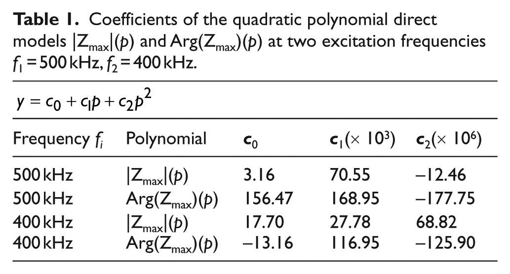
Starting from |Z_max| and Arg(Z_max) at two frequencies (f₁ = 500 kHz, f₂ = 400 kHz) we have constructed polynomial direct models of these quantities as a function of p, according to the method described in section “Model-based inversion.” These models concern tested samples of the first group. The coefficients of these polynomials whose degree has been chosen equal to 2 are given in Table 1. According to the literature,²⁷ polynomials of degree above 2 are rarely used for inverse problem. Moreover, with regard to our problem, we have only three measurement points corresponding to the three cycles of impact force. Therefore, the choice of polynomials of degree greater than 2 would strongly lead to an over-fitting of the direct model to the data and to be detrimental to the estimation of p.

Table 1.

Coefficients of the quadratic polynomial direct models |Z_max|(p) and Arg(Z_max)(p) at two excitation frequencies f₁ = 500 kHz, f₂ = 400 kHz.

$y = c_{0} + c_{1} p + c_{2} p^{2}$
Frequency f_i	Polynomial	c0	c1(× 103)	c2(× 106)
500 kHz	\|Z_max\|(p)	3.16	70.55	−12.46
500 kHz	Arg(Z_max)(p)	156.47	168.95	−177.75
400 kHz	\|Z_max\|(p)	17.70	27.78	68.82
400 kHz	Arg(Z_max)(p)	−13.16	116.95	−125.90

Implementation of the inversion

We have tested the inversion of the different combinations of four polynomial direct models (|Z_max| and Arg(Z_max) at two frequencies f₁ and f₂), either mono-frequency or bi-frequency. As presented in section “Model-based inversion,” we implement two inversion techniques, called the LSQ-WLSQ and the NNLSQ-WLSQ. Each one consists of two estimation steps. It means, for the first step, in the first and the second inversion technique, the LSQ and the NNLSQ criterion²⁸ are used to estimate the vector p , respectively. Then, in the second step of both techniques, the WLSQ is applied to estimate the crack depth p. To compare and select an appropriate technique, we should consider the quantity of mean square error (MSE). The root mean square error (RMSE) of the crack depth p at all n measuring points, received after three impact cycles of a tested structure, is defined as equation (11)

R M S E = \sqrt{\frac{1}{n} \sum_{i = 1}^{n} {({\hat{p}}_{i} - p)}^{2}}

(11)

where ${\hat{p}}_{i}$ , $p$ are the ith estimation result and the true value of the crack depth, at each measuring point, respectively.

The comparison of different combinations of features (Table 2) shows that the combination of |Z_max| at two excitation frequencies f₁ and f₂ gives the most accurate estimation results, that is, we have the lowest mean squared error. By this combination, the best estimation results are obtained on both LSQ-WLSQ and NNLSQ-WLSQ techniques. For these two inversion techniques, the second is slightly more accurate than the first. The difference on RMSE between two techniques is of 4%–16% depending on the combination of the considered features. The difference of 4% corresponds to the most interesting combination—the combination of |Z_max| at the two excitation frequencies. By the addition of a non-negativity constraint, it improves the accuracy of the estimation results. The NNLSQ criterion is considered to give better results than the LSQ criterion when facing with noisy data.

Table 2.

Comparison of the LSQ-WLSQ and NNLSQ-WLSQ inversion techniques, applied to different polynomial direct models to estimate the depth of cracks at f₁ = 500 kHz, f₂ = 400 kHz.

Used features	RMSE (µm)	1 – RMSE/RMSE_min
LSQ-WLSQ inversion
\|Z_max\| at f₁ and f₂	51.52 (RMSE_min)
\|Z_max\| and Arg(Z_max) at f₁ and f₂	68.13	24.4%
\|Z_max\| and Arg(Z_max) at f₁	91.95	44.0%
NNLSQ-WLSQ inversion
\|Z_max\| at f₁ and f₂	49.38 (RMSE_min)
\|Z_max\| and Arg(Z_max) at f₁ and f₂	57.11	13.5%
\|Z_max\| and Arg(Z_max) at f₁	87.22	43.4%

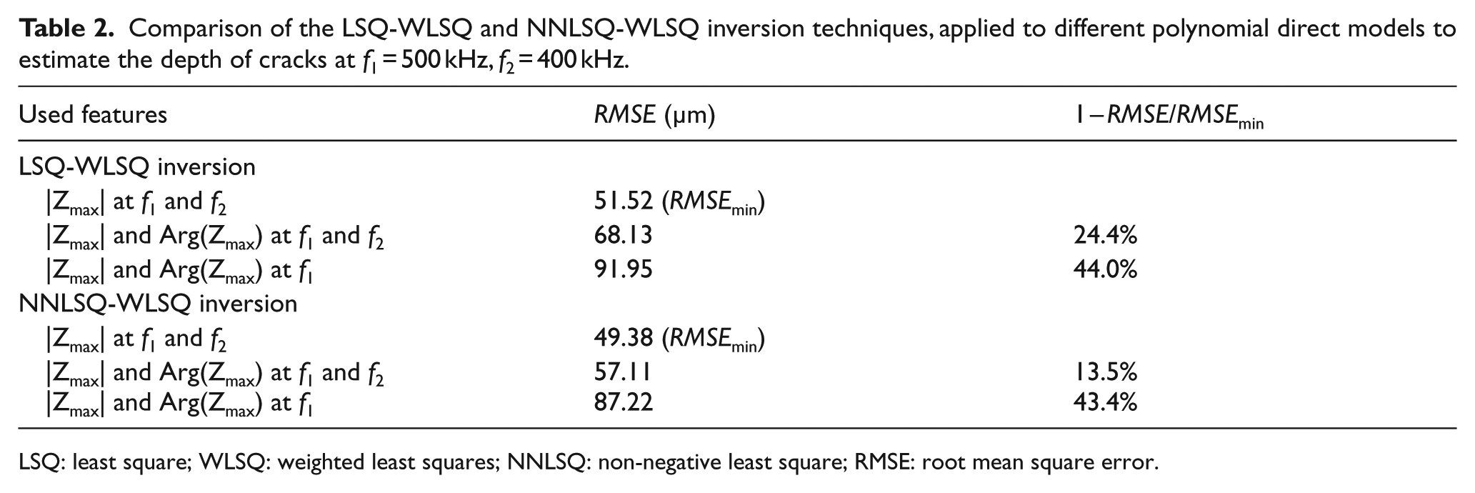
LSQ: least square; WLSQ: weighted least squares; NNLSQ: non-negative least square; RMSE: root mean square error.

In the case of the inversion using bi-frequency polynomial models of |Z_max|, knowing that the crack depths to be estimated are between 200 and 800 μm, from the RMSE is about 50 μm, we can say that the proposed estimation method is satisfactory. These accurate estimations can be verified graphically in Figure 11, where the estimation results are obtained from two tested samples M11 and M12 and using NNLSQ-WLSQ technique.

Figure 11.

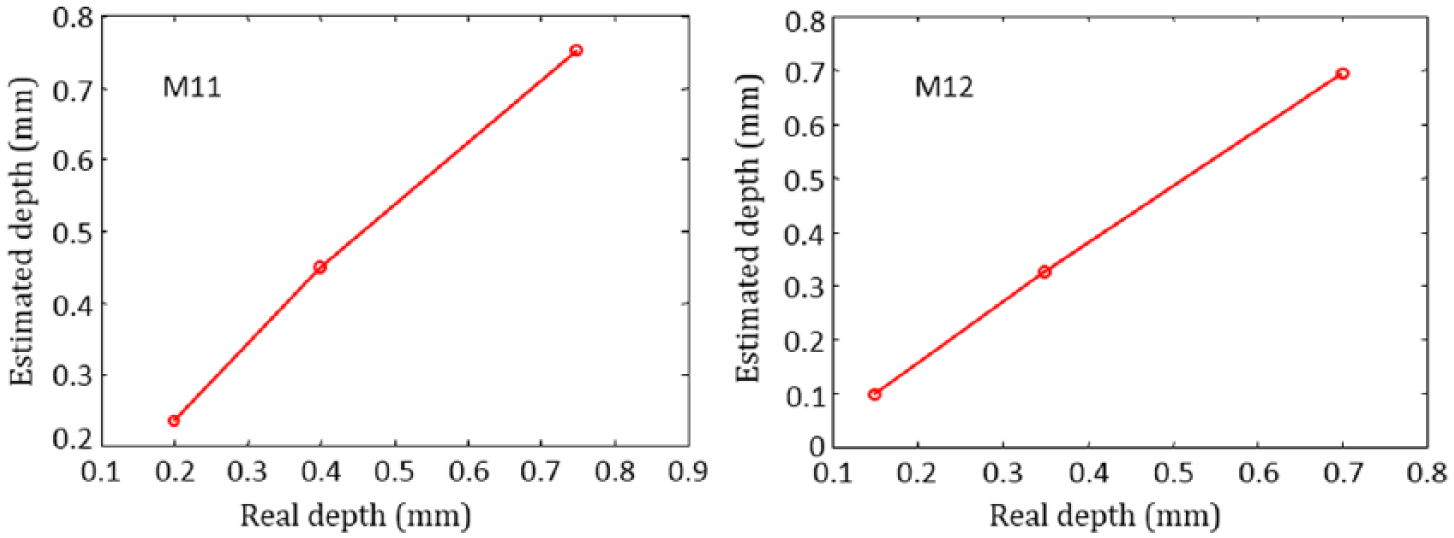
The obtained estimation results on tested samples M11 and M12 using the NNLSQ-WLSQ inversion technique with the bi-frequency polynomial direct model (400 and 500 kHz) of |Z_max|.

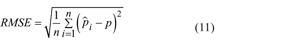
Moreover, the precision of estimation results is also analyzed through the relative error—RE, defined as in equation (12)

R E % = \frac{\hat{p} - p}{p} \cdot 100

(12)

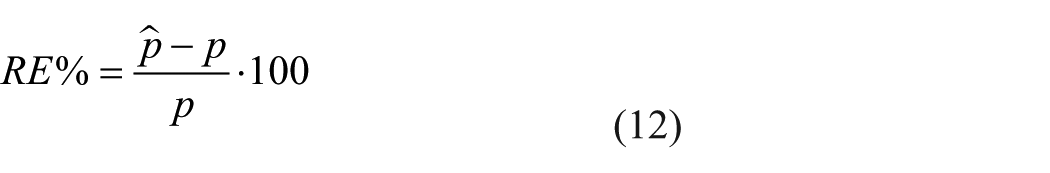
where $\hat{p}$ and p are the estimated and true value of crack depth p, respectively.

As shown in Table 3, based on the relative error, it is generally observed that the greater the crack depth, the more precise the estimation. But some values of RE in Table 3 do not match with this trend. The reason is that the database used to construct the direct model is limited, so when a crack depth is far from the general trend, given by a group of tested samples, the estimation is not precise. With the most favorable polynomial model, the estimation results are satisfied for the depth of crack at the end of the third cycle (being largest, between 0.7 and 0.75 mm). Indeed, in this case, the maximum bias is –4.8% (Table 3). However, the bias of the estimation is higher for shallower depths, and the precision in some cases is insufficient (RE = 58.63% for the model M13 after the first cycle, RE = –26.53% for the model M14 after the second cycle).

Table 3.

Crack depth estimation by bi-frequency method, based on the inversion of polynomial direct model using NNLSQ-WLSQ technique.

RE (%) (bi-frequency polynomial model (400 and 500 kHz) of \|Z_max\|)
Tested sample	M11	M12	M13	M14
First cycle	17.45	−34.53	58.63	3.88
Second cycle	12.20	−7.32	−16.84	−26.53
Third cycle	0.27	−1.01	1.69	−4.80

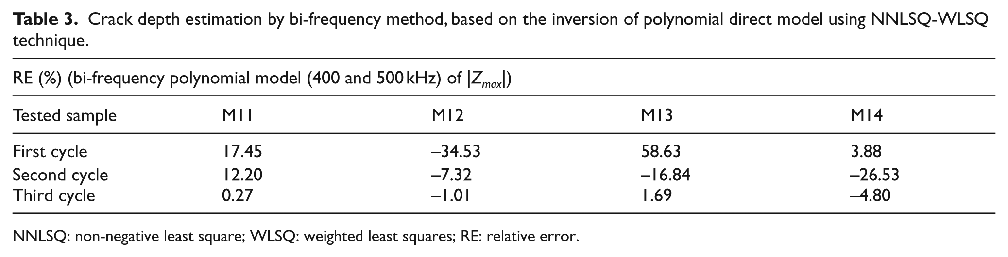
NNLSQ: non-negative least square; WLSQ: weighted least squares; RE: relative error.

Conclusion

In this paper, we proposed an approach to estimate the crack depth on a massive plate. The approach is constructed based on the analysis of EC images of real sub-millimeter cracks on a limited set of tested samples. The model-based approach proposed in this study is easy to implement.

Among the proposed models, the estimation method based on a bi-frequency quadratic polynomial model of |Z_max| is the one that gives the best results. The obtained estimation results have an acceptable precision (Table 3), and the RMSE is about 50 μm for crack depths in the range between 200 and 800 μm (Table 2). While these results are promising, it would appear that a wider database would be useful for constructing more accurate direct models and thereby improving the estimation results in terms of reducing their bias and variance.

Footnotes

Declaration of conflicting interests

The author(s) declared no potential conflicts of interest with respect to the research, authorship, and/or publication of this article.

Funding

This research was funded by Vietnam National Foundation for Science and Technology Development (NAFOSTED) under grant number 103.99-2014.31.

References

Kermadi

Moussaoui

Brahimi

et al . Defect localization and characterization in Eddy current nondestructive testing by change detection and global optimization. COMPEL 2017; 37: 948–970.

Cheng

Qiu

et al . Research advances in eddy current testing for maintenance of carbon fiber reinforced plastic composites. Int J Appl Electrom 2016; 51: 261–284.

Zeng

Huang

et al . Frequency-domain defect characterization in pulsed eddy current testing. Int J Appl Electrom 2014; 45: 621–625.

Xie

Chen

H-E

et al . Evaluation of plastic deformation and characterization of electromagnetic properties using pulsed eddy current testing method. Int J Appl Electrom 2014; 45: 755–761.

Vernon

SN.

The universal impedance diagram of the ferrite pot core eddy current transducer. IEEE T Magn 1989; 25: 2639–2645.

Janousek

Stubendekova

Smetana

Novel insight into swept frequency eddy-current non-destructive evaluation of material defects. Measurement 2018; 116: 246–250.

Cung

Joubert

Vourch

Eddy current evaluation of air–gaps in aeronautical multilayered assemblies using a multi-frequency behavioral model. Measurement 2011; 44: 1108–1116.

Chen

Tian

Sophian

et al . Feature extraction and selection for defect classification of pulsed eddy current NDT. NDT&E Int 2008; 41: 467–476.

Edwards

Sophian

Dixon

et al . Dual EMAT and PEC non-contact probe: applications to defect testing. NDT&E Int 2006; 39: 45–52.

10.

Tian

Sophian

Defect classification using a new feature for pulsed eddy current sensors. NDT&E Int 2005; 38: 77–82.

11.

Weekes

Almond

Cawley

et al . Eddy-current induced thermography—probability of detection study of small fatigue cracks in steel, titanium and nickel-based superalloy. NDT&E Int 2012; 49: 47–56.

12.

Deng

Kang

Zhang

et al . Multi-source effect in magnetizing-based eddy current testing sensor for surface crack in ferromagnetic materials. Sensor Actuat A: Phys 2018; 271: 24–36.

13.

Zhou

Wang

et al . Influence of metallic shields on pulsed eddy current sensor for ferromagnetic materials defect detection. Sensor Actuat A: Phys 2016; 248: 162–172.

14.

Horan

Underhill

Krause

TW.

Pulsed eddy current detection of cracks in F/A-18 inner wing spar without wing skin removal using Modified Principal Component Analysis. NDT&E Int 2013; 55: 21–27.

15.

Yang

Tamburrino

Udpa

et al . Pulsed eddy-current based giant magnetoresistive system for the inspection of aircraft structures. IEEE T Magn 2010; 46: 910–917.

16.

Cheng

Tian

GY.

Surface crack detection for carbon fiber reinforced plastic (CFRP) materials using pulsed eddy current thermography. IEEE Sens J 2011; 11: 3261–3268.

17.

Tian

Pan

et al . Impact evaluation in carbon fiber reinforced plastic (CFRP) laminates using eddy current pulsed thermography. Compos Struct 2014; 109: 1–7.

18.

Gao

Woo

et al . Quantitative surface crack evaluation based on eddy current pulsed thermography. IEEE Sens J 2017; 17: 412–421.

19.

Granville

Charlton

Detection and sizing of baffle plate erosion and fretting using eddy current array technology, http://repository.uwtsd.ac.uk/679/ (2016, accessed 9 May 2017).

20.

Yuan

Spiessberger

Waag

TI.

Eddy current thermography imaging for condition-based maintenance of overlay welded components under multi-degradation. Mar Struct 2017; 53: 136–147.

21.

Zhou

Xie

et al . Investigation on eddy current pulsed thermography to detect hidden cracks on corroded metal surface. NDT&E Int 2016; 84: 27–35.

22.

Gao

Tian

et al . Multiple cracks detection and visualization using magnetic flux leakage and eddy current pulsed thermography. Sensor Actuat A: Phys 2015; 234: 269–281.

23.

Cheng

Kanemoto

Komura

et al . Depth sizing of partial-contact stress corrosion cracks from ECT signals. NDT&E Int 2006; 39: 374–383.

24.

Ravat

Conception de multicapteurs à courants de Foucault et inversion des signaux associés pour le contrôle non destructif. PhD Thesis, Université Paris Sud-Paris, 2008, https://tel.archives-ouvertes.fr/tel-01022823/document

25.

Yusa

Hashizume

Urayama

et al . An arrayed uniform eddy current probe design for crack monitoring and sizing of surface breaking cracks with the aid of a computational inversion technique. NDT&E Int 2014; 61: 29–34.

26.

Courrieu

Fast solving of weighted pairing least-squares systems. J Comput Appl Math 2009; 231: 39–48.

27.

Dood

Deeds

Analytical solutions to eddy-current probe-coil problems. J Appl Phys 1968; 39: 2829–2838.

28.

Lawson

Hanson

. Solving least squares problems. SIAM, Philadelphia, PA 19104-2688 USA, 1995.

A model-based approach for estimation of the crack depth on a massive metal structure

Abstract

Keywords

Introduction

Problem formulation

Processing and feature extraction of sensor impedance images

Reduction of the influence of noise existing at the edges of images

Subtraction of the complex image background

Analysis and identification of interesting magnitudes in EC images

Estimation of |Zmax| and arg(Zmax)

Behavioral study: evolution of |Zmax| and Arg(Zmax) as a function of p

Model-based inversion

Polynomial direct model

LSQ and weighted least squares inversion procedure

Crack depth estimation

Construction of polynomial direct model

Implementation of the inversion

Conclusion

Footnotes

Declaration of conflicting interests

Funding

References

Estimation of |Z_max| and arg(Z_max)

Behavioral study: evolution of |Z_max| and Arg(Z_max) as a function of p