
Abstract
This paper presents the adaptive model predictive control approach for a two-wheeled robot manipulator with varying mass. The mass variation corresponds to the robot picking and placing objects or loads from one place to another. A linear parameter varying model of the system is derived consisting of local linear models of the system at different values of the varying parameter. An adaptive model predictive control controller is designed to control the fast-varying center of gravity angle in the inner loop. The reference for the inner loop is generated by a slower outer loop controlling the linear position using a linear quadratic Gaussian regulator. This adaptive model predictive control/linear quadratic Gaussian control system is simulated on the nonlinear model of the robot, and the closed-loop performance of the proposed scheme is compared with a system having inner/outer loop controllers as proportional integral derivative/proportional integral derivative, feedback linearization/linear quadratic Gaussian, and linear quadratic Gaussian/linear quadratic Gaussian. It is seen that adaptive model predictive control shows mostly superior and otherwise very good performance when compared to these benchmarks in terms of reference tracking and robustness to mass parameter variations.
I. Introduction
Mobile robot applications are growing in significance in research and daily-life implementations. These robots are commonly used in a wide range of fields and applications such as in industrial plants, commercial zones, medical systems, material handling, and the defense industry. The major advantage and superiority of mobile robots over legged counterparts are design and control simplicity, reduced manufacturing and maintenance costs, and longevity. The legged-robots are also capable of tackling obstacles and uneven terrain difficulties. 1 However, it is a tedious task to maintain the control of a legged-robot due to the complexity of its structure. 2 Mobile robots can be mainly configured as three-, four-, and six-wheel structures, which are statically stable systems for ease of control and energy efficiency. Among these the most popular one is the four-wheel structure, ensuring stability at high speeds and under certain disturbances. On the other hand, due to the physical characteristics of four wheels, it is dependent on suspension systems to keep the wheels in contact with the road.
Besides these configurations, there are also two-wheeled mobile robots available. Two-wheeled mobile robots are basically called “two-wheeled balancing robots” (TWBR) due to their unstable dynamical characteristics. Although controlling two-wheeled robots is a challenging issue, they can be regarded as simpler structured mechanisms than legged-robots. Their advantages over other configurations are high maneuverability capabilities, small footprints, and ability to turn around their own axis, but they can be less power efficient due to the continuous need to balance. However, thanks to this continuous dynamical stabilization, the robot can reject disturbances affecting the body and can have a wider range of center of gravity (COG) variance. This lets the designer place additional payloads and structures on the system. 3 The most common structure of the TWBR is two electrical-motor-powered wheels connected to the main stationary body. The stationary part of the robot is essentially an inverted pendulum whose stability must be achieved with the effort of the two actuated wheels. 4
Due to structural advantages and being a challenging control problem, TWBR is an important problem attracting interest in numerous research and application works.4,5–9 Linear controllers such as proportional integral derivative (PID) and linear quadratic Gaussian (LQR) can be designed and comprehended easier than complex nonlinear and adaptive ones.
10
For this purpose, a linear dynamical model of the system is derived around predefined equilibrium points. For a given linearized model, it is straightforward to apply established methods such as pole placement
11
and LQR12,13 to maintain the stability of the system. Various studies also show comparisons among different linear control schemes.14,15 The performance of the linear controllers is dependent on the selection of the control parameters such as
Despite the availability of advanced methods, simple PID designs still dominate industrial applications due to their simple structure and ease of tuning.20,21 Since PID controllers are essentially single-input single-output in nature, multiple controllers must be designed for the tilt angle and position of the vehicle. 22 These two modes must also be assumed to be decoupled, which may prove to be incorrect if the departure from the operating point is large. Employing nonlinear control techniques could remedy this drawback allowing the designer to work on a wider scale of operating conditions.23,24 For instance, the combination of PID and backstepping controllers are presented and the advantages of each method are depicted in Lee et al. 25 Sliding mode control (SMC) is also possible, a method known for its powerful capabilities and robustness against system uncertainties and perturbations. 26 SMC drives the system to a predefined hypersurface and ensures exponential convergence to origin, while rejecting disturbances and perturbations. 27 Another possibility is feedback linearization (FBL; i.e. dynamic inversion), where the system nonlinearities are cancelled through feedback, after which the problem reduces to linear control.28,29 Numerous other nonlinear control approaches were tested on TWBR systems, including fuzzy PID with satisfactory results. 30
Adaptive control strategies are methods applicable to time-varying and uncertain systems for maintaining performance criteria and stability. Myriad studies are available varying from simple double integrator systems to complex chemical processes. 31 Different adaptive control strategies were successfully implemented on TWBR as well. In Degani et al., 32 the center of mass height was tracked by checking the deviation from the COG and the system was kept stable with adaptive control techniques. Adaptive and fuzzy controllers were merged for real-time adjustment of the membership functions in Wang et al. 33 Other examples include neural-adaptive output feedback control of transportation vehicles based on wheeled inverted pendulum models 34 and two-timescale-tracking control of nonholonomic wheeled mobile robots. 35
Model predictive control (MPC) strategy is widely used in the process control industry, especially for systems with slow dynamics. The MPC performance depends on the dynamical model of the process or system. MPC takes the current time into account, sustaining optimality while keeping incoming future timeslots. This is an iterative and finite time horizon optimization method. MPC achieves prediction of the future states of the linear time-invariant (LTI) model of the nonlinear plant linearized around specific equilibrium points. Practically, the prediction of MPC is sensitive to prediction errors. This is acceptable for lowly nonlinear systems. On the other hand, TWBR includes highly coupled nonlinear dynamics, limiting the ability of MPC control to achieve satisfactory performance and stability. To resolve this problem, adaptive model predictive control (AMPC) can be employed. 36 AMPC can handle performance degradation of the MPC controller due to the strong nonlinearity. AMPC uses changing operating points to update the prediction model. The advantage of using AMPC is the convenience of constructing on a predesigned MPC structure. Studies on the AMPC control scheme applied to different systems are becoming more appealing as computing capabilities increase.37,38
In this study, we investigate combining a TWBR base with a robot manipulator, in particular controlling its position. This generates a type of robotic system valuable for industrial and daily-life applications. A robot manipulator consists of one or more rigid links connected via fixed or actuated joints. Robot manipulators are useful for picking/placing objects, assembly, and applications hazardous/inappropriate for humans. Their disadvantage is limited workspace due to a fixed base point. Integrating with a TWBR could thus remedy this drawback, achieving high mobility and maneuverability in diverse environments.39,40 The benefits of such integration are summarized in Figure 1 . The aim of this study is to prove the usefulness of AMPC for such an integrated robot, in the sense that desired tracking performance outperforms various standard control approaches. Our method builds upon a new linear parameter varying (LPV) modeling approach,41–45 so that mass variations corresponding to the robot manipulator’s actions are captured. Typical robot manipulators are actuated systems since the number of degrees of freedom and actuators are equal. After merging a TWBR with a robot manipulator the system becomes underactuated, and from the controller’s perspective it is similar to an inverted pendulum on a cart. 46 In this study the setup investigated consists of four manipulator links, which are considered as one virtual link. The use of this equivalence allows simpler dynamical modeling. The control goal is to robustly track position while coping with this underactuated structure, nonlinear dynamics, and disturbances from various sources.
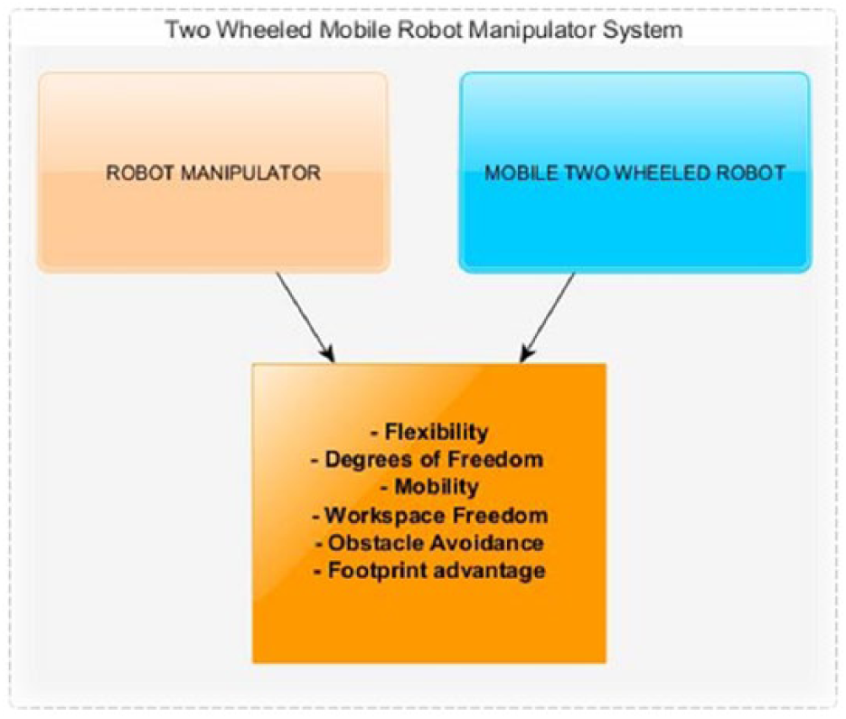
Mobile robot system.
The rest of this paper is organized as follows: Mathematical modeling of system is presented first, deriving the equivalent inverted pendulum representation. Once the model is obtained, various control approaches are developed, consisting of an inner loop for the faster angle dynamics, and an outer loop for the slower linear position. These approaches considered are PID/PID, LQG/LQG, FBL/LQG, and finally AMPC/LQG, where the X/Y notation denotes X for inner controller and Y for outer controller. Simulations are carried out for all, where a reference trajectory is tracked in the presence of mass variations. The results are evaluated in terms of various metrics. The paper ends with conclusions and future directions.
II. Mathematical Modeling
In order to design and implement controllers, an appropriate model of the proposed system was created under MATLAB/Simulink numerical computing environment. During the modeling phase, different toolboxes were employed such as SimMechanics and control systems. The system configuration is based on the study of Chen et al., 39 which is illustrated in Figure 2 . The manipulator consists of four links as seen in the figure. The first link, that is, the link connected to the wheel, is passive while the others are actuated.
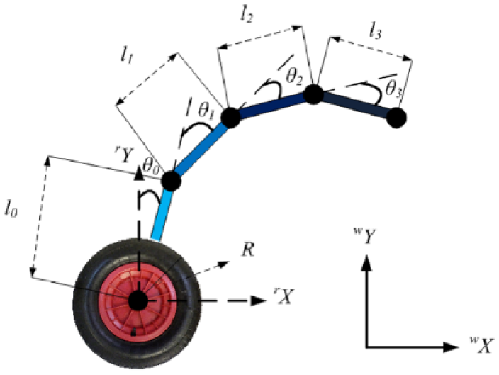
Mobile manipulator model.
The parameters of the robot are as follows:
The governing equations describing the motion of the mobile robot manipulator are

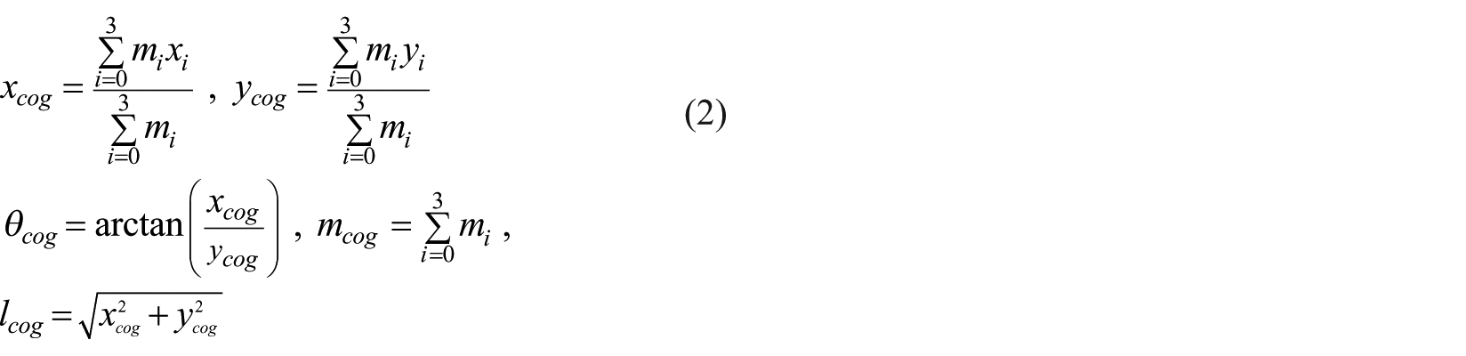
where τ = [τw, 0, τ1, τ2, τ3] is the input torque, θ = [θw, θ0, θ1, θ2, θ3] is the vector of angles, and M, H, q(θ) are, respectively, the inertia, centrifugal force, Coriolis force, and gravity matrices. Due to the complex structure of the robot manipulator, system modeling requires many equations to describe the entire system. Having four links is useful in terms of extended physical capabilities, but increases model complexity. In order to simplify modeling, the system could be considered as a single rod virtual inverted pendulum as shown in Figure 3 . As depicted in the model, mass and inclination of four links are represented by a virtual link mass at the COG and its angle with the wheel. These can be computed with the following mathematical calculations
At this point Euler-Lagrange method can be employed for derivation of the dynamical model of the inverted pendulum. The dynamical equation of motion of entire system can be written as follows

where
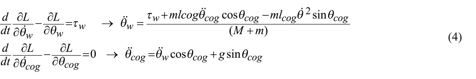
where M is the mass of the mobile part and m is the mass of COG, respectively.
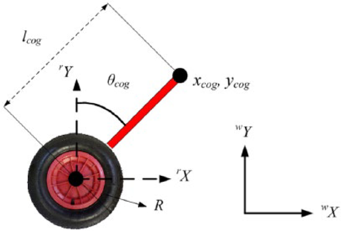
Virtual inverted pendulum model.
An important aspect of this research is to have a variable mass on the robot to carry out various tasks. While handling different tasks, the system acts like a time-variant system as the mass of entire body changes at the time frame of working, for instance, when the robot picks a load from a point and drops off in a different location. If the system is not designed with robustness enough to handle the effect of mass variance, stability and reference tracking may not be sustained, causing violent oscillations or instability. To compare the difference, the robot is modeled under two conditions, namely, with variance in mass and without variance in mass. Pick and place scenarios were applied in the simulation studies. Figure 4 shows the three-dimensional (3D) model of the manipulator realized in SimMechanics.
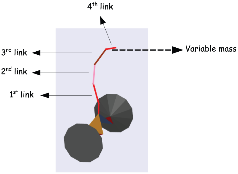
Variable mass scenario.
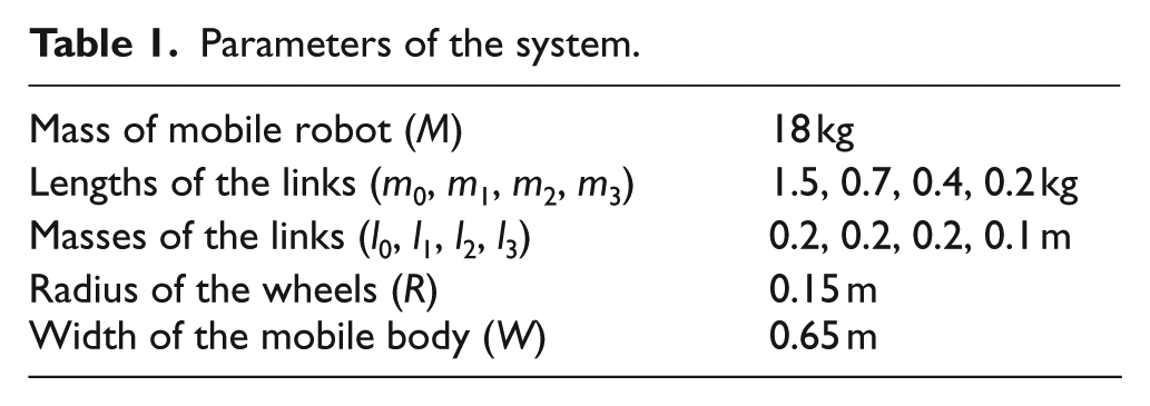
The Simulink block diagram is given in Figure 5 and the key parameters of the system are depicted in Table 1 . In the block diagram, the joint between the first link and the main body is unactuated while the other joints are actuated by the controller. Unlike the other links, the last link was modeled adding variable a mass input to the arm representing picking up or putting down objects. This mass variance effect is a key consideration in mathematical modeling and controller design.
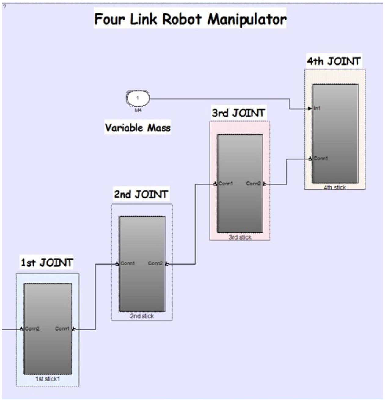
Robot manipulator modeling via SimMechanics.
Parameters of the system.
III. Control Design
Due to its statically unstable structure, a dynamic controller is required to maintain stability of the balancing robot. The ultimate objective in control is balancing the COG of the virtual link, whose position, angle, and mass will change based on the task carried out by the manipulator. Thus, a robust control system to suppress the adverse effects of the disturbances, perturbations, unmeasured dynamics, and variable mass is needed to handle the control task. The robot system is underactuated from the perspective of controlling the COG; only the wheels provide the control (see Figure 5 ). There are, however, 2 degrees of freedom, namely, the location of the COG and the linear position of the robot, which have coupled dynamics between each other. The challenge is therefore to control a coupled dynamics with only one input.
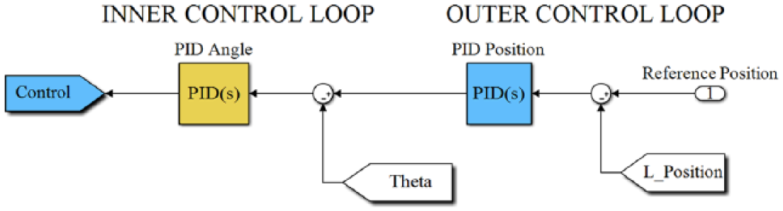
The control systems literature offers a wide range of solutions when it comes to controlling underactuated dynamical systems. The dynamics of the mobile robot manipulator are such that the 2 degrees of freedom can be categorized as fast and slow dynamics. The fast dynamics are those related to the inner loop of the vehicle, that is, the angle of the link. The slow dynamics are those related to the outer loop of the vehicle, that is, the linear position of the wheels. In control design the major emphasis is placed on stabilization of fast dynamics, which plays a significant role in the behavior of the vehicle as a whole. The slow dynamics, that is, linear position, is then controlled as an outer loop by manipulating the angle inside the inner loop ( Figure 6 ). Various control design methods are implemented in the succeeding sections and are compared in terms of the metrics integral absolute error (IAE), mean absolute error (MAE), integral squared error (ISE), and integral squared control input (ISCI).
Closed-loop structure of the proposed system.
IV. Proportional Integral Derivative Control Scheme
PID control is one of the earliest yet most popular control schemes due to the ability to perform easy empirical tuning for satisfactory performance. 40 To design the PID controller, nonlinear dynamics of the vehicle are first linearized around the zero equilibrium point (i.e. when the robot is stationary in an upright position). Then dynamics of rotational behavior (COG angle) are control by tuning the coefficients of the inner PID controller until satisfactory performance. Next, for controlling the linear position the coefficients of the outer loop PID are adjusted, fixing the inner PID controller. The process is iterated a number of times until the angle and position responses are as desired. Further fine-tuning is performed to account for the effects caused by mass variations. The ultimate values of the inner loop coefficients are Kp1 = −77.306, Ki1 = −8.721, and Kd1 = −28.862 and those of the outer loop are Kp2 = 0.426, Ki2 = 0.02, and Kd2 = 1.319. It is expected that larger control coefficients are required for the inner loop PID controller because tracking and stabilizing of the fast dynamics need more aggressive control effort. The block diagram implementation of the control system can be seen in Figure 7 . For realistic simulations, measurement noise is also added to the angle and position inputs of the control.
Cascaded PID control structure.
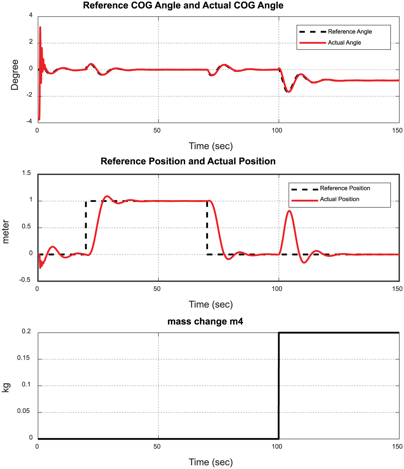
The results of the PID control approach can be observed in Figures 8 – 10 . According to the simulation scenario, mass of the last link, that is, link 4, is changed from 0.2 to 0.4 kg at t = 100 s in order to test the robustness of the controlled plant against variances in mass. The initial conditions for the links are, respectively, −10, 10, 10, and 10°. The angular control loop exhibits sufficient performance and the position controller shows good tracking performance until 100 s. With the change of mass of the last link at time t = 100 s, the position controller performance severely deteriorates and takes a significant time to settle. The performance metrics for the PID controller are tabulated in Table 2 .
PID angular and positional tracking with mass change at 100 s.
Transient and parameter change responses.
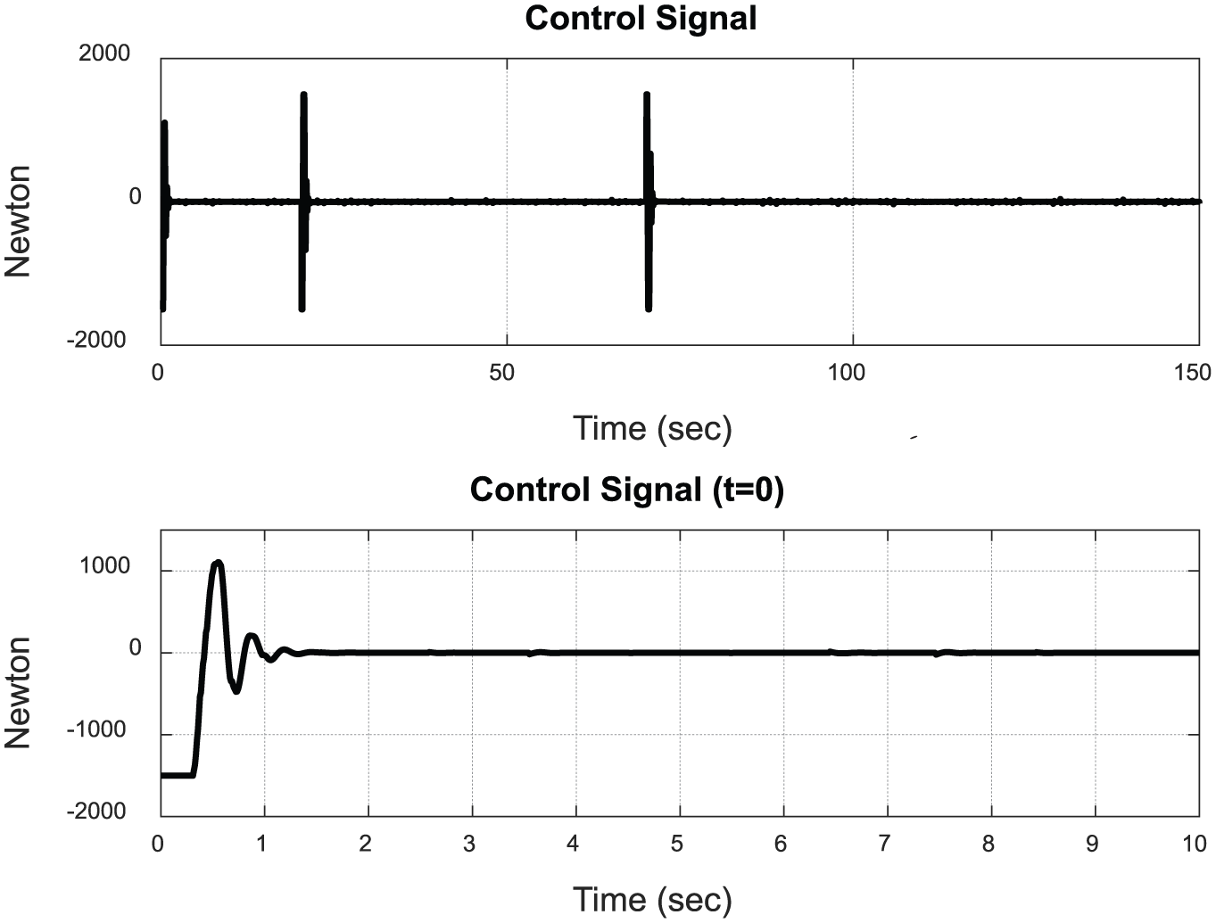
Control signal under PID control.
Performance measures for PID control scheme.
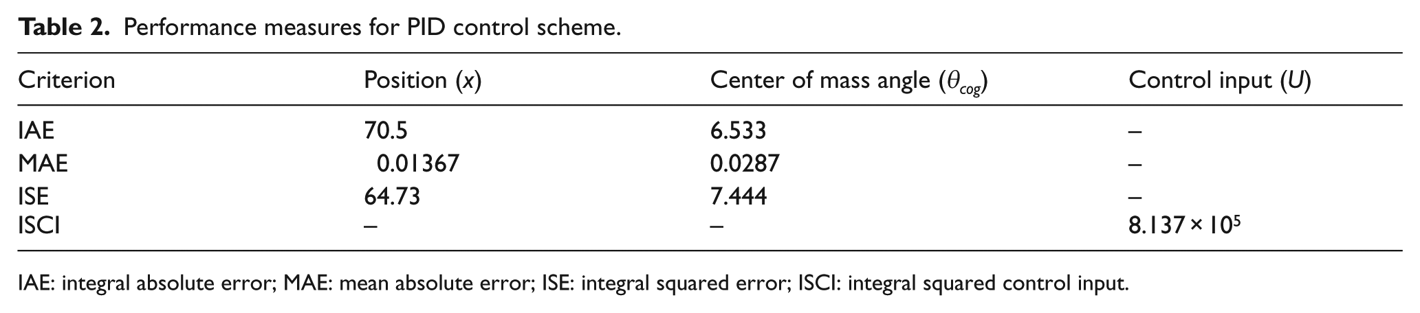
IAE: integral absolute error; MAE: mean absolute error; ISE: integral squared error; ISCI: integral squared control input.
V. Linear Quadratic Gaussian Control
LQG is a dynamical controller for the system written in the form

where x is state vector, u is plant input, y is the plant output, w is the process noise representing modeling errors, and v is the output noise representing measurement errors. A, B, C, D are the state-space matrices. LQG is in fact a combination of the linear quadratic regulator (LQR), an optimal controller, and the Kalman filter, an optimal estimator. The objective of the LQR controller is to minimize the cost function J

where E denotes the expected value, xi is integral of the reference tracking error of the output signal, and Q, R, Qi are, respectively, weighing matrices for states, input, and integral error. Due to the lack of measurements from all states of the system, a Kalman filter is employed which provides optimal estimates for x (denoted xe) by minimizing the function

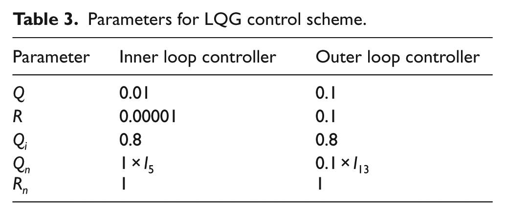
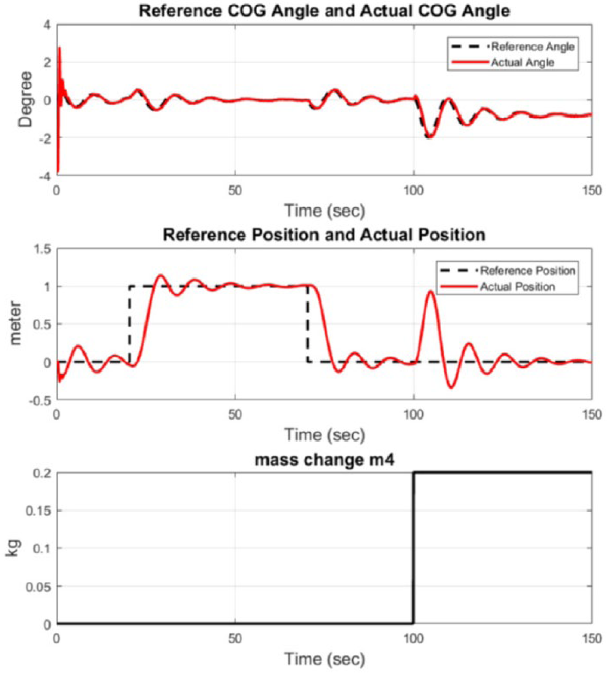
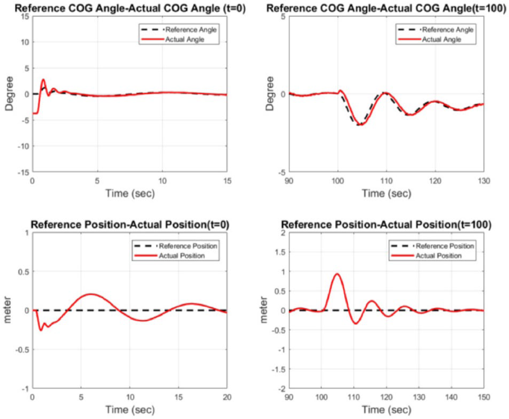
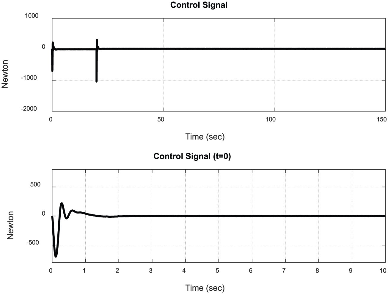
given the process and measurement noise covariances Qn and Rn. During the design phase of the LQG controller, the system is again linearized around the zero equilibrium point and the design is carried out by selecting the parameters as in Table 3 . The results for the LQG controller system can be seen in Figures 11 – 13 . The figures correspond to the COG angle, linear position tracking, variable mass change, and control effort, respectively. It can be observed from the figures that both the LQG controllers are capable of following and suppressing the effect of the changing mass at t = 100 s. After some fluctuation the system settles down to steady state within about 20 s. The performance metrics for LQG are shown in Table 4 . It is seen that the ISCI index is lower than PID, that is, less control effort is required. All the error metrics (IAE, MAE, ISE) are also lower, meaning that the LQG controller has better reference tracking and robustness to parameter variations.
Parameters for LQG control scheme.
LQG angular and positional tracking with mass change.
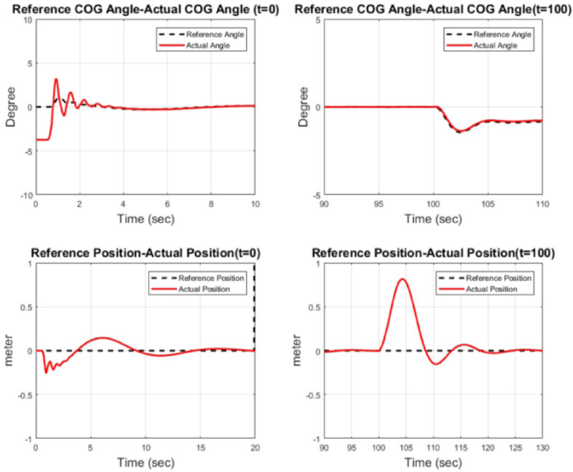
Transient and parameter change responses.
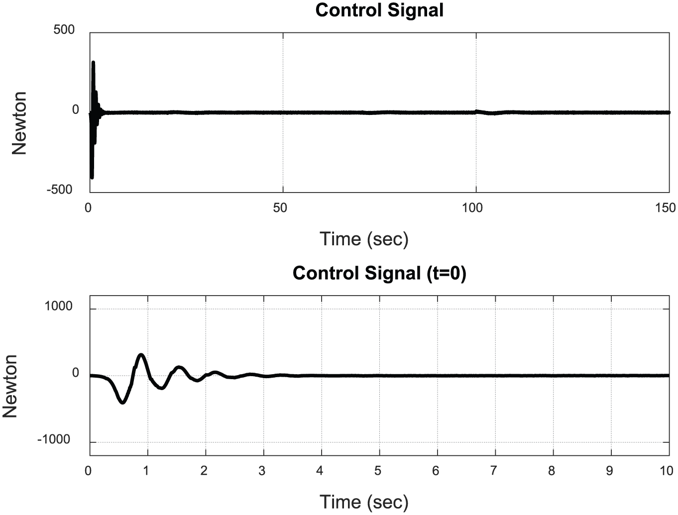
Control signal of LQG.
Performance measures for LQG control scheme.
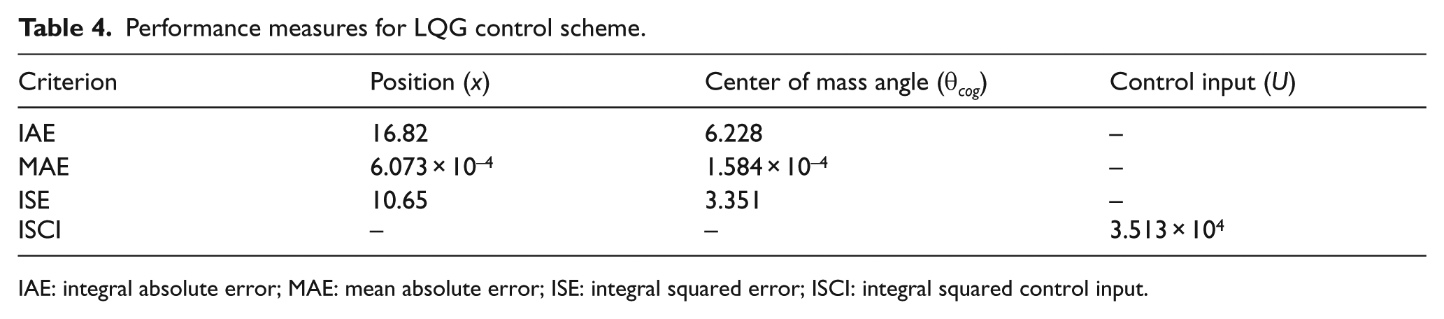
IAE: integral absolute error; MAE: mean absolute error; ISE: integral squared error; ISCI: integral squared control input.
VI. Feedback Linearization Control
FBL (also called dynamic inversion) is a nonlinear control approach that can produce exact linear representation of the plant model. FBL employs transformation of the nonlinear system into equivalent linear system by applying appropriate control input (Kim et al., 2010). 47 Since no approximation is made (in contrast to approximate Jacobian linearization), FBL is valid over the entire operating envelope and not just within a local neighborhood.
Let the dynamics of a nonlinear system be expressed as

where

so as to make the system exactly linear as

after which

where u is input torque to the wheels. This can be arranged as

which is of the form of equation (8). Utilizing an FBL controller of the form of equation (9)

yields

Let

where

which is asymptotically stable for

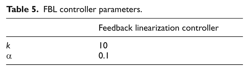
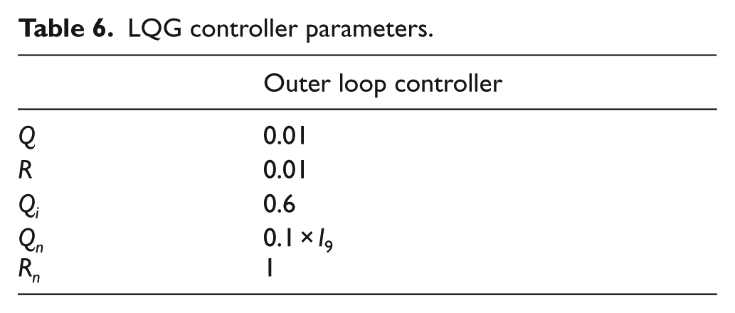
which completes the inner loop controller design via FBL. For the outer loop we utilize LQG to control the position, making this an FLB/LQG controller overall. After numerous iterations the controller parameters giving the best results are given in Tables 5 and 6. The simulation results with these parameters are plotted in Figures 14 – 16 . The controller starts out acceptably, albeit with some oscillations. The mass change at t = 100 s, however, degrades tracking considerably, which takes quite a while to settle back. The performance metrics are given in Table 7 . It is seen that the tracking performance is quite inferior to LQG. The control effort is somewhat lower, but this is of little value in presence of the degraded performance. Also, no clear advantage is obtained over PID as some metrics are higher, while some are lower.
FBL controller parameters.
LQG controller parameters.
FBL angular and LQG positional tracking with mass change.
Transient and parameter change responses.
Control signal of FBL.
Performance measures for FBL and LQG control schemes.
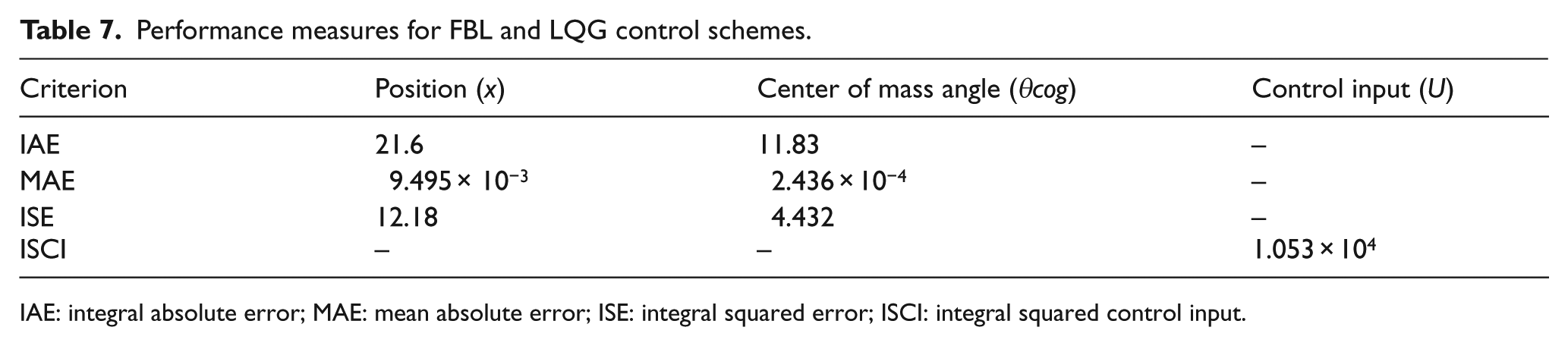
IAE: integral absolute error; MAE: mean absolute error; ISE: integral squared error; ISCI: integral squared control input.
VII. Adaptive MPC Control
Model predictive control (MPC) is a method for process control that actively uses the dynamical model of the system. The system is optimized within a predefined time slot in which MPC estimates the future states and controls of system. While this is quite computationally intensive, advances in digital computing have increased the feasibility of the MPC approach greatly. MPC can be implemented in the presence of uncertainties on linear and nonlinear systems. If the nonlinearity is high, however, MPC performance could deteriorate. In this case, one can use an adaptive model predictive controller that constantly predicts the new operating conditions. For instance, AMPC can be used on linear time-varying (LPV) systems with uncertainties, where the controller parameters are tuned in closed loop employing real-time measurements.41,46
The MPC algorithm solves a quadratic optimization problem at each time interval. The solution of the problem determines the so-called manipulated variables (MV), which are essentially the input variables adjusted dynamically to keep the controlled variables (CV) at their set-points. The AMPC approach follows the same cost optimization algorithm as MPC with the cost function
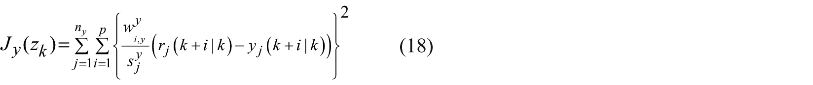
where k represents the current control interval, p is the prediction horizon (interval number), ny is the number of plant output variables, zk is the quadratic problem (QP) selection which is depicted as

where vk is the measurement noise and wk = [dk, ek] is the process noise. The future trajectories of the dynamical model are predicted over the prediction horizon Hp. Setting all wk = 0 for all prediction instances the equation becomes
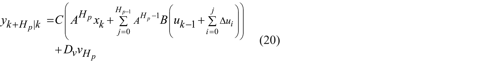
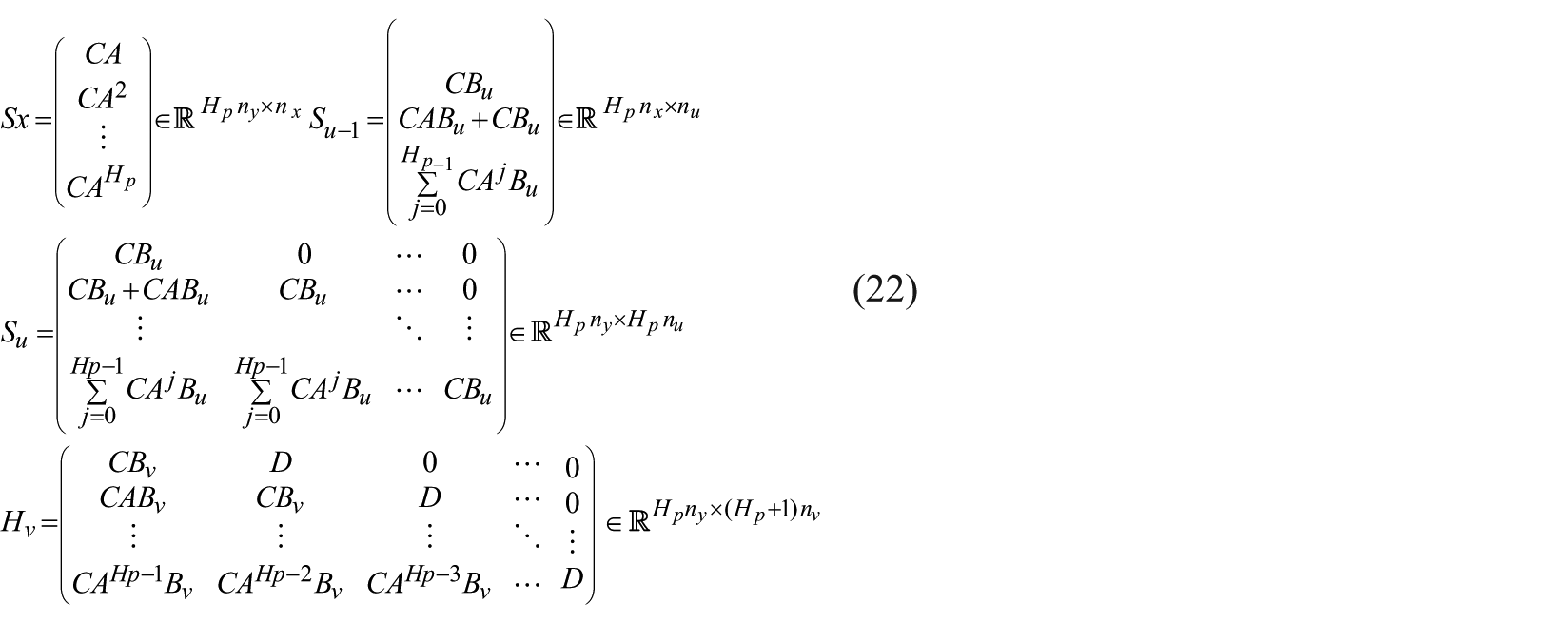
The solution can be summarized for all the Hp predicted time intervals as follows
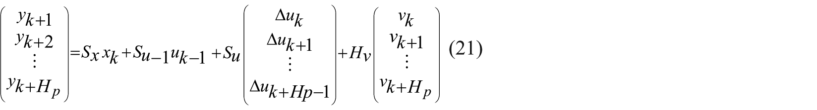
where
Regarding the equations mentioned above, the optimization function can be introduced as
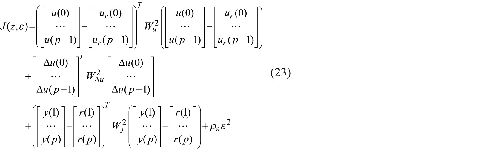
For the optimization function, the design parameters are the Wu, WΔu, and Wy matrices. Designing the MPC controller requires consideration of the constraints depicted as follows
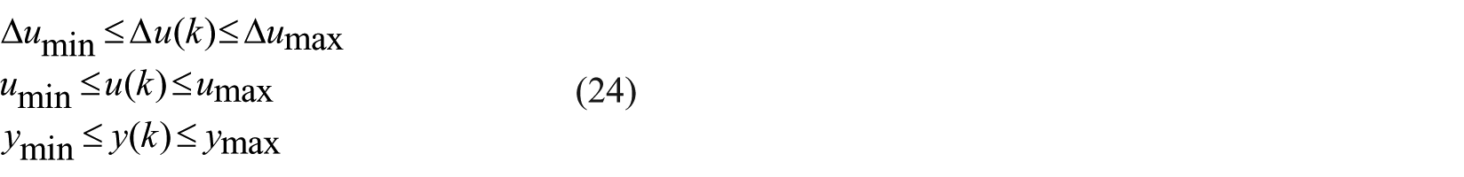
The constraints are on the inputs, input increments, and output variables with the slack variable ε ≥ 0. The parameter ρε is employed to penalize the constraint violation described before designing the controller. The optimization problem converted to a general QP is

obeying the condition of Ax ≤ b. Here xT =[zTε] is the decision vector, H is the Hessian matrix, A is the linear transition matrix, b and f are column vectors. The MPC controller uses the steady-state Kalman filter algorithm to estimate the state of the controller. In static Kalman filter (SKF), the L and M gain matrices are constant and they depend on the plant parameters, disturbances, and noise characteristics. In AMPC control, the controller uses the time-varying Kalman filter (TVKF) instead of the static one to provide consistent estimation with the updated plant dynamics. 20 The TVKF approach can be expressed as follows
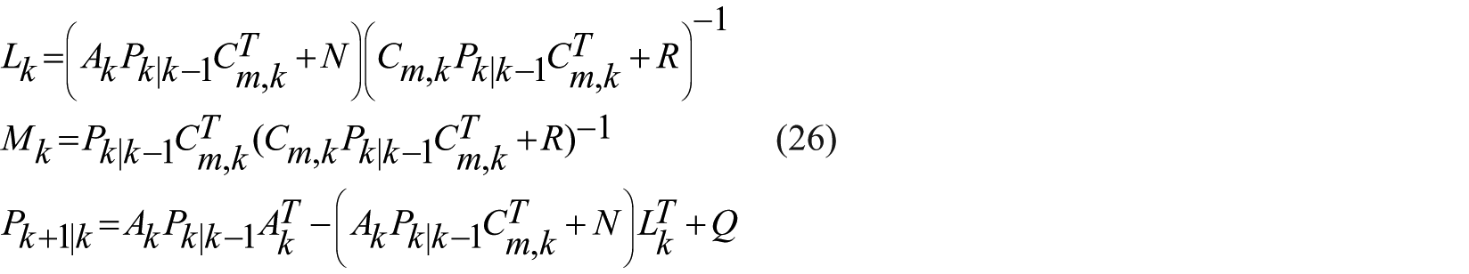
In equation (26), Q, R, and N matrices are constant covariance matrices and Ak and Cm, k are matrices depicting the state-space description of the system. The Pk|k−1 is the state estimate error covariance matrix at k constructed from the information from time k−1. Unlike the constant structure of the L and M matrices in the SKF, TVKF is constructed to update regularly the L and M matrices with the updated plant dynamics. Model updating strategy is a core issue in designing adaptive MPC controllers. Here, due to the parameter varying characteristics of the system, linear parameter varying (LPV) update law is selected. LPV systems are broadly used in various fields and industries ranging from chemical processes to robotics applications.42,43 An LPV system can be expressed as an array of plant models at specified operating conditions that can be used with adaptive MPC. An LPV system can be depicted in state-space form as follows

where x, u, and y are the state, input, and output vectors of the system, respectively. Matrices A, B, C, and D are parameter varying state matrices of the scheduling signal ρ(t), where ρ(t) T = [ρ1,…,ρnp] are time-varying parameters which are bounded in a predefined range.44,45 Let the bounds for the time-varying parameters be described as

With the definitions above, the procedure for the design of the AMPC system can be broken down into the following steps:
Step 1. The control structure of the robot consists of two loops. Outer loop controls the linear position and inner loop controls the angle of the COG. Inner loop dynamics are faster and the control mechanism naturally has more impact on the stabilization of the entire robot. AMPC design is applied to construct the inner control loop to stabilize the angle of the COG. The proposed system is a nonlinear parameter varying system and model predictive control (MPC) scheme requires a linearized model around operating conditions. Thus, an LPV system is created that includes three different linear plant models. Its parameter is ρ = m4, which changes with time since the fourth stick of the robot arm acts as a gripper picking up or dropping objects within the operating workspace.
Figure 17 shows the block diagram of the nonlinear robot system for linearization around the operating conditions as parameter mass m4 varies. The linearization process outputs three linear plant models which describe the local behavior of the system at specified mass values. Three linear models behave like LTI systems at 0.2, 0.3, and 0.4 kg, respectively, according to the design. LPV systems are used for updating the internal predictive model of the adaptive MPC controller. The block diagram of the LPV system obtained can be seen in Figure 18 .
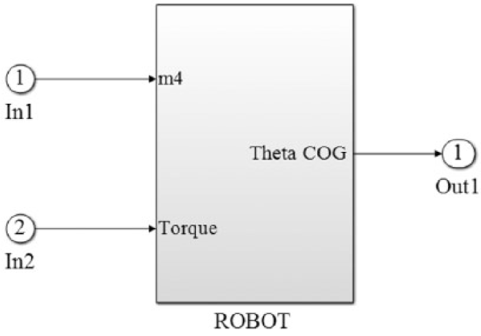
Linearization of nonlinear plant including varying parameter.
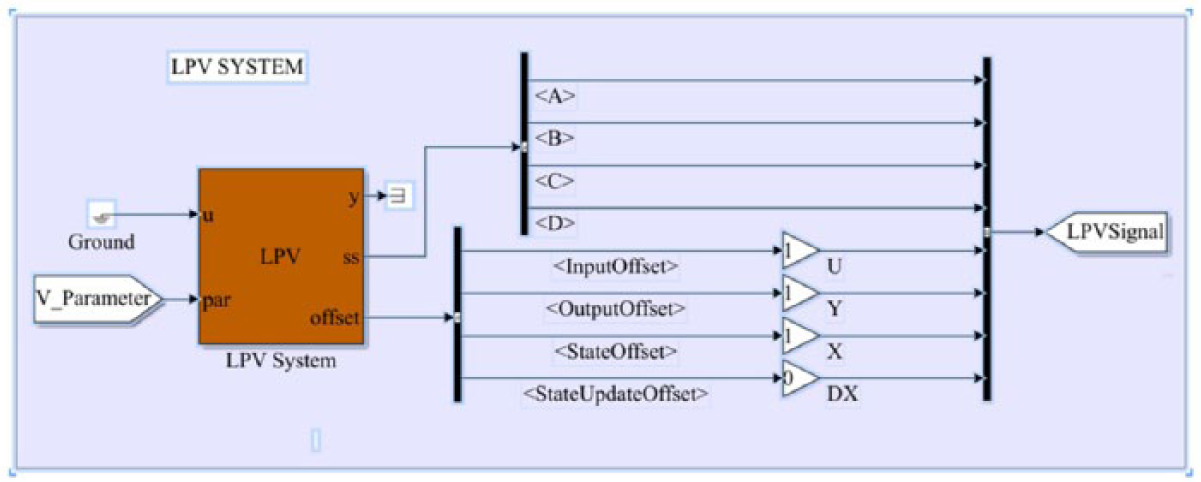
LPV modeling of mobile robot manipulator.
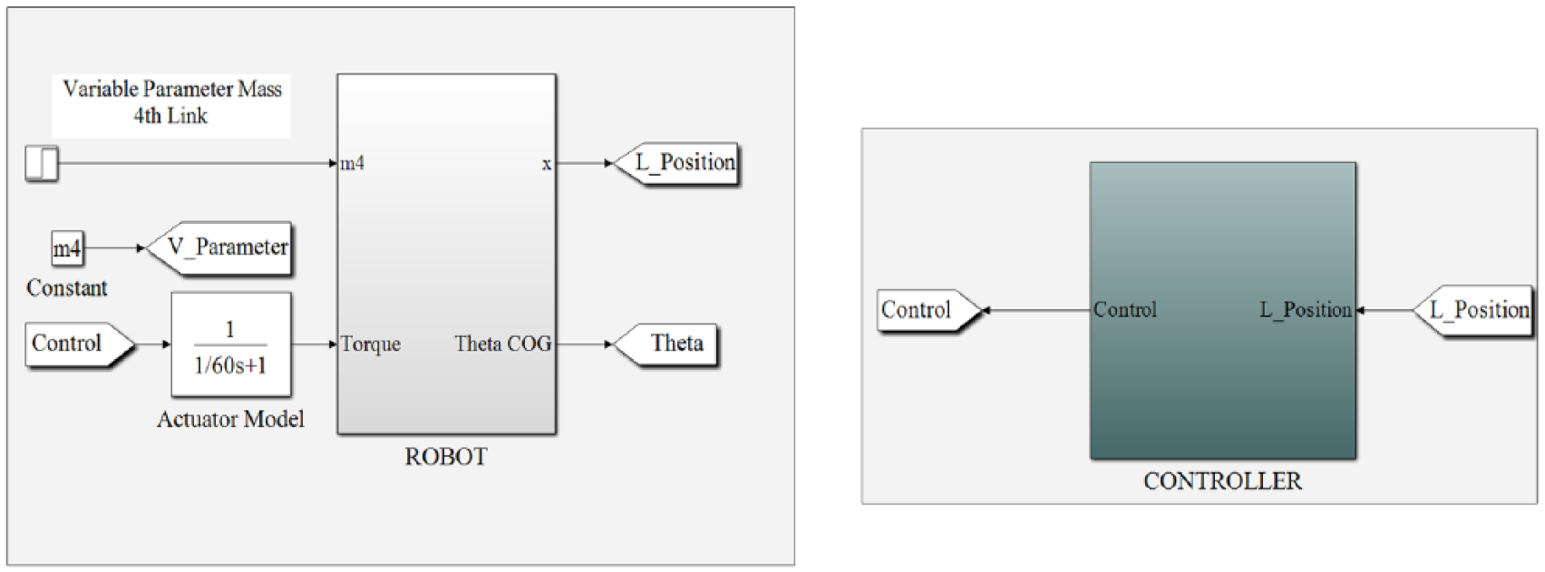
Step 2. After the LPV system is obtained, the AMPC controller is built. The general controller structure can be seen in the MATLAB/Simulink block diagram in Figure 19 . The design parameters of the adaptive MPC controller are shown in Table 8 .
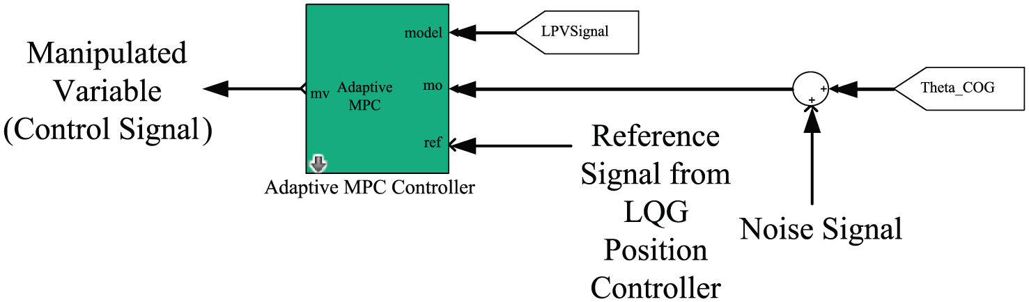
The angle control structure (inner loop).
Parameters of adaptive MPC controller.
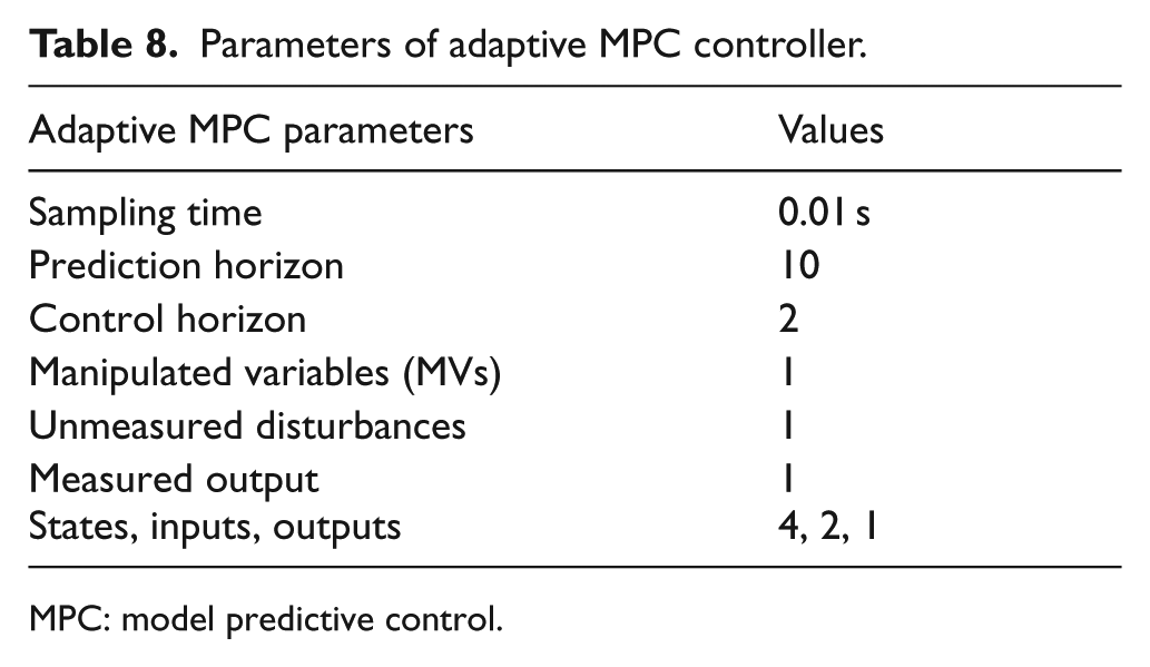
MPC: model predictive control.
Step 3. The stability and performance requirements of the angular dynamics are met with the adaptive MPC controller. The final step is designing an outer loop controller to create COG angle references to the inner AMPC controller based on the desired linear position. For that purpose, the LQG control approach is utilized. In principle, one could design another AMPC controller for the outer loop but this turns out to be overkill for this study. The linear position control in the outer loop is much slower and less demanding and hence a simpler and more standard LQG design was preferred, making this an AMPC/LQG controller overall. In order to design the outer loop LQG position controller, the system is linearized from the reference input (ref) of the adaptive MPC to position output of the system (x) as shown in the block diagram in Figure 20 .
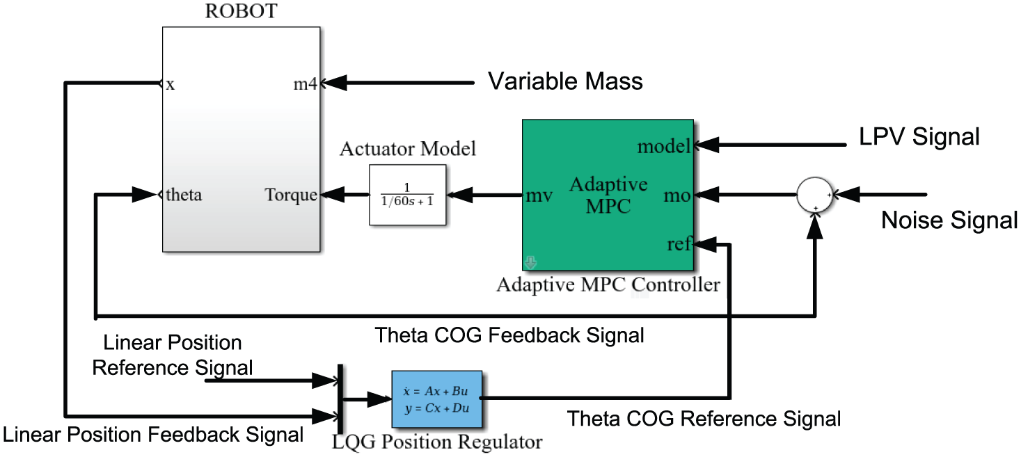
Entire control system.
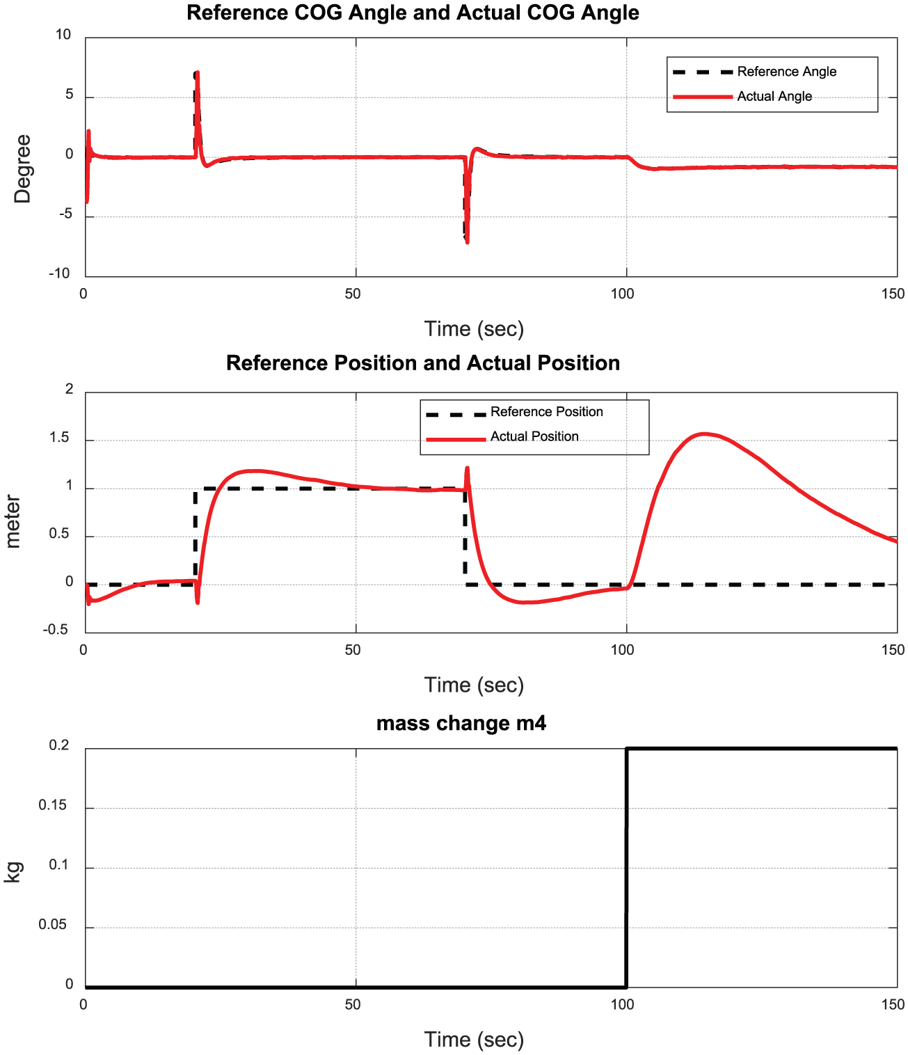
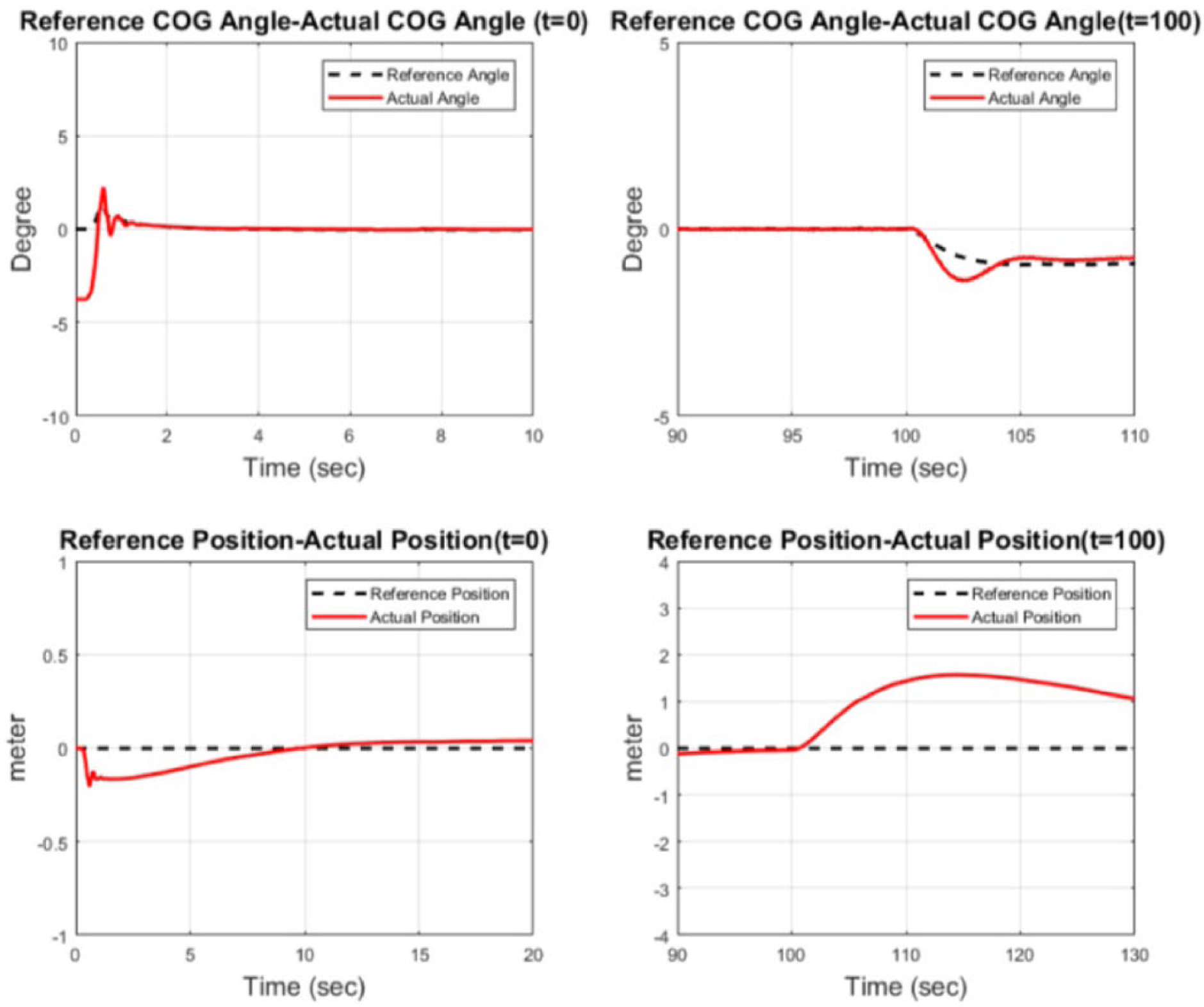
Once AMPC was designed following the three steps above, simulation studies were carried out under the same scenarios as in the PID/PID, LQG/LQG, and FBL/LQG cases in the preceding sections. The results are shown in Figures 21 – 23 . It can be seen that angular tracking performance is better than PID and FBL and similar to LQG, but slightly less oscillatory. The linear position tracking performance is fast and has no overshoot; as such it seems superior to PID, LQG, and FBL. Recovery from mass variation at t = 100 s is also better than PID, LQG, and FBL. The control effort is better than PID and similar to (but slightly more than) FBL and LQG. The performance metrics shown in Table 9 also support these statements. An additional plot for AMPC in Figure 24 shows the cost function converging quickly to zero, indicating a successful application of the method. Figure 25 shows the position tracking performance of AMPC and LQG on top of each other, for clarification of AMPC’s superior response.
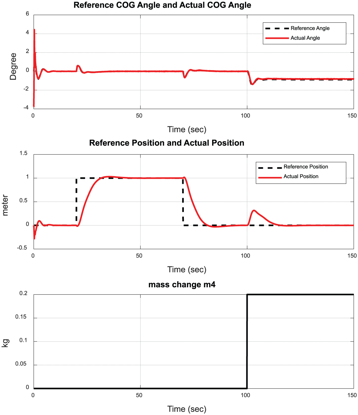
AMPC angular and LQG positional tracking with mass change.
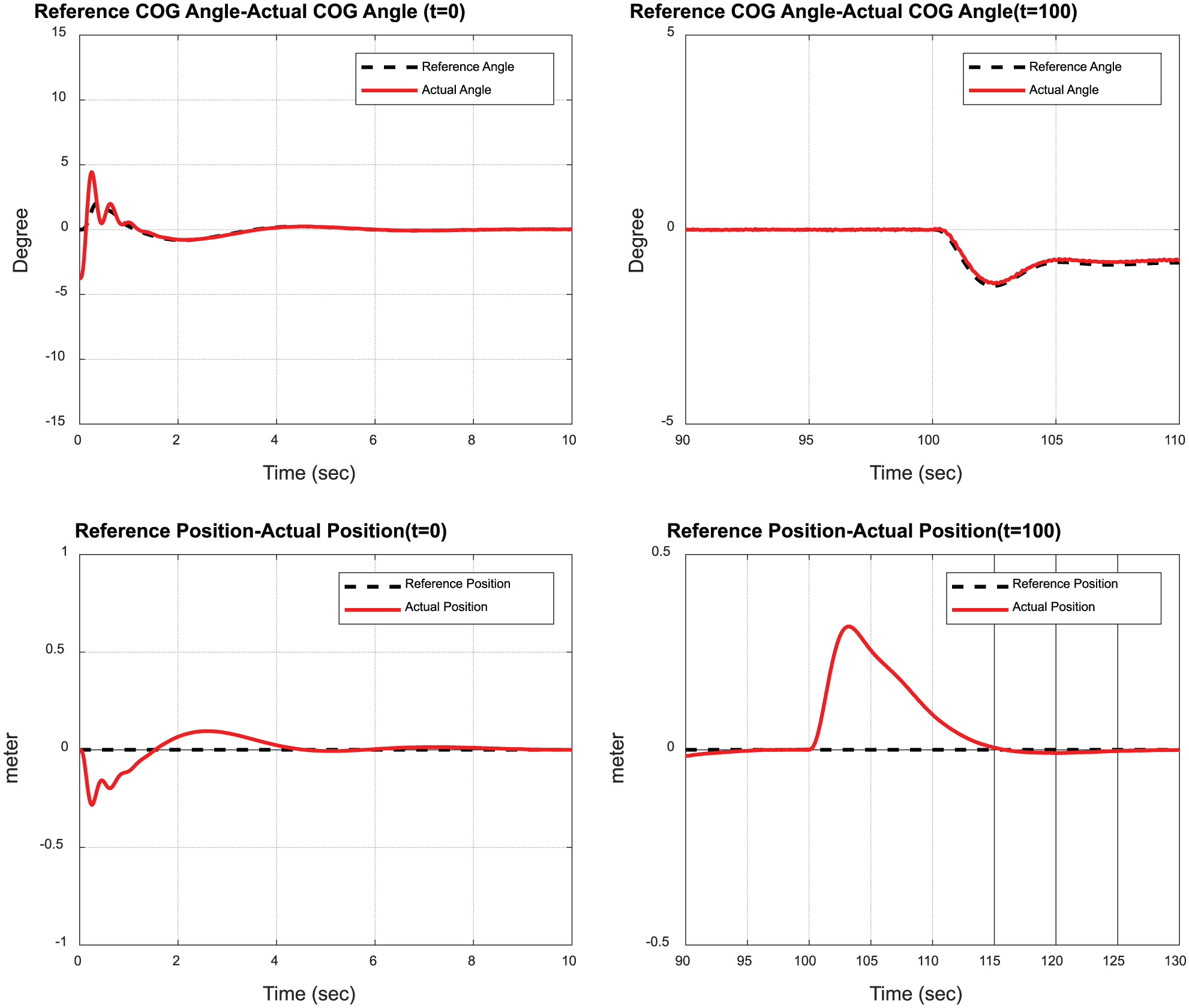
Transient and parameter change responses.
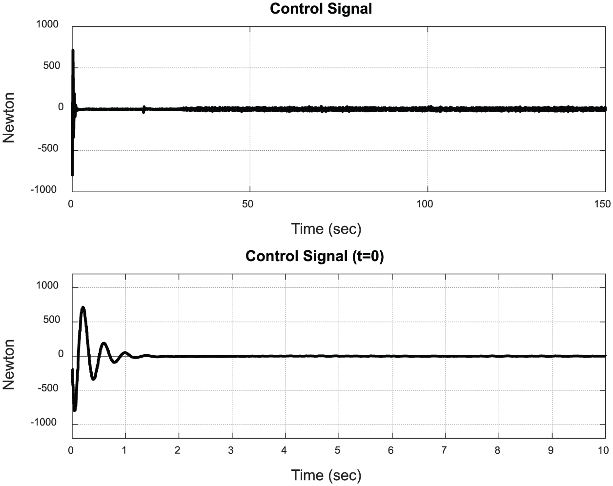
Control signal of AMPC.
Performance measures for AMPC scheme.
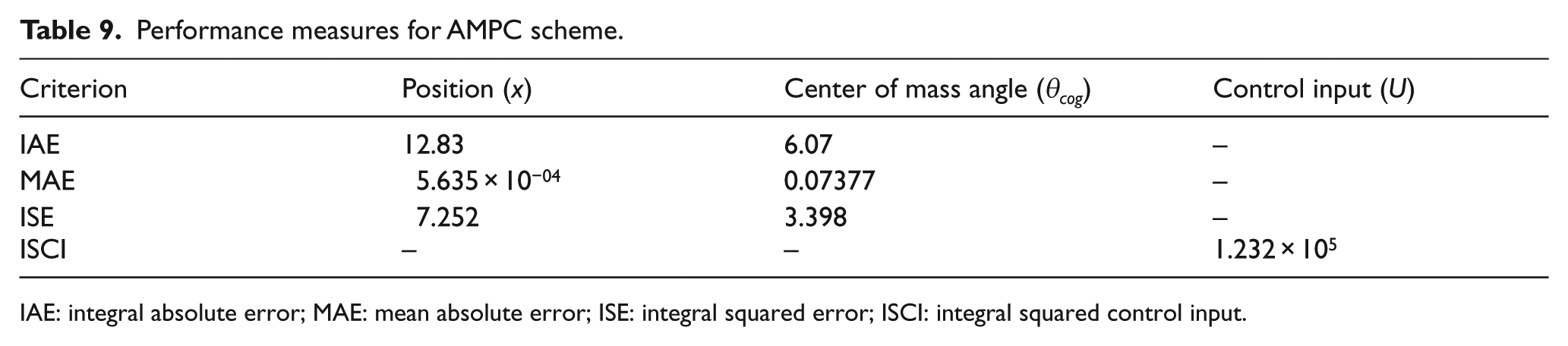
IAE: integral absolute error; MAE: mean absolute error; ISE: integral squared error; ISCI: integral squared control input.
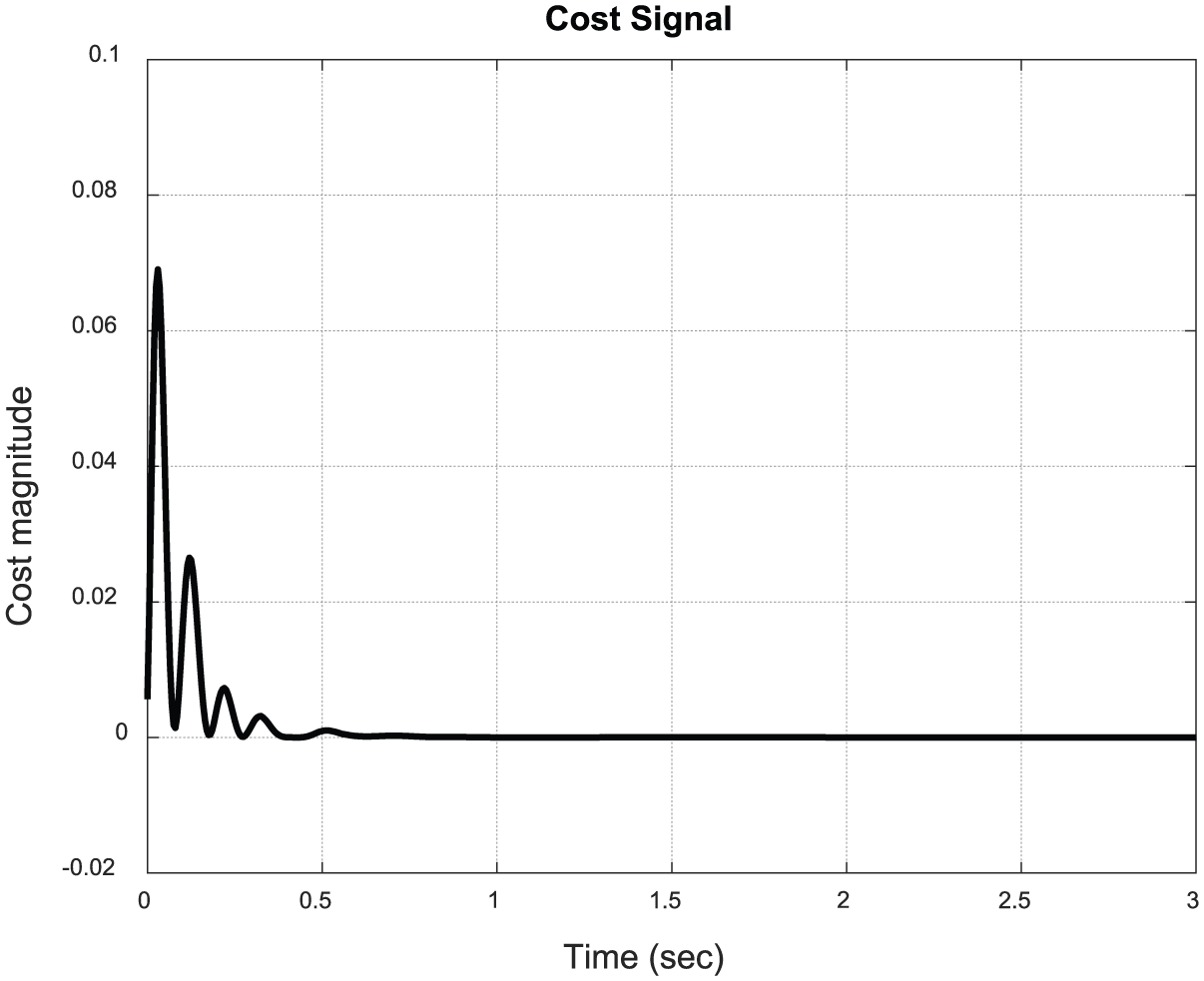
The cost function of AMPC controller.
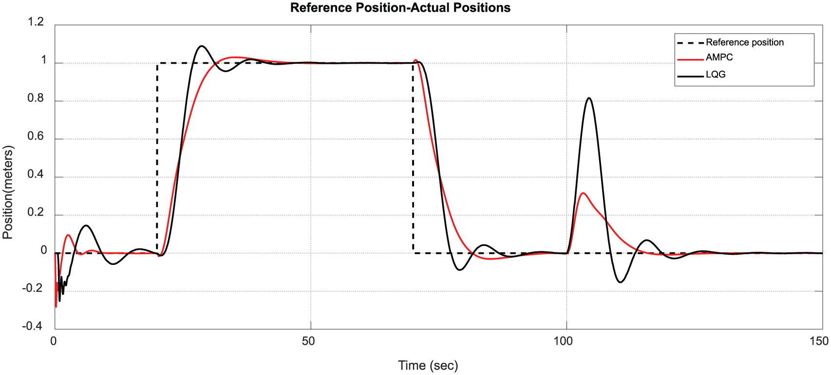
Comparison of AMPC and LQG control position tracking.
VIII. Conclusion and Future Works
This study implements adaptive model predictive control (AMPC) for a two-wheeled mobile robot in comparison to three standard control approaches, namely, PID, LQR, and FBL. A two-loop structure is utilized in all the approaches where the inner loops control the angle on the COG and the outer loop controls the linear position of the robot. The former is the faster dynamics and the latter is the slower dynamics. Apart from angle and position tracking, the controller is supposed to reject parameter changes due to mass variations, representing the manipulator picking up and dropping objects. The PID, LQG, and AMPC approaches are compared in terms of their reference tracking ability, control effort, and the metrics IAE, MAE, ISE, and ISCI. It is seen that AMPC shows superior performance in the majority of these categories and performs very well in the remaining ones, while showing good robustness to mass variations.
Investigating nonlinear control approaches for the two-wheeled robot platform is one of our planned future directions. We are also investigating the possibility of applying AMPC methods to other test platforms developed by our research group. These include improving the performance of flight stabilizer systems of fixed-wing aircraft48–50 and rotorcraft, 51 building better software-in-the-loop (SIL) and hardware-in-the-loop (HIL) testbeds,52,53 investigating novel approaches to provide robustness against parametric uncertainties, 54 and constructing specialized autopilots for control loss scenarios.55,56
Footnotes
Funding
This research received no specific grant from any funding agency in the public, commercial, or not-for-profit sectors.