
Abstract
A method for detecting leaks in plastic water supply pipes through analysis of the pipe’s surface vibration using a high signal-to-noise ratio accelerometer is proposed and examined. The method involves identification of the changes in vibration frequencies caused on the pipe by the leak and is developed from and examined with respect to detailed experiments. The results are promising, showing that leak detection in plastic pipes is possible provided that the sensor is placed at a small distance from the leak, since wave attenuation in plastic is strong. The results indicate that the methodology has the potential to be a new and competitive type of mobile leak detection system.
I. Introduction
Detecting leaks in water supply networks is becoming an issue of great interest since clean water supplies tend to decrease and supply prices increase accordingly.
So far, satisfactory results in detecting leaks have been obtained only for metal pipes since the acoustic signals generated by the leak are easily transmitted to a sensor, are wide band, and of high frequency.1,2
As recent studies have shown, leak detection in plastic water filled pipes can also be obtained by vibration analysis and, more specifically, by use of hydrophones, acoustic emission sensors, and accelerometers connected onto the pipe’s surface.3–5
Most water supply networks nowadays are made of plastic pipes either entirely or a large portion of them, creating a need for novel and efficient ways to detect leaks in these types of pipes.
In order to detect a leak on a plastic pipe, an approach that incorporates a high signal-to-noise ratio is proposed in this paper. The method used involves identification of the frequencies caused by a pipe with flowing water and a leak and their analysis, in contrast with the frequencies produced by a flowing water pipe of the same features, yet without a leak, given that the vibration frequencies of the specific pipe when leaking are already known or can be measured.
Leakage detection in water supply networks is also closely related to seismic activities. Real-time vibration monitoring of water pipes provides a valuable tool for identifying leakage that might occur from seismic phenomena. It is not rare for leaks to be created as a result of earth vibrations and earthquakes. Being able to monitor pipeline vibration activity can provide feedback on both pipeline reaction and seismic analysis. In this paper, the first case is explored.
A. The experimental setup
The sensor
The accelerometer used is the KB12(VD) from IDS Innomic. It is based on a very sensitive piezoelectric sensor with an integral amplifier (IEPE type) that ensures low noise over a wide frequency range (Pictures 1 and 2).
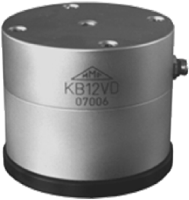
The Innomic IEPE KB12(VD) piezoelectric accelerometer.
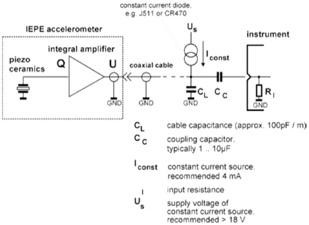
General IEPE type sensor connection scheme.
Signal conditioning—PC interfacing
The Innobeamer LX2 USB sensor interface was used for signal conditioning and analog-to-digital conversion, sending the digital values to a PC through a USB2.0 port (Picture 3). It was selected for its high resolution (24 Bit) in high sampling rate (8 KHz) and its high accuracy (<2%).

The Innobeamer LX2 USB sensor interface.
The software
The software used was the VibroMatrix, which is recommended by Innomic as the proper software to make full use of the high capabilities of the KB12VD piezoelectric accelerometer.
IEPE sensors are directly connected to sensors with charge output by an in-line charge amplifier to the InnoBeamer. InnoBeamers transmit the sensor data by a USB interface; they are supplied by a USB interface as well. Instruments display the required information about the vibration state in real-time on the screen.
The following Vibromatrix modules were used:
InnoPlotter—digital strip chart recorder for vibration parameters;
InnoAnalyzer—frequency and vibration analyzer.
The setup
A plastic polyethylene pipe 30 m long with 32 mm outside diameter, 28 mm inside diameter, and pressure rating PN6 was fixed in a narrow channel (10 cm wide) at low depth (15 cm), which was later covered with soil.
One end of the pipe was connected to the water supply network by means of a plastic connector, while the other was connected to a valve that allowed the pipe to be either left open in order not to affect the water flow, or closed so that no water was allowed to flow (Picture 4).
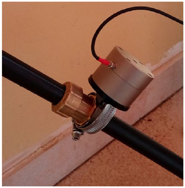
Accelerometer setup.
In a position close to the water supply connection (25 cm) the piezoelectric sensor was placed by means of a metal nut attached firmly to the pipe (Picture 5). 6
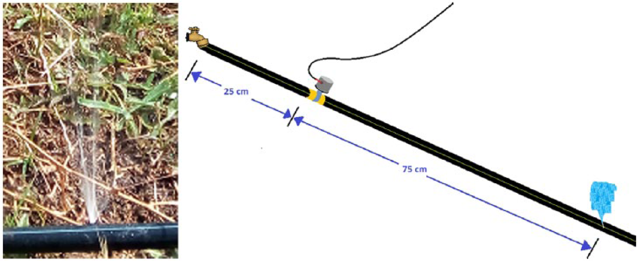
Pipe leak photo and schematic.
The experimental procedure
First stage. The full range of the frequencies produced by the pipe vibrating due to the water flow was recorded in a period of 20 s at 1 kHz sample rate.
Second stage. In a position close to the water supply (1 m), a hole 2 mm in diameter was created with a screw mimicking the leak and the corresponding water flow.2,7
Again, the full range of the frequencies produced by the pipe vibrating due to the water flow and the leak water flow was recorded in a period of 20 s at 1 kHz sample rate.
II. Data Analysis
The data collected from the accelerometer were divided into separate categories. The first categorization was in terms of whether there was water flowing in the pipe or not, and the second categorization had to do with whether there was a leak in the pipe or not. The above resulted in four signal cases that are presented in the table below with their corresponding acronyms:
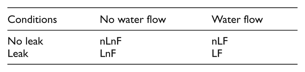
Throughout this paper, the above acronyms are used in order to characterize a signal, depending on the conditions used when acquiring it. The goal of this study is to produce a system that will be able to distinguish successfully whether there is a leak in a signal or not, given the leak waveform, regardless of whether water is flowing or not.
The accelerometer setup records the acceleration of the plastic pipe’s external surface. In cases in which the acceleration values alone were not distinct enough in order to characterize the signal, frequency analysis was used, in terms of fast Fourier transformation (FFT), power spectral density (PSD), cross power spectral density (CPSD), and wavelet transform (WT) analysis. 6
The graphs in Figure 1 present the acceleration values for two of the above cases. No Leak No Water Flow and Leak No Water Flow.
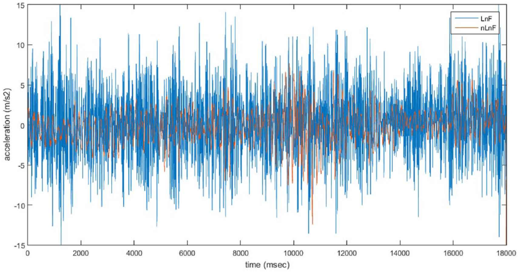
Leak no water flow (blue) and no leak no water flow (orange) acceleration graph.
This is an obvious case where the amplitude of the Leak signal is overall significantly higher than the amplitude of No Leak, in the No Water Flow case. 8 A system that monitors acceleration values of a water pipe will easily identify the difference in acceleration values when a leak occurs. In addition, this difference will be constant as time progresses. Therefore, the leak will be detectable by the system, given that No Water is flowing in the pipe. 9
We consider that the above scenario, although it produces good results in the laboratory, is only viable in real-life scenarios in small-diameter pipes near the private customer’s end, where continuous water flow is highly unlikely to occur. In main water distribution networks, however, water will, most likely, be flowing constantly. Thus, further examination is required for distinguishing leakage in water flowing pipes.
Figures 2 and 3 show the acceleration values of the LF and nLF signals for a 10 s duration. It is clear that the leak itself cannot be easily distinguished when water is flowing, because the vibrations produced by the water flowing itself exceed the vibrations produced by the leak alone. To overcome this boundary, we use frequency analysis.
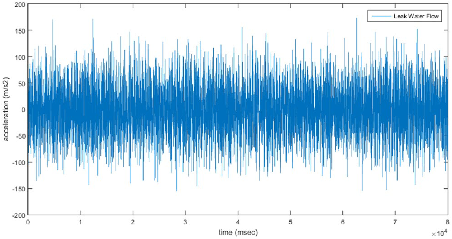
Leak water flow acceleration graph.
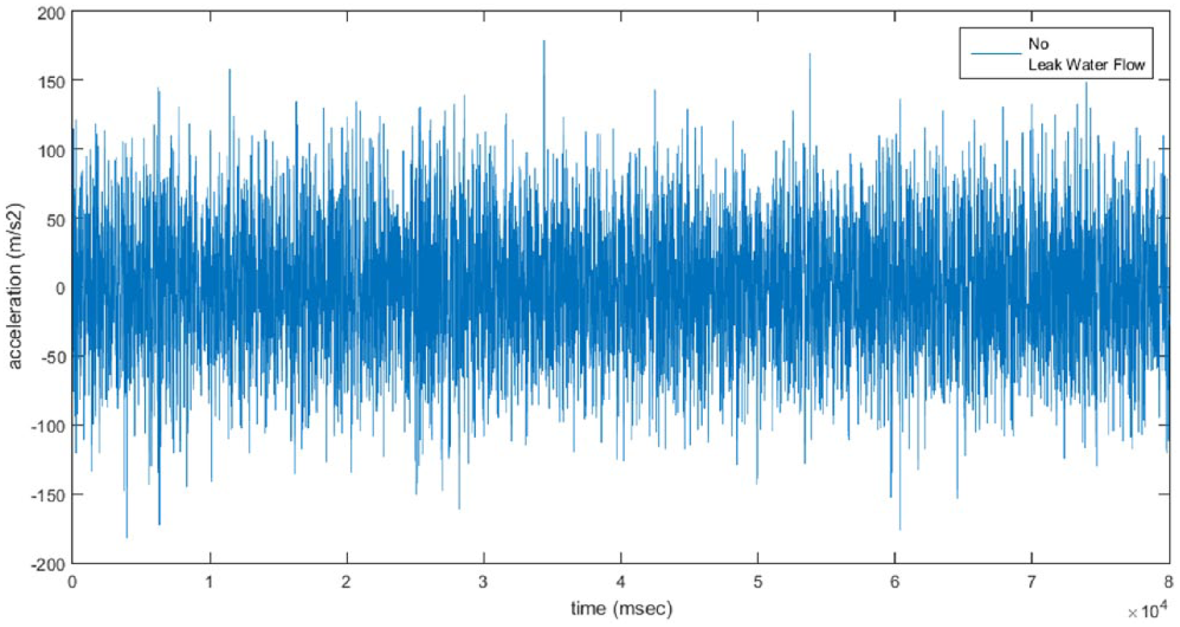
No leak water flow acceleration graph.
A. Fast Fourier transformation
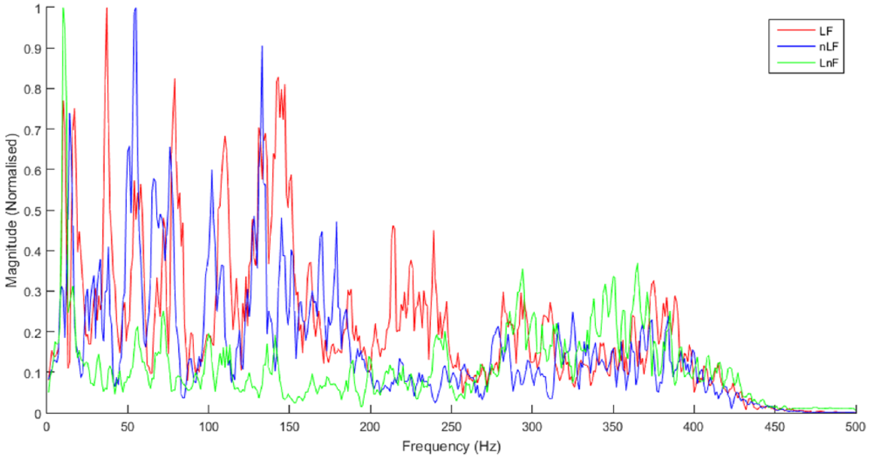
The idea is that by analyzing the frequency content or the time-frequency content of the Leak No Water Flow signal, we may be able to locate the specific frequency behavior in the Water Flowing signal. 10 Toward this, we first built a system with MATLAB, which splits the original signals into random 1 s parts. It uses FFT to produce the corresponding frequency waveforms for the three signals at hand: LF, nLF, and LnF (Figures 4–7). It then extracts the local maxima of the FFT graph for the three signals and compares them. It creates a score for LF and LnF signals, depending on how close their local maxima are to the nLF signal. Depending on the score, the system is capable of concluding which of the input signals has a leak.
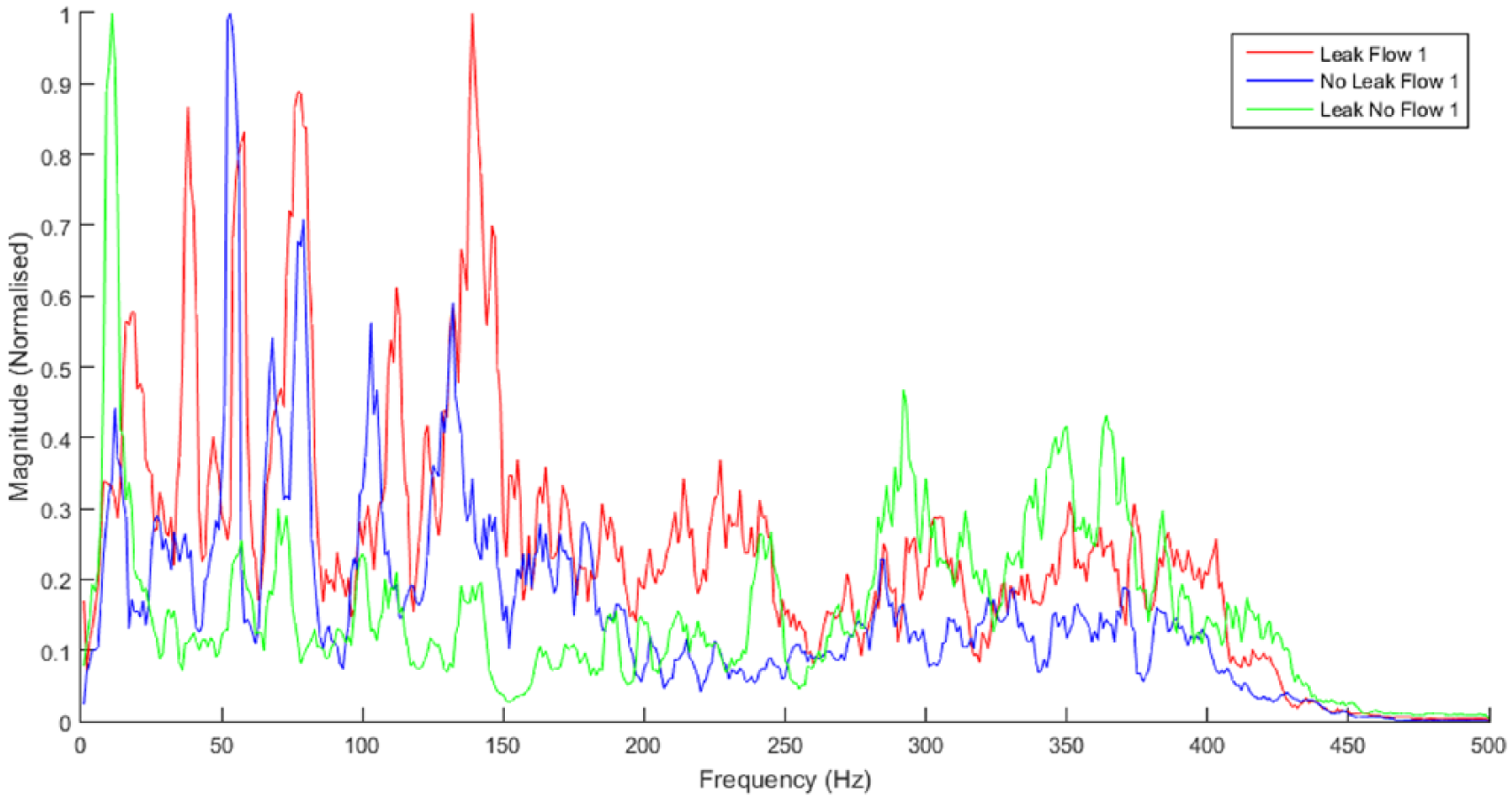
Example 1—FFT.
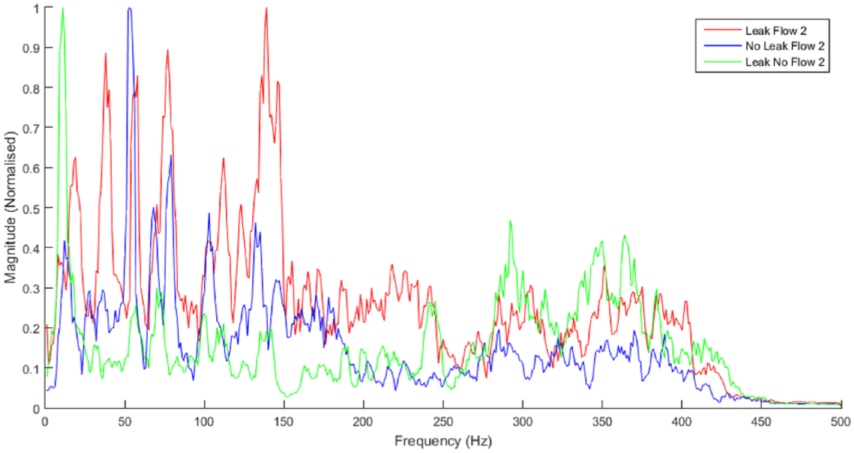
Example 2—FFT.
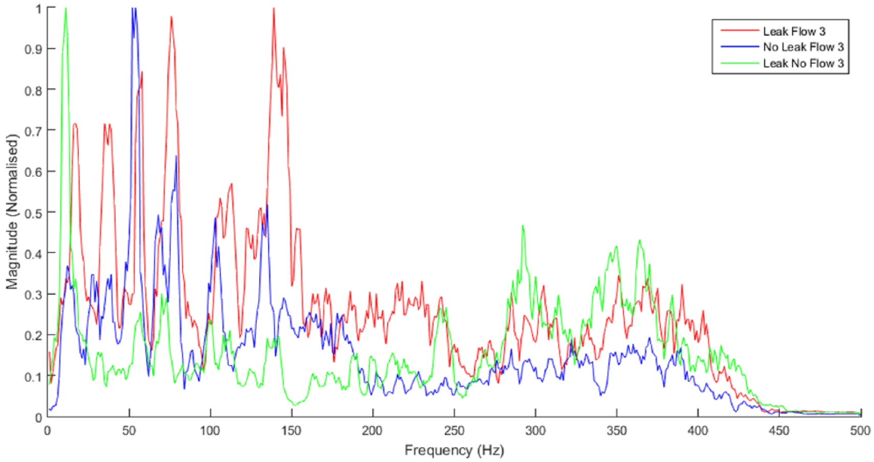
Example 3—FFT.
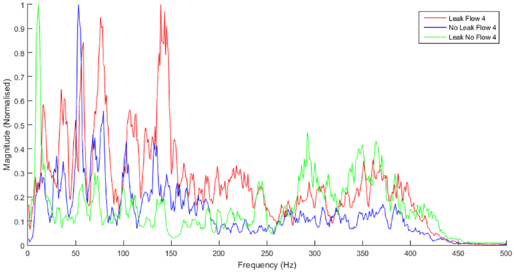
Example 4—FFT.
By examining the above graphs, one can easily notice that the Leak signals have a clear increased frequency activity in the area 270–370 Hz, whereas the signals with No Leak present show low activity in this region. A closer look at the green line (Leak No Flow) reveals that this region is exactly where the Leak can be found, given that this is a clear signal of Leak with no other external vibrations produced by the flowing water. The signals that were acquired during water flow have a lot of activity in other regions as well, which is caused by the vibrations of the pipe from water flowing inside. At this point though, it looks as if the 270–370 Hz region is present in high amplitude frequency only on Leak signals, so that it can be determined as a criterion of whether an acquired signal from an accelerometer contains a leak.
B. Cross power spectrum
Another method used for recognizing the leak in a signal is the CPSD, using the CPSD function in MATLAB. Cross-spectral analysis allows one to determine the relationship between two time series as a function of frequency. PSD is the distribution of power along the frequency axis. Cross-spectral density is the same, but using cross-correlation, so one can find the power shared by a given frequency for the two signals. Running CSPD for LF-LnF and nLF-LnF we were able to pinpoint that in the frequency area where the leak is present, the CSPD graph had higher values for the LF-LnF than for the nLF-LnF, which proves a leak is present on the LF signal.
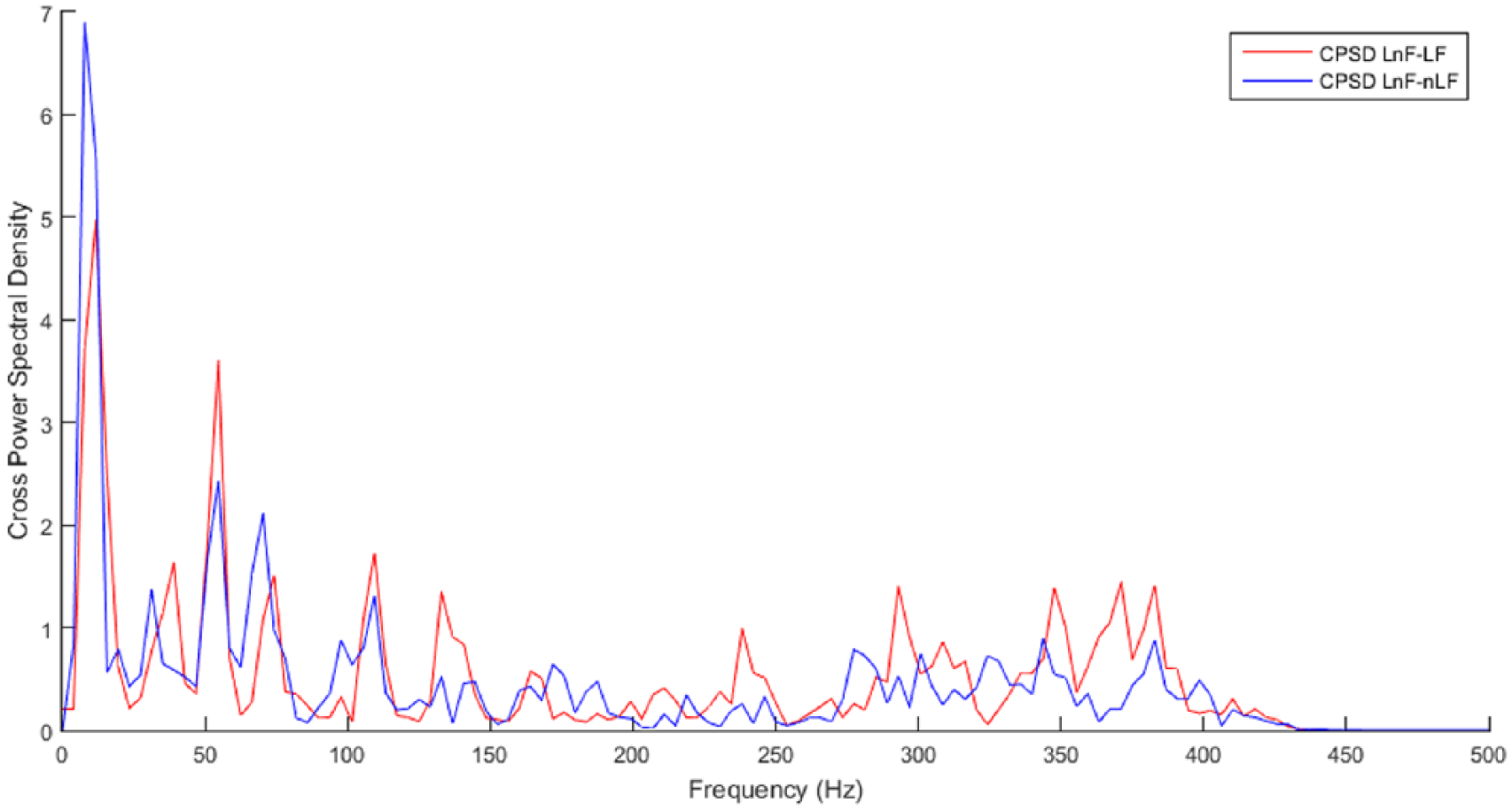
The next step in our investigation is to confirm the above results using another method. 11 In this case, we used the CPSD between signals using the CPSD function in MATLAB, as shown in Figures 8–11. This function compares the frequency content between two signals in terms of energy distribution, and returns a graph. Higher values mean more signal similarities in the specific frequencies.
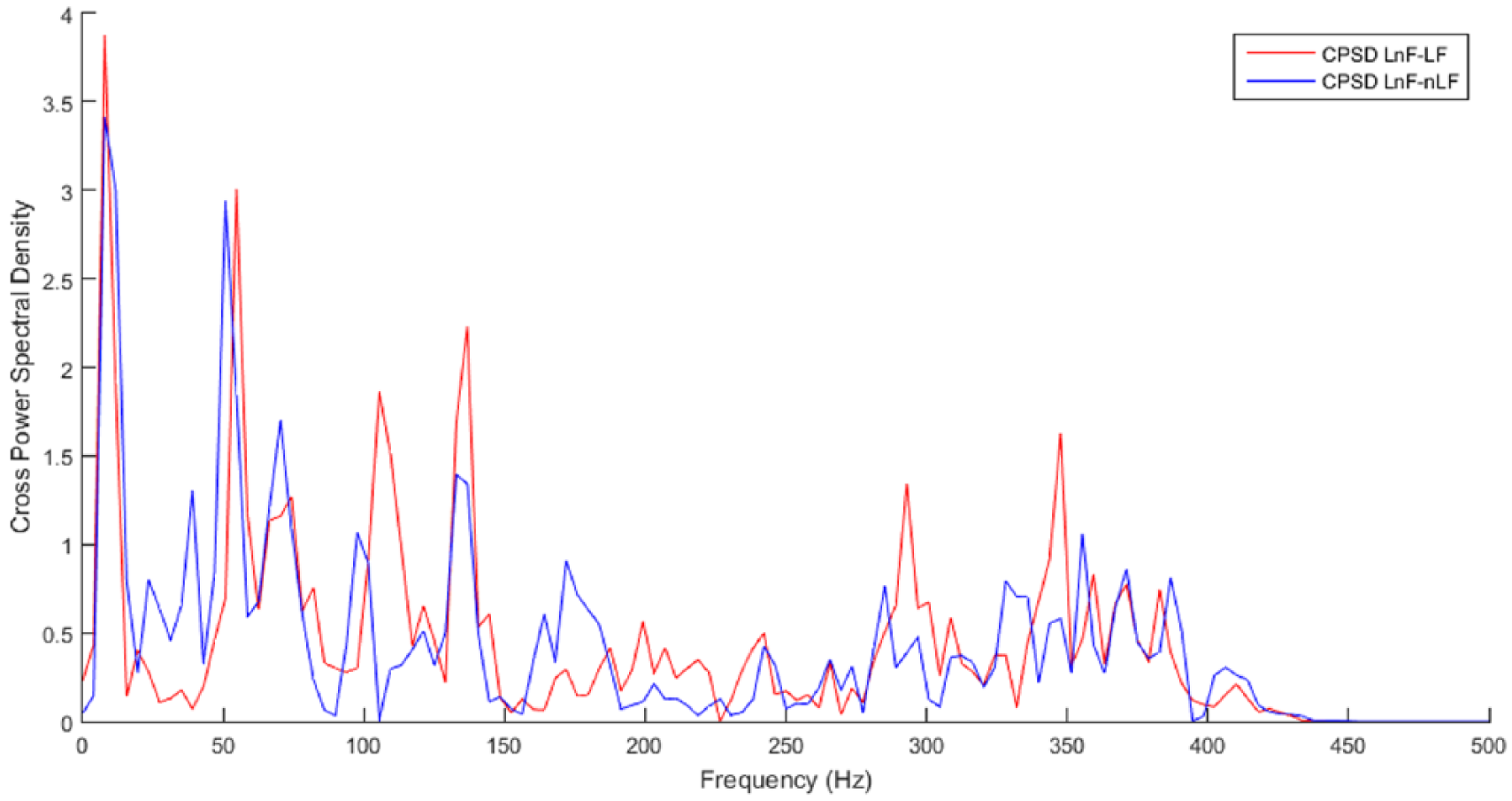
Example 1—CPSD.
Example 2—CPSD.
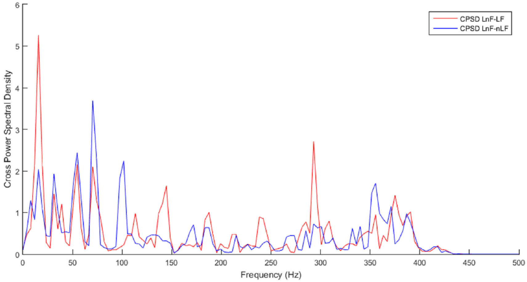
Example 3—CPSD.
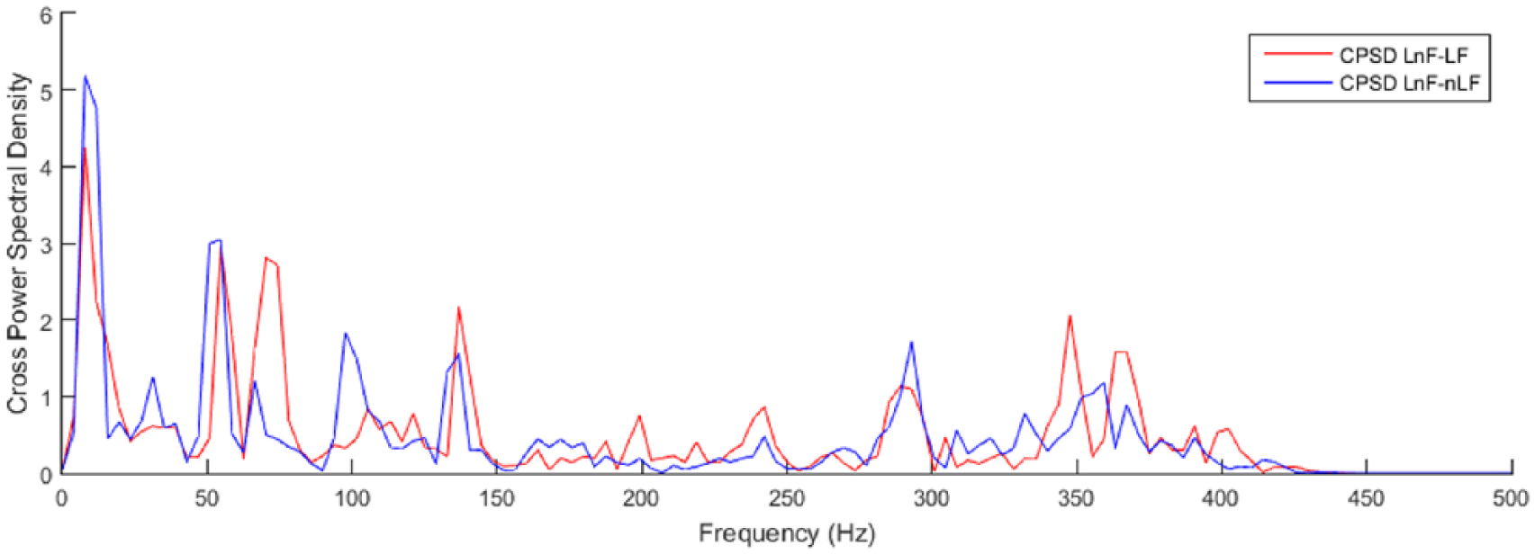
Example 4—CPSD.
The red graphs represent the cross-spectral density between Leak No Flow and Leak Water Flow, whereas the blue graphs are the CPSD between Leak No Flow and No Leak Water Flow. It is clear from the above that in the same area 270–370 Hz that we spotted frequency activities on the Leak signals from the FFTs, there are also higher CPSD values between the same signals. In this case, it is safe to conclude that the specific type of plastic pipe produces vibrations when leaking in this frequency area. By monitoring vibrations and calculating the FFT of a given signal, the proposed system can detect possible leak by calculating the differences in frequency content at the specified range over time.
C. Automating the process
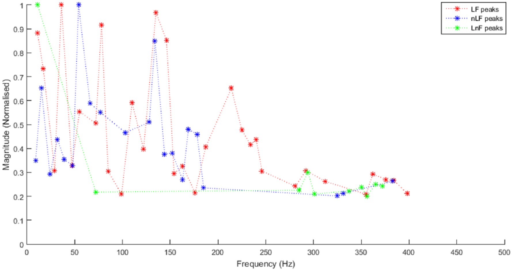
Taking this into account, we generated a MATLAB code that takes as an input a random 1 s duration time signal from the pool of recorded material with the above setup for all three types of signals. Given the Leak No Flow signal, it tries to distinguish which of the other two signals has a leak present. It calculates the peaks of the normalized FFTs and it provides a score based on the number of peaks in the FFT graph that are in the same range of frequencies as the Leak signal. A higher score means that the given signal’s FFT has peaks in the same frequencies (with a tolerance) as the Leak signal, as shown in Figures 12 and 13 . This code has a very high success rate and it provides a valid answer to which of the input signals corresponds to a case with a leak. It is important to note at this point that the system’s success rate is limited by the fact that there should be Leak No Flow signals available in order to train the system beforehand. Below is an example of random signals using the described system:
Score A: 10;
Score B: 6;
Conclusion: Signal A (LF) has a leak.
Example 5—FFT.
Example 5—FFT peaks.
The FFT graphs presented above were smoothed using MATLAB’s “smooth” function:
Pa1_smooth = smooth (Pa1, s, “moving”)
with moving average algorithm and smoothing distance s = 3.
Then they were normalized by dividing with the maximum number present in each graph.
Pa1_norm_smooth = Pa1_smooth/max(Pa1_smooth)
This is because we are currently interested in the shape of the frequency pattern, not in absolute values.
The peaks were calculated using MATLAB’S “findpeak”
[pksPa1, locsPa1] = findpeaks(Pa1_norm, “MinPeakHeight,” 0.2, “MinPeakDistance,” 5)
with MinPeakHeight = 0.2, and MinPeakDistance = 5
Then we used the “ismembertol” function, which returns an array containing 1 (true) where the data in A is found in B, but with tolerance. Tolerance used is 0.05.
CA = ismembertol(locsPc1, locsPa1, 0.05)
Running more examples with this test code in random 1 s signals we had a high percentage of success in identifying the leak signal.
More specifically, we ran the automated process in 20 random 1 s samples and we had a 95% of success in identifying the leak.
The MATLAB code used for the above process is available on request.
D. Wavelet analysis
The signals were also processed with wavelet analysis using a biorthogonal spline filter as the wavelet family. Figure 14 shows the WT in timescale space, for the cases in the same order as the table in section “Data Analysis.” It is obvious that the nLnF case ( Figure 14(a) ) is easily distinguished from all other cases, and so is the nLnF case (Figure 14(b)). The LF case contains much energy (in terms of the wavelet transform) at mid-scales, which the nLF case does not. It is noted that the values of the wavelet coefficients larger than 200.0 are chopped in Figure 14(d) so direct comparison to the rest of the figures in Figure 14 can be made (i.e. in the range 0.0–200.0). Figure 15 shows the entire range of values in Figure 14(d) , illustrating further the high energy at mid-scales, which makes the LF case distinguishable from the nLF case. The total energy of the WT (summation of the square of the wavelet coefficients) at mid-scales is significantly higher for the LF case than for the nLF case.
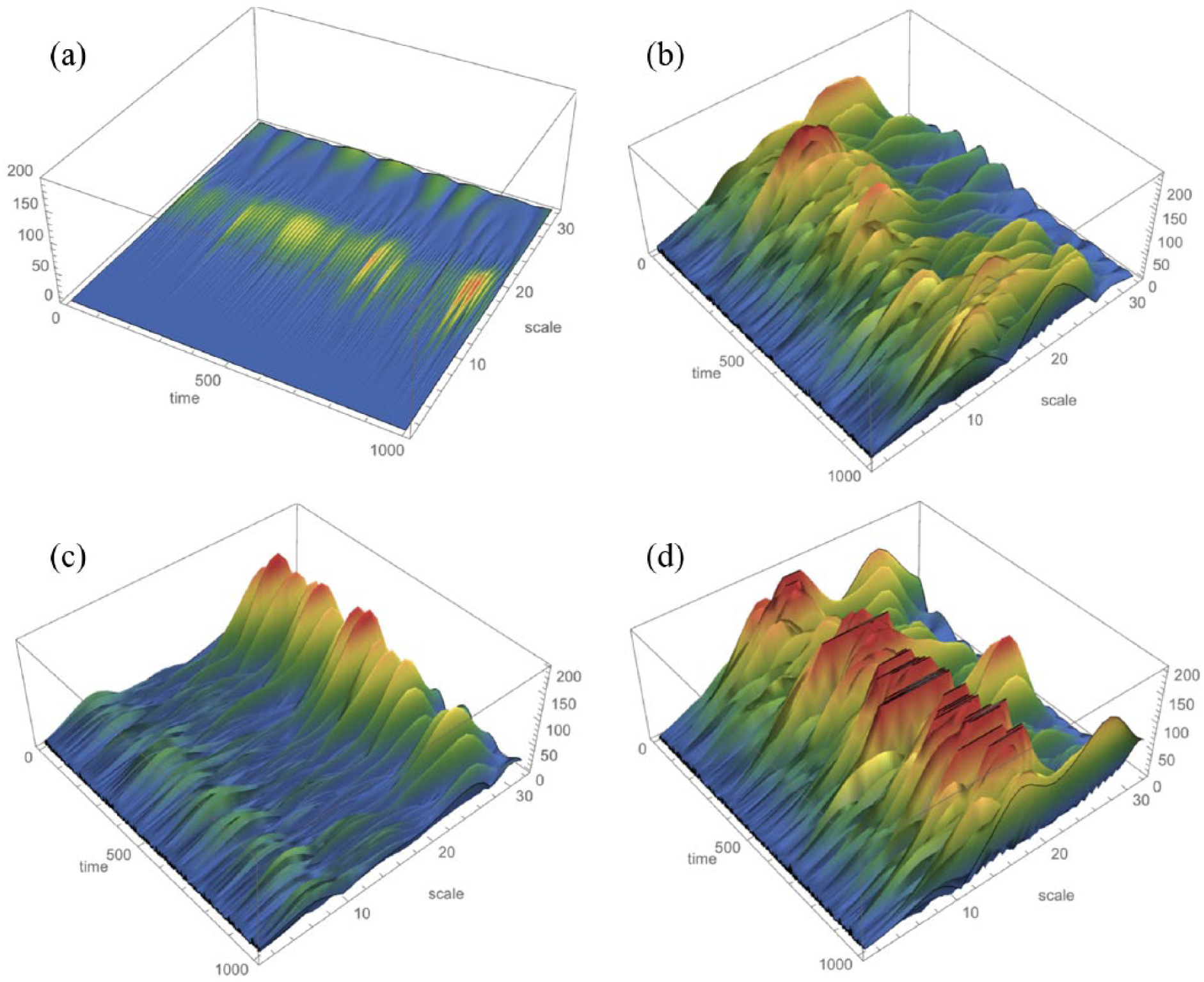
Wavelet coefficients in timescale space for (a) nLnF, (b) nLF, (c) LnF, and (d) LF.
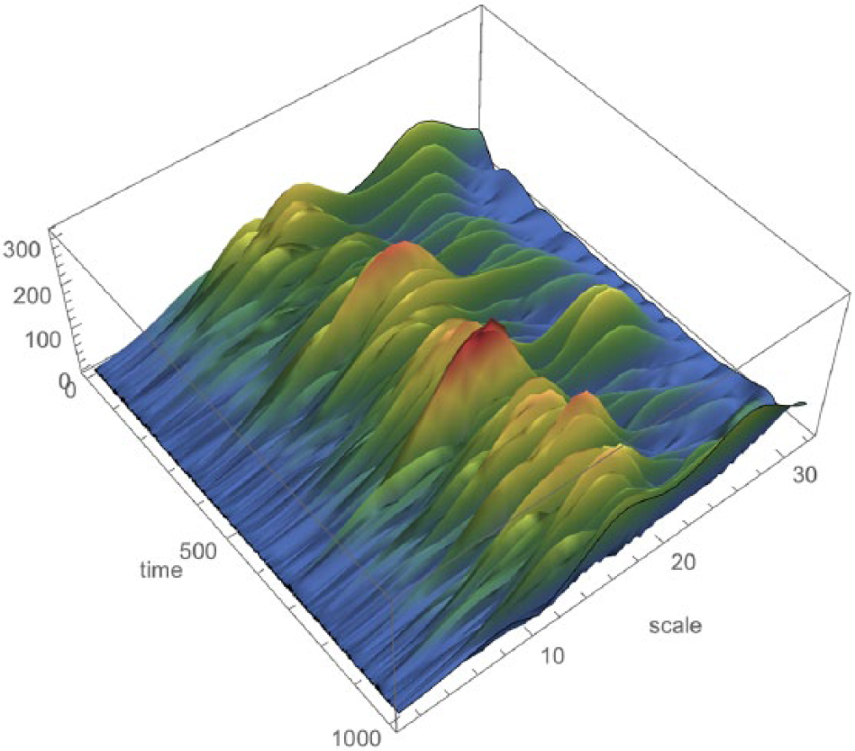
Same as Figure 14(d) , but for all ranges of values shown.
Wavelets are able to decompose signal information into a range of spatiotemporal scales so that the signal content can be stripped out of external noise factors. This, of course, considers that external noise manifests itself at low amplitude at the scales used primarily for detection of leaks. In other words, if the WT of the external noise has high magnitude relevant to that from the flow at specific scales, that is, the scales used predominantly for detection of leaks, then there is a problem of severe interference from the external noise. However, the noise at such scales is small as can be concluded from the specific results reported in this paper.
III. Conclusion
Vibration analysis of plastic pipes using high-sensitivity accelerometers can lead to long-term leakage detection. As shown, there are cases, for example, Leak with No Flow, where the vibration amplitude itself can show if a leak is present. The vibration caused by the leak on the pipe surface has higher acceleration values than any other vibration source coming from noise or other factors. The difference is detectable and constant in time, showing that it could not be caused by random external factors, other than a leak.
For the rest of the cases, where the leak cannot be directly detected by the difference in acceleration amplitude, and the vibrations caused by the flowing water overwrite the vibrations from the leak, the leak can still be detected by vibration analysis in the frequency domain. This paper shows that given a sample of clear leak vibrations on a specific pipe, the system can be trained in order to detect similar frequency behavior in real conditions and decide whether there is a leak or not. Training the system with leak signals a priori is essential, however.
FFT is also essential for providing the frequency area that the Leak No Flow signal is present. The system provided very good results by comparing the FFTs of observed signals. CPSD was used, similarly to wavelet analysis, in order to confirm the FFT results using other methods.
IV. Future Work
The future work includes experimenting with different pipe lengths and different pipe thicknesses in order to investigate the effect of these parameters in the frequencies produced.
Other parameters that should and could be investigated in the future are as follows:
The depth inside the soil where the pipe is placed, the type of pipe fixture used, and how these can affect the leak detection procedure (type of material used—number of fixtures per meters of pipe);
The hole patterns (e.g. cracks—holes—other patterns) and the hole diameter.
Another hypothesis to be tested in the future is whether the sensor can be placed on the surface of the ground while the pipe is some distance (e.g. a few centimeters) underground, thus creating a mobile leak detection system.
Another important factor to be taken into account in future studies is the extension of the current system so that it is able to detect a leak straight from a continuous signal, while the leak was not initially present, but occurred at a later stage. Being able to detect the leak without comparing the signal’s frequency behavior with a clear Leak signal would be the last step in applying the algorithm to real-life conditions.
The main code of the proposed algorithm is based on FFT comparison, but given that CPSD and wavelet analysis confirmed those results, a similar algorithm can be developed in the future that will compare CPSDs.
Moreover, FFT is related to one signal, while CPSD is referred to the relation of two different signals in terms of cross power per frequency. As a result, a more sophisticated approach should be considered in a future study for CPSD comparison.
Different types of sensors can also be tested like new high-sensitivity MEMS sensor as MEMS technology is progressing rapidly, enriched with wireless technologies. 12
The system described in this paper presents the ability to detect a leak on a pipe, given the clear leak waveform of the specific pipe type. In order for this system to be used for every pipe type in real-world applications, a formula can be created that would calculate the waveform or the frequencies that would be expected from leakage at every pipe type available in the market. Another approach would be the precalculation of leakage frequencies in several pipe types so that a table will be created that will be used as an index of the expected frequency behavior in several plastic pipes, as has already been done by Atkins et al. 13 for a variety of metal pipes.