Sage Journals: Discover world-class research

Abstract

My previous article on ‘Setting the parameters of proportional–integral–derivative controllers’ looked at the initial work of Ziegler and Nichols and how their concepts have developed into today’s proportional–integral–derivative controllers in the process industries. Here, I look further into the increased control possibilities the controller provides when used in the slightly modified form of a proportional–integral controller with proportional–derivative feedback.

I. Introduction

Towards the end of my previous article on proportional–integral–derivative (PID) controller settings,¹ I had a section headed ‘Further Comments on PID control’, which contained the following two sentences:

A pure D term is never used as theoretically it gives an infinite gain at high frequency. It is normally replaced by $s T_{d} / (1 + α s T_{d})$ with α typically less than 0.1. This term is also often fed from the process output rather than the error to avoid the ‘derivative kick’, since a step change in set point of, say r, produces a step change in error which if fed to $s T_{d} / (1 + α s T_{d})$ gives an initial output of $r / α$ .

Using a terminology which I have used for several years,² I have called this form of PID control PI-D, to denote that the D term is fed from the output. In this article, I want to say more about what I believe are additional benefits of this implementation and also of a further extension to a PI-PD format, that is, with the feedback term including a proportional term as well as a derivative.

II. PI-PD Control

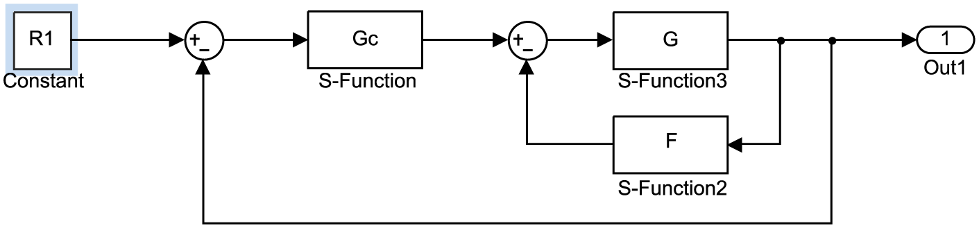
Figure 1 shows a feedback loop where the controller consists of two transfer functions G_c in the error channel together with a feedback through F from the plant output. In ‘classical’ PID control, F is unity and $G_{c} = K [1 + s T_{d} + (1 / s T_{i})]$ ; in PI-D control, $F = s T_{d}$ and $G_{c} = K [1 + (1 / s T_{i})]$ ; and in PI-PD control, $F = K_{p} + s T_{d}$ and $G_{c} = K [1 + (1 / s T_{i})]$ . All these three configurations can normally be implemented by a modern PID controller.

Figure 1.

Block diagram of simple feedback loop

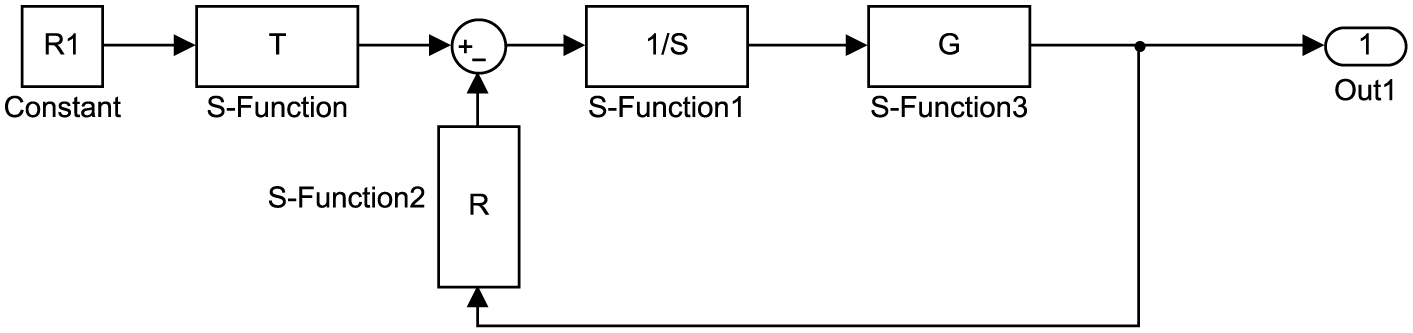
The controller output U is a function of both the error E and plant output C. Since the error, input and output are related by $E = R_{1} - C$ , there are other ways of setting this structure up to form a control signal U which is a function of any two of the three variables E, R₁ and C. It is often given the name ‘two degree of freedom control’, and some readers may be more familiar with the structure which uses a feedforward from the reference input. A more general description, often given in more advanced textbooks³ which discuss pole placement, is shown in Figure 2 where T, S and R are polynomials in s. It is easy to show that Figures 1 and 2 have the same closed-loop transfer function if $G_{c} = T / S$ and $F = (R - T) / S$ .

Figure 2.

Block diagram for a polynomial approach to pole placement

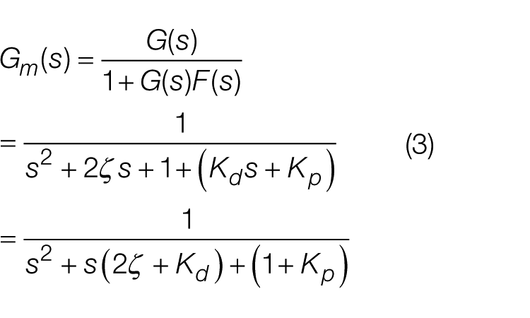
I prefer the structure shown in Figure 1 because it enables one to think of designing a proportional–integral (PI) controller for a modified plant G_m with a transfer function of

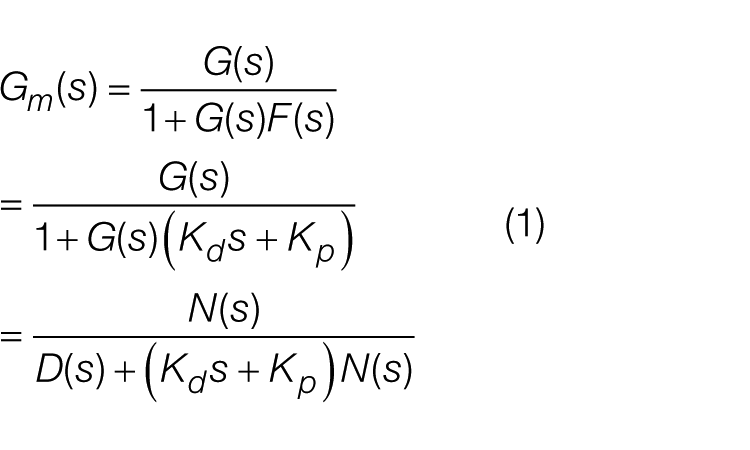
G_{m} (s) = \frac{G (s)}{1 + G (s) F (s)} = \frac{G (s)}{1 + G (s) (K_{d} s + K_{p})} = \frac{N (s)}{D (s) + (K_{d} s + K_{p}) N (s)}

(1)

when F is the PD transfer function $K_{p} + s K_{d}$ and $G (s) = N (s) / D (s)$ . This is a very useful concept if perhaps G has an unusual transfer function and a G_m can be found with a more ‘familiar form’.

Denoting the PI controller transfer function by $G_{c} (s) = (K_{1} s + K_{0}) / s$ and a PD with F, the closed-loop transfer function for the feedback loop of Figure 1 is

\frac{C}{R} = \frac{(K_{1} s + K_{0}) N (s)}{s D (s) + N (s) [K_{d} s^{2} + s (K_{1} + K_{p}) + K_{0}]}

(2)

The points to note about this transfer function are that the parameters of the PI controller affect both its poles and zeros, but those of the PD affect only the poles. Also, the increased complexity of the controller means one now has the difficulty of ‘tuning’ four parameters. Before discussing these aspects further, possible advantages of the structure are given:

(a) As mentioned previously, a ‘derivative kick’ is avoided.

(b) The response to a disturbance at the plant output is identical for PID and PI-D.

(c) There is only one zero in the closed-loop transfer function contributed by the controller. Although zeros do not affect the modes of a response, they do affect the magnitude of the contributions from each mode to the response. Thus, even if the closed-loop transfer function has all real poles, it does not guarantee, as with no zeros, that the closed-loop step response has no overshoot. The classical PID controller contributes two zeros to the closed-loop transfer function.

(d) The PD feedback changes the poles of the plant to be controlled by the PI from those of G to those of G_m. That is, it might be possible to change the plant to one which ‘is easier to control’ by a PI controller.

(e) The PD feedback may be regarded as a limited form of state feedback, that is, the feedback of two states, the output and its derivative. Theoretically higher orders of state feedback can be used to produce a suitable G_m. This topic is not considered further here, but the interested reader may refer to Atherton.⁴

III. Some Points about the Different Configurations

In order to bring out possible advantages of the controller configuration of Figure 1 , it is necessary to take examples with specific plant transfer functions.

A. Typical process plant

In the process control industry where PID controllers are tuned using Z-N concepts, there seems to be little gain apart from avoidance of the derivative kick in using PI-D rather than PID. Simulations for the two normalised plant transfer functions $G (s) = e^{- ρ s} / (1 + s)$ , for values of the time delay to time constant ratio ρ between 0.1 and 1, and $G (s) = 1 / {(1 + s)}^{6}$ show only small differences in the closed-loop step responses to set point changes if the results of the loop cycling method are used to tune the PID and PI-D controllers.

B. Position and speed control

PID controllers are used in these applications although the plant has an integrator in the case of position control. The first term is required to counteract disturbance torques, not to ensure a zero steady state error to a set point change, as is typical in process control applications. It is possible, as with a process control plant to use the Z-N loop cycling method, to identify the critical point, but since the plant dynamics are normally quite different, other ‘tuning’ rules other than the Z-N ones need to be developed for use.^5,6 To look at possible advantages of PI-D, one needs to take a typical plant model such as the time-scaled transfer function $G (s) = 1 / (s^{2} + 2 ζ s + 1)$ which with PD feedback gives

G_{m} (s) = \frac{G (s)}{1 + G (s) F (s)} = \frac{1}{s^{2} + 2 ζ s + 1 + (K_{d} s + K_{p})} = \frac{1}{s^{2} + s (2 ζ + K_{d}) + (1 + K_{p})}

(3)

Thus, it can be seen that the K_d term can be used to produce a modified plant with higher damping which simulation results show can be controlled by a PI controller to give a much improved closed-loop step response.

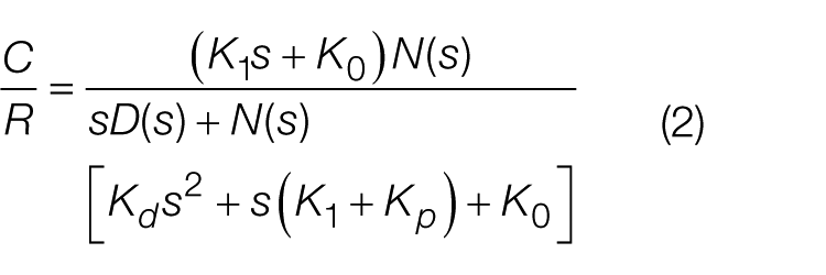
The closed-loop transfer function is

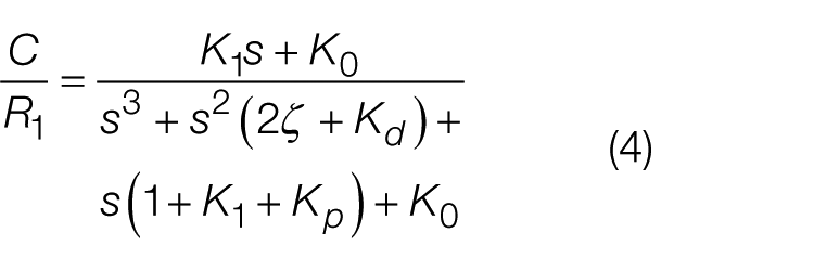
\frac{C}{R_{1}} = \frac{K_{1} s + K_{0}}{s^{3} + s^{2} (2 ζ + K_{d}) + s (1 + K_{1} + K_{p}) + K_{0}}

(4)

Boz and Atherton² look at the step response of transfer functions with a zero and show how the parameters can be chosen to produce suitable results, using the concept of standard forms of a transfer function.

C. Unstable plants

A simple example of an unstable plant transfer function would be the one used in the previous section with ζ zero or negative. It is clear from equation (3) that G_m can be made stable by a suitable choice of K_d. Another unstable transfer function K/(s² − λ) is often used as a model for control studies of a magnetically levitated body, and it is shown by Boz and Atherton² that this transfer function can be controlled in closed loop quite satisfactorily with PI-PD control. Unstable processes are sometimes modelled by a transfer function G(s) = Ke^−sτ/(1 − sT). This transfer function again can be controlled in closed loop with PI-PD control, which due to the time delay is not easily explained, so the interested reader is referred to Majhi and Atherton⁷ for further information. However, when there is no time delay, it is easily seen that again by writing down the expression for G_m, a suitable choice of K_d will makeG_m stable.

Regarding other situations, if a suitable low-order mathematical model with no zero can be found for the plant, then the approach of Boz and Atherton² mentioned at the end of section ‘Position and speed control’ can often be used to obtain satisfactory closed-loop performance. Obviously also, if suitable values for K_p and K_d can be chosen by some alternative method for a given G(s), then the loop cycling test can be used to select values for the parameters K₀ and K₁.

D. Pole placement

Many new theoretical approaches for looking at feedback control problems have been developed in recent years. They do have value where good mathematical models of the process to be controlled are available, but they have limitations in that (1) the theory can be difficult for the practicing engineer to understand; (2) the value, if any, relative to classical methods is not often clear; and (3) a user may have difficulty in understanding how to adjust parameters to improve performance ‘in situ’.

To illustrate these points, I have chosen an example from Corriou³ where controller designs are obtained using a pole placement based on the structure of Figure 2 . As mentioned in section ‘PI-PD Control’, R, T and S are polynomials in s and the plant transfer function taken in the example is $G (s) = 5 / (s^{2} + s - 2)$ , which is, of course, unstable.

The first solution given where no constraints are placed on the polynomials is $R = 0.2 s + 2.13$ , $S = s + 4.7$ and $T = 0.05 s + 0.25$ . It does give the closed-loop step response of $0.25 / (s^{2} + 0.7 s + 0.25)$ which is specified in the design approach, but why is there no steady state error with no integrator present? Simple, if you do the algebra, the desired closed-loop transfer function is obtained because $5 \times (2.13 - 0.25) = 2 \times 4.7$ , that is, the difference between the constant terms in R and T multiplied by the numerator of the plant transfer function is equal to the denominator plant coefficient of two times the constant term of S! Thus, errors in any of these values will mean a steady state error to a set point change. It is recognised that the approach is not good but not dismissed as unsuitable in practice, and the aforementioned simple explanation is not given.

The second solution given puts a constraint on the polynomial S, namely that s should be a factor, so that the error channel controller T/S will contain an integrator. One solution obtained, as many are possible using parameter choices which are difficult to relate to practical considerations normally of interest, such as response speed, gives $R = 9.22 s^{2} + 21.0 s + 5.39$ , $S = s^{3} + 7.30 s^{2} + 24.2 s$ and $T = s^{2} + 3.97 s + 5.39$ . I have given the numbers to three figures, not to five or six as done in the book, so perhaps it is not as easily noticed that the constant terms in both R and T are equal (given as 5.3852). For the configuration of Figure 1 , this gives $T / S = (s^{2} + 3.97 s + 5.39) / (s (s^{2} + 7.30 s + 24.2))$ and $F = (8.22 s^{2} + 17.1 s) / (s (s^{2} + 7.30 s + 24.2))$ . The s cancels in F due to the equal constant coefficients in R and T, so there is no integrator in F as one would expect.

The closed-loop response, to a unit step change in input at 1 s, for this design is shown in Figure 3 as curve 1. For further insight, a standard form design based on the integral square time error (ISTE) criterion was done with no time scaling for a PI-PD controller and a slight adjustment made to the coefficients to produce a similar response with negligible overshoot, which is shown as curve 2 on the same figure. 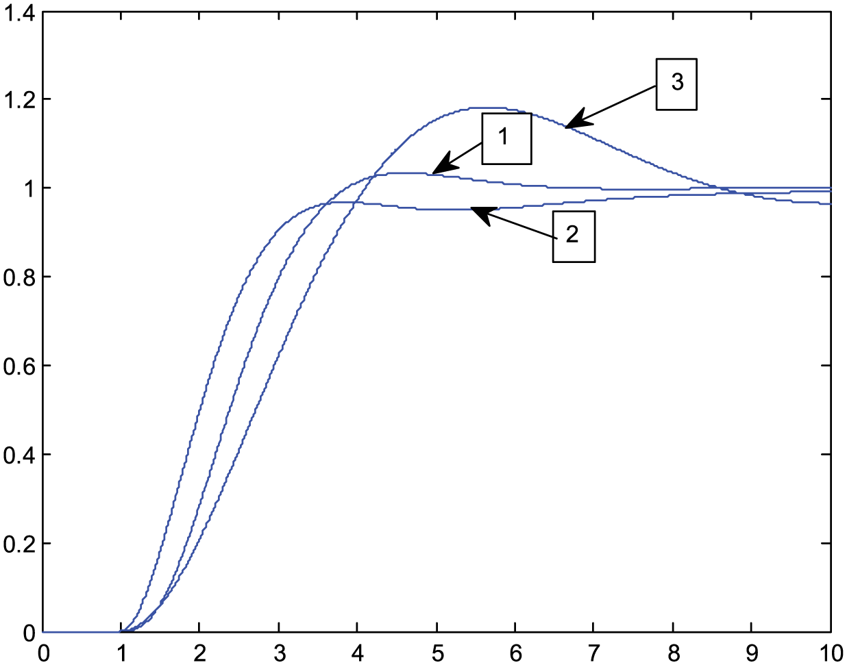The parameters of the PI-PD controller are $G_{c} (s) = (0.4 s + 0.2) / s$ and $F = (0.27 s + 0.66) / (1 + 0.002 s)$ with the derivative filter. Also shown, curve 3, is the step response for a PI-PD controller with the same F but $G_{c} (s) = (0.1 s + 0.2) / s$ . The parameters chosen here were obtained from an alternative frequency response fit to the G_c of the pole placement design. The Bode plots for these frequency responses are shown in Figure 4 again numbered 1–3. Figure 5 shows the Bode plots for the two F elements of the controller, the one labelled 1 being for the pole placement design.

Figure 3.

Step responses for different designs

Figure 4.

Bode plots for G_c

Figure 5.

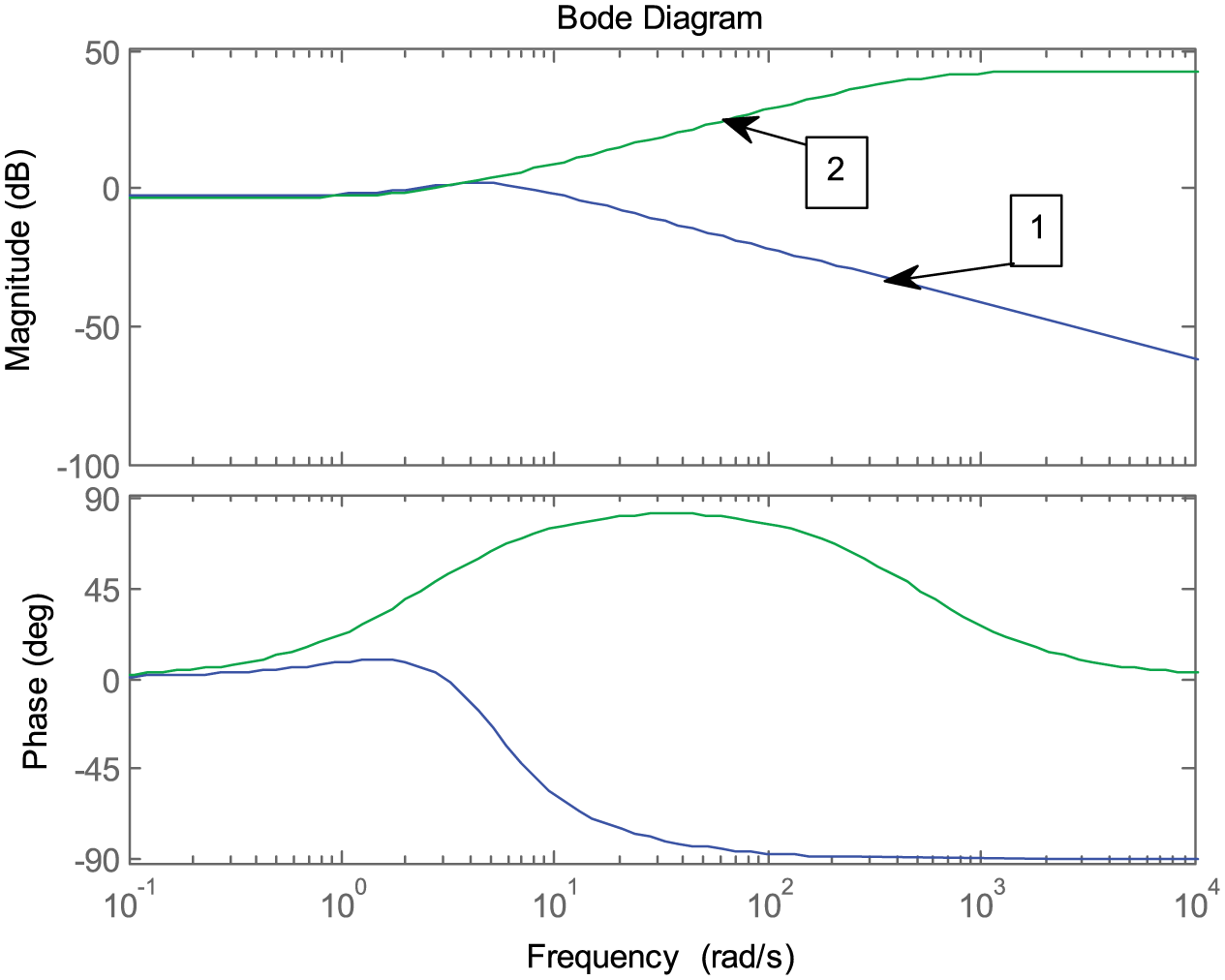
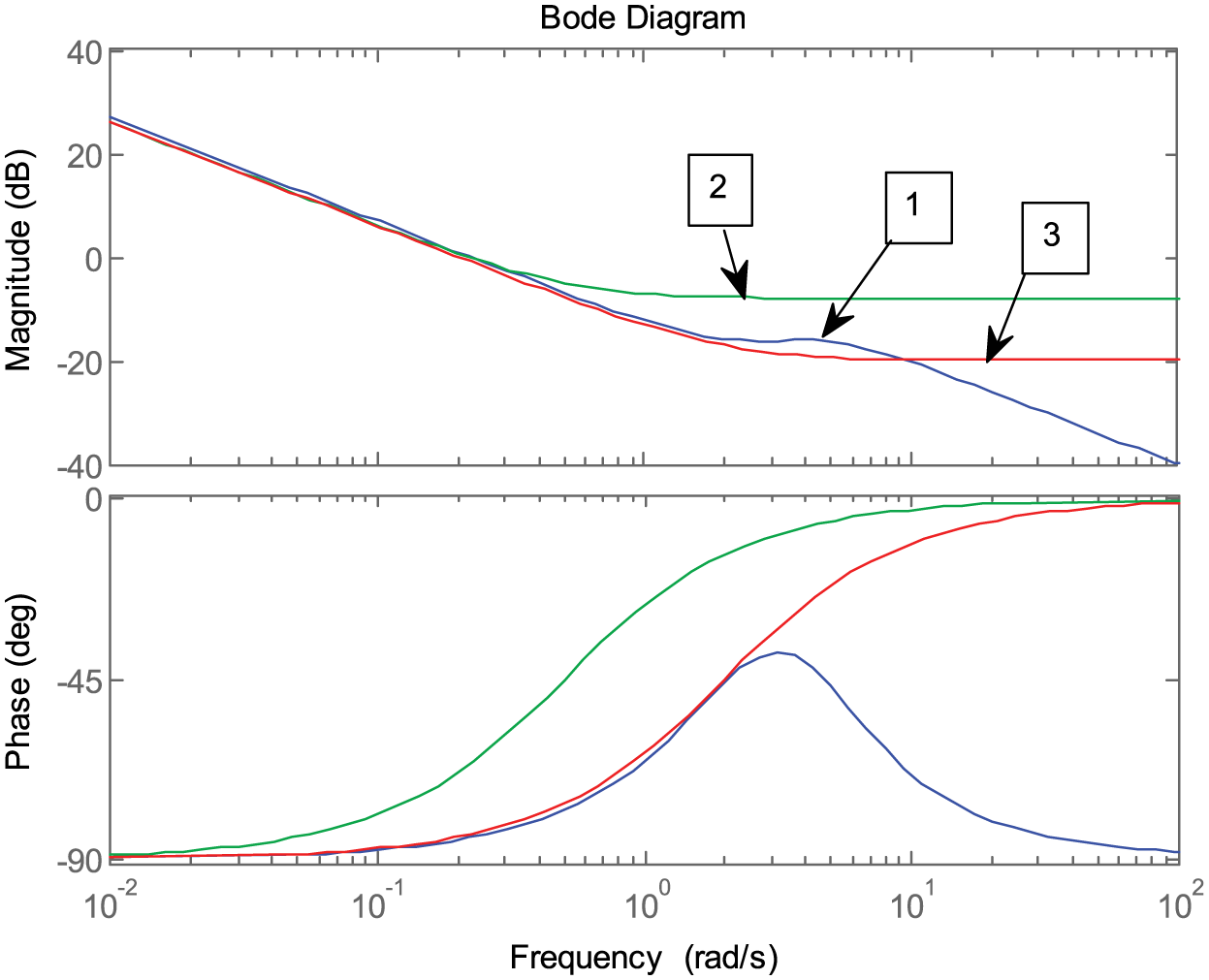
Bode plots for F

It can be seen from Figure 3 that the value of the proportional term in the PI term has not had a very significant effect on the step response. Also from Figure 5 , it is seen that the F term in the pole placement design shows an initial derivative action but with much lower bandwidth than the PD design. If for noise or other reasons it is desired to reduce the bandwidth of the PD term, then it is clear from the Bode plot how this can be achieved.

IV. Conclusion

I have tried to explain in this article by considering particularly the PI-PD version of the PID controller how plants with more ‘complex’ dynamics might be controlled by PID controllers. Many papers, particularly by academics, are published presenting new control ideas which fail to put the paper into context and use dubious methods for ‘proclaiming’ the advantage of their approach. Sometimes they compare their approach with PID control but in many cases fail to explain aspects such as the following:

The performance criteria to be addressed;

Whether their design and that used for the PID address the criteria directly or indirectly;

How they have obtained the parameters of the PID control (sometimes they do not even give them!).

From the material covered in section ‘Pole placement’, it is clear that the pole placement approach can give useful results, but I believe one should always look deeper into the significance of any results obtained. Furthermore, one should ask whether the results can be simplified by further ‘classical’ considerations and also look for the best practical implementation. The way the numbers have turned out in the design considered in section ‘Pole placement’ seems to indicate that the structure of Figure 1 is better than Figure 2 . Sadly, theoreticians seem to have a dislike for approximating results since once this has been done, they can no longer claim that some original, possibly desirable, property of the theory exists. Modern software, such as MATLAB, however, now allows analysis and simulation results to be obtained in a short time and at a small cost to check out a design even doing Monte-Carlo simulations to look at the effect of variations in parameters. Many theoretical results which claim robustness in design are based on working in the s-domain, while typically a practical designer wants robustness in the time domain. Unfortunately, the link between the s-domain and t-domain is limited to a few properties. Given a transfer function G(s), for example, with a single variable zero and three fixed poles, one cannot say whether its step response will have an overshoot without going to the t-domain.

Footnotes

Funding

The author(s) received no financial support for the research, authorship and/or publication of this article.

References

Atherton

. Setting the parameters of proportional-integral-derivative controllers. Measurement and Control 2015; 48(9): 273–7.

Boz

Atherton

. Using standard forms for controller design. In: Proceedings of the UKACC international conference on control 1998 (Contror98), Swansea University, Swansea, 1–4 September 1998, pp. 1066–71. New York: IEEE.

Corriou

J-P

. Process Control: Theory and Applications (Section 4.9). London: Springer-Verlag, 2004.

Atherton

. Achieving standard form responses using state feedback. In: Proceedings of the ICC2006, Glasgow, 30 August–1 September 2006, paper no. 185, 5 pp. Glasgow: University of Strathclyde.

Boz

Atherton

. Phase margin design of phase lead controllers using autotuning. In: Proceedings of the IMACS symposium on mathematical modelling (2nd Mathmod), Vienna, 5–7 February 1997, pp. 787–92. Amsterdam, The Netherlands: Elsevier Science Publishers.

Atherton

Boz

. Autotuning of phase lead controllers. In: Proceedings of the 4th IFAC workshop on algorithms and architectures for real-time control (AARTC ‘97), Vilamoura, 9–11 April 1997, pp. 111–6. Oxford, UK: Pergamon Press.

Majhi

Atherton

. Online tuning of controllers for an unstable FOPDT process. IEE Proceedings: Control Theory and Applications 2000; 147(4): 421–7.

PI-PD,an Extension of Proportional–Integral–Derivative Control

Abstract

I. Introduction

II. PI-PD Control

III. Some Points about the Different Configurations

A. Typical process plant

B. Position and speed control

C. Unstable plants

D. Pole placement

IV. Conclusion

Footnotes

Funding

References