Research on Internal Flow and Performance of Swirlmeter with Different Swirler Cone Angle

Abstract

The performance of a swirlmeter (or vortex precession flowmeter) was numerically and experimentally evaluated. With methods from computational fluid dynamics, the flow fields of the swirlmeter were analyzed, revealing their flow characteristics. To obtain detailed flow information with the Re-Normalization Group k – ε turbulence model and SIMPLE arithmetic, which couples pressure and velocity, the three-dimensional unsteady incompressible flow of a swirlmeter was numerically simulated. By varying the cone angle of the swirler, the performance of the swirlmeter was analyzed. The results show that the pressure fluctuation frequency inside has a linear response to flow rate, and the swirlmeter achieves high accuracy over a large measurement range. The pressure fluctuation near the region between throat and diffusor was stronger than other regions offering then an ideal location to mount the piezoelectric sensors. Different swirler cone angles were shown to influence both pressure drop and fluctuation; smaller cone angles produced higher frequency fluctuations but larger pressure loss.

I. Introduction

A swirlmeter is a type of fluid oscillating flowmeter that has been widely used in the natural gas industry because of its high accuracy and large range of measurement. There are no moving parts, and therefore, it has high reliability and is also easy to install.^1,2

As in previous studies on the swirlmeter, experimental tests are the main method of analysis. ³ Dijstelbergen ⁴ elaborated on its operating principle and conducted experimental tests on the swirlmeter. The results obtained were that the output of the meter was linear and independent of viscosity and density. From an analysis of the results based on high-speed photography, De-Tao et al. ⁵ proposed and prototyped a more complete and concrete physical mode for swirlmeter fluid flow. Moreover, the helical angle of the swirler played a dominant role in the flow. Kay Heinrichs proposed a new method for signal detection that used two diametrically opposed pressure ports which produced two signals of equal amplitude but 180° out of phase. With differential sensors, this method increased the measuring range. ⁶ In experiments studying the fluid oscillation characteristics of a 50-mm-diameter swirlmeter in oscillatory and steady flows, Peng et al. ⁷ pointed out that energy dissipation in the fluid could attenuate the vortex precession and reduce the lower limit of the swirlmeter.

In recent years, computational fluid dynamics (CFD) simulations have been used to investigate details of the flow characteristics inside the swirlmeter. With large eddy simulation, Fu and colleagues^8–10 numerically investigated vortex precession and hydrodynamic mechanisms for the oscillations inside the swirlmeter. Using numerical simulations, Wu ¹¹ produced optimal designs of the swirler increasing the blade number from 6 to 7 and, by reducing the incidence angle, decreased both the lower limit and pressure loss. Cui et al. ¹² numerically studied the incident angle of the swirler on the internal flow and performance of the swirlmeter and found that a larger incident angle generated larger pressure losses.

Numerical studies, especially using CFD methods, on this kind of flowmeter are scant. This paper describes our numerical study of the swirlmeter. Details of its flow field are produced and its performance compared with actual swirlers having different cone angles is evaluated. For this purpose, experiments were performed and are described as follows.

II. Research Model

A swirlmeter of 50-mm diameter is numerically and experimentally studied. The main parameters of the swirlmeter are set as follows: pipe diameter D = 50 mm, throat diameter d = 32 mm, length of swirlmeter L = 230 mm and cone angle of swirler α (see Figure 1 for definition), which is set to 11°, 20° or 30°. The swirler is the most important component and the focus of analysis is on varying its cone angle.

Figure 1.

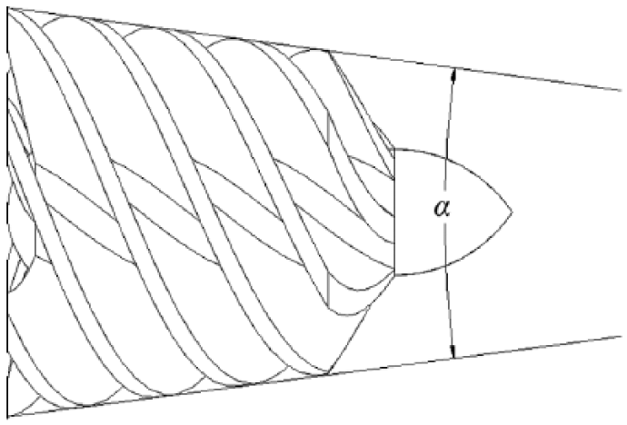
The sketch map of the cone angle α

The required assembly length of the straight pipe at the inlet and outlet of the swirlmeter was 3D and 1D, respectively. For the calculation, the extension length is set at 5D and 3D at the inlet and outlet, thereby meeting the required length.

III. Numerical Method

The calculation meshes were generated using the commercial software Gambit. In the region of the swirler, unstructured tetrahedron meshes were used for their great adaptability. For other flow regions, high-quality structured meshes were used to accelerate convergence. The total mesh number was about 1.6 million, this total being slightly different depending on the different models used. The surface meshes of the swirler and deswirler are shown in Figure 2 and the three-dimensional (3D) model of the swirlmeter and the computation domain are shown in Figure 3 .

Figure 2.

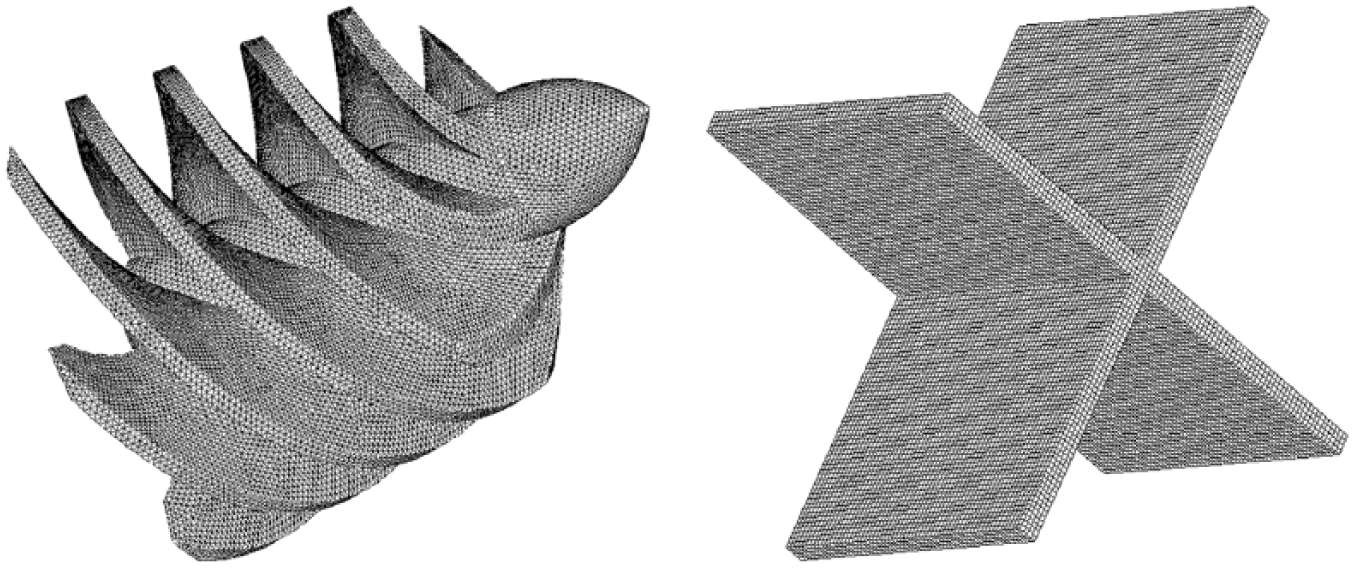
The surface mesh of swirler and deswirler

Figure 3.

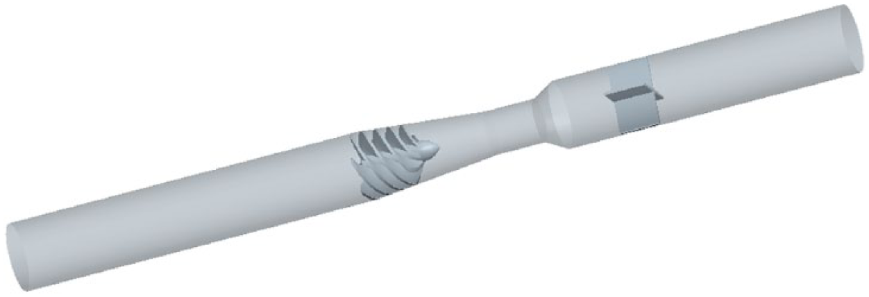
The 3D model of swirlmeter

For the numerical simulation, the Re-Normalization Group (RNG) k – ε turbulence model was used with SIMPLE arithmetic being applied to couple pressure and velocity. The inlet boundary condition involved setting the inlet velocity; the outflow boundary condition was selected at the swirlmeter outlet. In addition, a no-slip boundary condition and a standard wall function were adopted. A steady calculation result was set as the initial value for the unsteady simulation. To obtain the frequency of the pressure fluctuation at various monitoring points, the computational time interval was set to assure there would be at least 50 time steps for each fluctuation cycle. The flow rates were set from 6 to 100 m³/h at six different settings (specifically 6, 15, 25, 40, 70, 100 m³/h). The maximum velocity in this calculation was about 21.22 m/s. Being much smaller than Mach 0.3 (about 102 m/s), the air is assumed therefore to be an incompressible fluid in this simulation. All calculations were accomplished using software Fluent.

IV. Results of Numerical Analysis of the Swirlmeter

A. Static pressure distribution and internal flow

From the flow field and the pressure distribution at the mid-section of the swirler ( Figure 4 ; Q = 40 m³/h, t = 0.03614 s), pressure decreases rapidly in the swirler region, and the energy is transported along with the fluid, which impacts the swirler blades resulting in a pressure drop.

Figure 4.

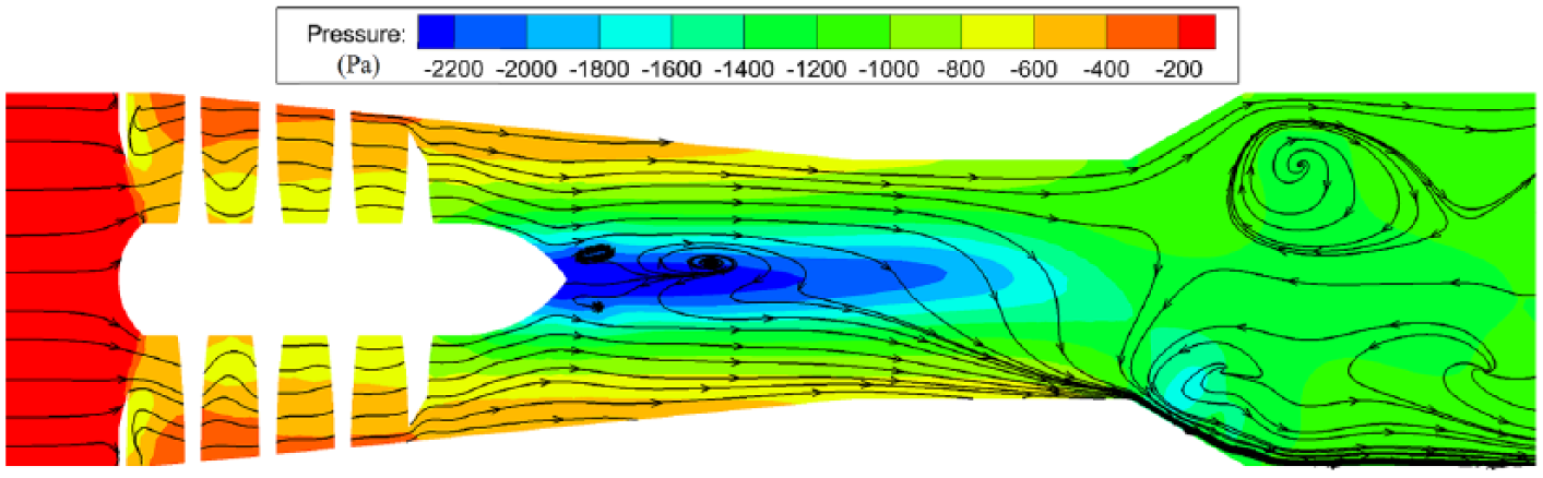
The pressure and flow field distribution at mid-section

The pressure decreases to a low level at the top of swirler cone (the outlet of the swirler), and the low-pressure area in the regions of convergence and throat (see Figure 5 for location) determines the core of vortex. Moreover, in these areas, the pressure distribution is essentially radially symmetric. Downstream of the throat, the vortex core is off-centered from the flow path due to the reflux at the end of the diffusor.

Figure 5.

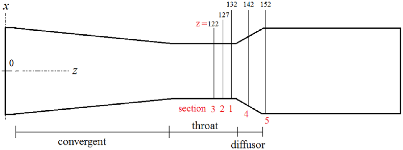
The 2D sketch map of the positions for different sections

B. Analysis of the pressure fluctuation characteristics

Pressure fluctuations were analyzed in different sections at the flow rate of Q = 6 m³/h, specifically because smaller flows produce weaker fluctuations. For greater flow rates, signal detection presents no problem; however, for slower flow-rate condition, strong fluctuations are required.

For the two-dimensional (2D) flow channel ( Figure 5 ), the flow state is found to be quite different from that in the throat and diffusor, and the pressure fluctuation near the junction region (z = 132 mm, denoted as Section 1) was the first to be analyzed.

The pressure fluctuations within Section 1 (Q = 6 m³/h) with different positions are shown in Figure 6 . The points are defined by coordinates (e.g. Point 132-6 refers to a z-coordinate of 132 mm and a x-coordinate of 6 mm). The pressure fluctuations are basically the same at different positions, the only difference being the intensity. Hence, for this case, intensity is the variable that needs to be taken into account.

Figure 6.

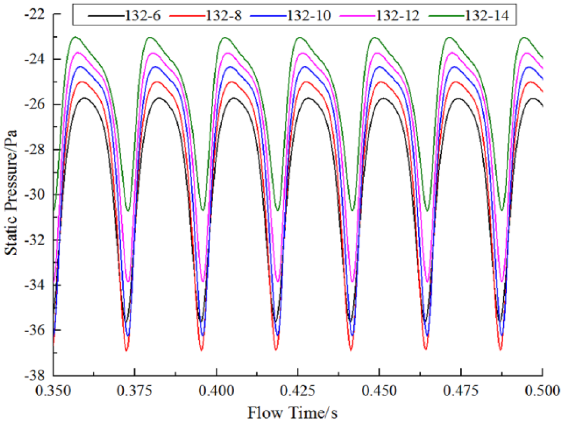
The static pressure fluctuation at section 1

For signal detection, stronger signals produce a larger range in pressure fluctuation. Nevertheless, as the piezoelectric sensor is positioned in the flow path, it therefore could disturb the intrinsic flow inside the flowmeter, particularly if the diameter of the flowmeter is as small as 25 mm or even only 50 mm. To reduce the effect of such disturbances and provide a clear detection of the signal, Point 132-10 positioned in Section 1 was selected. The sensor could then be assembled vertically inside with the working face being only about 6 mm away from the solid wall. The pressure fluctuations at a distance of about 6 mm from solid wall are shown in Figure 7 for the different sections. The various points are the same as defined for Figure 6 .

Figure 7.

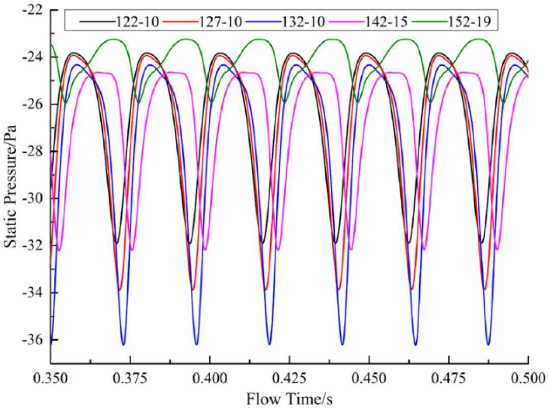
The static pressure fluctuation at different sections

From Figure 7 , the period of the fluctuation is the same for the different sections. This implies the pressure fluctuation frequency is independent of position and is not influenced by the location of data collection. The frequency of the fluctuation in the swirlmeter is used to determine flow rate.

Except for Section 5 (represented by Point 152-20), which is downstream of the diffusor, the fluctuations at other places are quite strong. Moreover, the solid wall at Section 4 is inclined and hence is unsuitable site for a sensor. The sensor should be mounted in the throat region (Sections 1, 2 and 3). Moreover, the pressure fluctuation at Point 132-10 is strongest indicating that signal detection within Section 1 might be better than other regions. Overall, taking the results from both Figures 6 and 7 into account, the best position for signal detection is at the end of the throat region with the sensor located about 6 mm deep within the flowmeter.

The pressure distribution (Q = 40 m³/h) in Section 1 over a fluctuation cycle is given in Figure 8 . The rotate of vortex at Section 1 is regular and indeed has the same dependence as for other positions. The only differences are in the magnitude for pressures and in the range for fluctuations. There exists a clear low-pressure area, which rotates anticlockwise with almost constant speed; its size remains steady with time. The motion of the periphery of the low-pressure area leads to the pressure fluctuating with a certain frequency at fixed positions. Because of the regular fluctuation, the piezoelectric sensor is able to detect a stable signal, which can then be converted to a flow rate.

Figure 8.

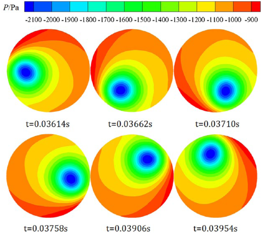
The static pressure distribution of section 1 in a cycle

C. Results’ analysis for different swirlers

In this section, the effect of different cone angle on swirlmeter internal flow field and performance are analyzed. Regarding the 3D models of three swirlers ( Figure 9 ), length, blade number and helical angle of each are the same; the only difference is the cone angle α being one of the settings 11°, 20° and 30°.

Figure 9.

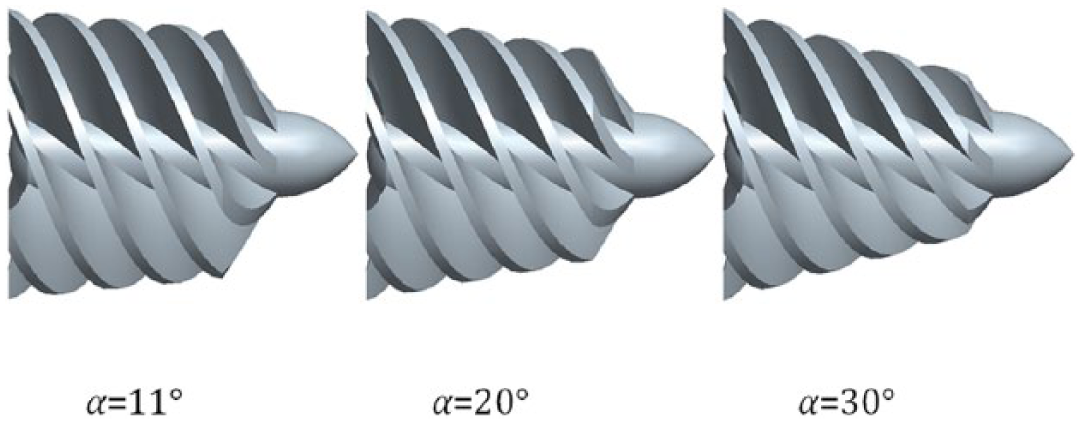
The swirlers with different cone angles

As the angle of convergence for the swirlmeter shell is 11°, there will be a gap for the 20° and 30° swirlers between swirler and swirlmeter shell. With an α of 11°, the air can only flow into the meter through the passages of the swirler, whereas for the other two swirlers, air will flow partially through the gap. Because the flow through the swirler region is changed, the generation of vortices is directly affected. As a consequence, the characteristics of pressure loss and pressure fluctuation frequency are different.

D. Analysis of fluctuation frequency

From the relationship between pressure fluctuation frequency f and flow rate Q ( Figure 10 ), frequency increases linearly with flow rate, at setting α = 11°. The linear relation is f = 9.0201 Q-6.508, with correlation coefficient of 0.9999, signifying therefore that the swirlmeter offers high accuracy over a large measurement range.

Figure 10.

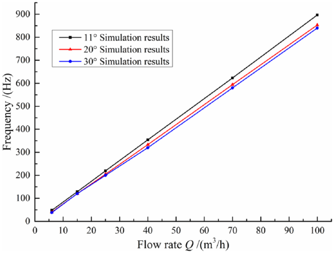
The fluctuation frequency for different swirlers

E. Analysis of pressure distribution for different swirlers

The static pressure distributions at the x = 0 cross section (Q = 6 m³/h) for the three swirlers ( Figure 11 ) show that the dependences are similar and therefore the cone angle of the swirler does not change the overall flow.

Figure 11.

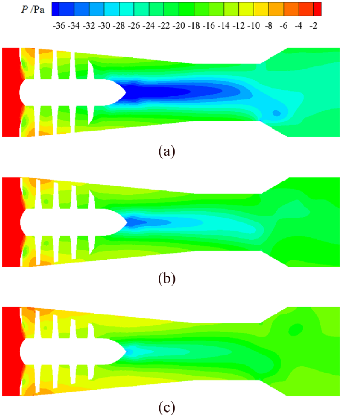
Pressure distribution at mid-section for different cone angles: (a) α = 11°, (b) α = 20° and (c) α = 30°

The variance of the pressure drop at the throat region is quite obvious. The largest cone angle produces the smallest pressure loss. For α = 11°, the pressure drops rapidly at the end of cone, and the energy loss is strong, whereas for α of 20° and 30°, these behaviors improve. For both, due to the gap between swirler and meter shell, the air flows either through the passages or through the gap. From the effect of the swirler passages, a vortex is generated with a specific intensity and speed. Because of the gap, air escapes, and this will decrease the intensity of the vortex. Both the pressure fluctuation frequency and pressure drop inside the swirlmeter are affected.

V. Analysis of Experimental Results

With a test rig (see Figure 12 ), experiments were performed using the sonic nozzle device chosen for its stable performance and high reliability. The actual model of the swirlmeter is depicted within the red rectangle of Figure 12 . The piezoelectric sensor registers the pressure fluctuation signal, which is converted to a pulse number to determine frequency f. The flow of the sonic nozzle is taken as the standard flow Q, from which the instrument coefficient K is obtained using equation K = f/Q. The pressure loss is obtained from the differential pressure transmitters, which process the pressure signal from the inlet and outlet of the swirlmeter.

Figure 12.

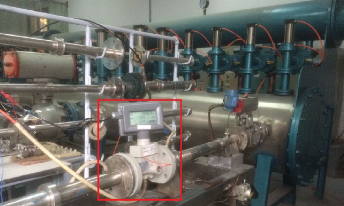
The test rig of the swirlmeter

From the pressure fluctuation frequency and the pressure loss ( Figures 13 and 14 ), all three swirlmeters produce strongly linear responses, although both frequency and pressure loss drop with increasing cone angle. With a larger cone angle, the surface of the swirler becomes smaller. Also, the effect of the blades working on the fluid diminishes resulting in weaker fluctuations and lower pressure loss. In such flowmeters, the pressure loss is significant, especially with large flow rates. For industrial use, swirlmeters with low pressure loss are required. Hence in choosing an appropriate cone angle, a balance between signal detection and energy loss is needed.

Figure 13.

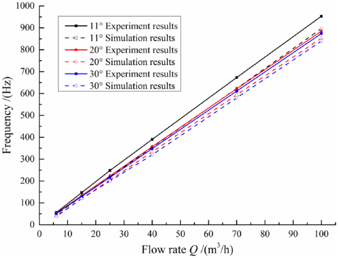
The pressure fluctuation results of simulation and experiment

Figure 14.

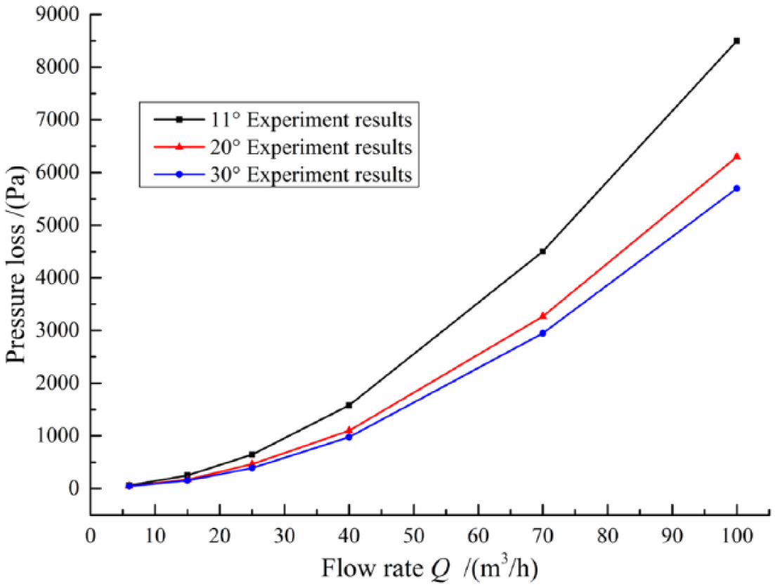
Experiment results of pressure loss for different swirlers

At large flow rates, the pressure loss is not negligible. From the experiment test, as cone angle increases from 11° to 20°, the pressure loss drops by about 10%, and this change enlarges the upper limit and widens the measurement range.

The trends from simulation and experimental results ( Figure 13 ) are roughly the same, the difference between them being about 5%. By increasing α, the fluctuation frequency and energy loss will be smaller. The fluctuation frequency drops along with pressure loss with increasing cone angle. With α = 30°, attenuating the vortex brings about a great improvement in pressure loss. However, with small flow rates, device performance is impaired and the lower limit increases. The 20° swirler yields the best results in this study as the lower limit is guaranteed; compared with the 11° swirler, the pressure loss decreases by over 10% at large flow rates.

VI. Conclusion

The performance of the swirlmeter was numerically evaluated. Employing CFD methods, flow fields of three swirlmeters with different cone angles were analyzed to determine their flow characteristics. These swirlers were studied to analyze the effect of cone angle on pressure loss and fluctuation frequency. Experimental tests were performed with the sonic nozzle standard device to verify the numerical results.

The analysis of the pressure fluctuation showed that the best position for the piezoelectric sensor was at the end of the throat. With stronger signal and less disturbance to the flow field disturbance, the sensor was best mounted at the end of the throat region at about a 6-mm depth inside the flowmeter.

The pressure fluctuation for different flow rates exhibited high regularity. Its frequency depended linearly on flow rate. The swirlmeter possessed high accuracy over a large measurement range.

The cone angle influenced both pressure loss and fluctuation frequency; a stronger fluctuation comes with a better signal but larger pressure loss. To choose an appropriate cone angle requires taking both these quantities into account. In this type of swirlmeter, a swirler with cone angle of 20° balances the performance, yielding reduced pressure loss over a large measurement range.