Setting the Parameters of Proportional–Integral–Derivative Controllers

Abstract

This note starts by discussing what is regarded as the pioneering work in proportional–integral–derivative controller tuning by Ziegler and Nichols. The basic concepts in their paper, rather than the specific tuning rules they presented, are held to be their major contributions. It is then explained with some brief theory how the ideas have been developed and how with modern technology the loop cycling method has been automated.

I. Introduction

Proportional–integral–derivative (PID) or three-term controllers are still extensively used in the process industries although their technical design is far different from their early use around 80 years ago (see Edwards and Otterson ¹ – Tech Talk for some basic material). For their use in a feedback control loop, the three parameters P, I and D need to be set to achieve a satisfactory performance, and the first major contribution to the topic was the study by Ziegler and Nichols. ² Ziegler and Nichols, often referred to as Z and N, worked for the Taylor Instrument Companies in the United States, the former being in the Sales Engineering Department and the latter in the Engineering Research Department. The paper is well worth reading not only for the contribution of Z and N but, since the paper was presented at the annual meeting of the ASME in New York City in December 1941, also for the discussion comprising around 30% of the total, to which four other industrialists contributed – a topic sadly missing from today’s publications.

To quote first from the abstract ‘These units form the basis of a quick method for adjusting a controller on the job’ and also from the introduction ‘The paper will thus first endeavour to answer the question: “How can the proper controller adjustments be quickly determined on any control application”’ No process mathematical models are introduced in the paper, so I believe the paper might have resulted from a conversation between Ziegler and Nichols which might have gone along the lines. Ziegler – when I visit plants where our controllers are being used, the users are often not happy with the system response, what simple procedure can I suggest to them to improve the situation? Nichols – let me think about that and do some experiments. The result is the paper which presents two suggestions after describing some experiments.

Unfortunately, not a great deal is stated about the process on which the experiments were performed. It is stated that

To simplify terminology we will take the most common type of control circuit in which a controller interprets the movement of its recording pen into a need for corrective action, and, by varying its output air pressure, repositions a diaphragm-operated valve.

P control is first discussed on what is then referred to as a ‘typical application’ which, apart from possible valve nonlinearity, is generally believed to have had a mathematical model near to that of first-order plus dead time (FOPDT). What would now be referred to as the ‘P’ gain is called ‘sensitivity’ and the ‘proportional band’ as ‘throttling range’. Pen recorder plots are given for both disturbance and load change responses as the sensitivity is changed, and the term amplitude ratio is used to refer to the relative magnitude of oscillations in the response, although it is not entirely clear whether it is overshoot to overshoot or overshoot to undershoot. An amplitude ratio of one is a continuous oscillation, and the sensitivity giving this is referred to as the ‘ultimate sensitivity $S_u$ ’, and the resulting period of oscillation is denoted $P_u$ . The trade-off between the sensitivity and the resulting responses and offset (steady-state error) is discussed. From these, they suggest a ‘good response’ (judged to be around 25% or 30% overshoot and not clear whether referring to disturbance or load change) is one with a sensitivity of $0.5S_u$ . Automatic reset, the introduction of the I term is then discussed with the first statement ‘Its only use is to eliminate off set’. Similar experiments are then carried out with PI control to suggest good parameter settings, with the term reset rate used for the inverse of the integral time constant and then repeated for PID, where the derivative time constant is referred to as pre-act. The process as expected was quite slow, so time constants were referred to in minutes. From the experiments, they suggested parameters, from measurements of $P_u$ and $S_u$ , which is now often known as the loop cycling method, as given in Table 1 .

Table 1.

Z-N method 1 parameters

Type	K	Ti	Td
P	0.5Su
PI	0.45Su	Pu/1.2
PID	0.6Su	Pu/2	Pu/8

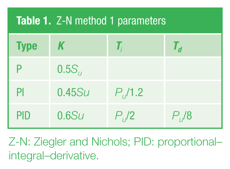
Z-N: Ziegler and Nichols; PID: proportional–integral–derivative.

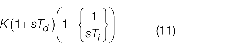
Here, K is the controller gain, T_i is the integral time constant and T_d is the derivative time constant, for an assumed ideal controller transfer function of

$$K\left(1+s_n{T}_d+\left[\frac{1}{s_n{T}_i}\right]\right)$$

(1)

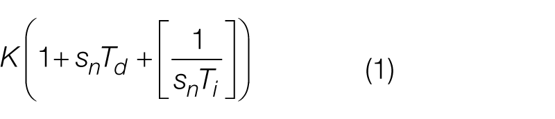
(Note that it is not entirely clear from the paper that this was the form of controller assumed to be fed by the error.)

The next step in the paper was to discuss how the parameters might be set from the ‘process reaction curve’, namely, from the step response of the process. They drew a ‘reaction curve’, which is defined as being approximately ‘S’ shape (bear in mind time cannot move backwards!). A tangent was then drawn to the curve at its maximum slope, which is designated, R, and the distance below the axis where this meets the time origin was denoted RL, so L is a delay measure for the response. From these experiments, the controller parameters of Table 2 were suggested.

Table 2.

Z-N method 2 parameters

Type	K	Ti	Td
P	1/RL
PI	0.9/RL	L/0.3
PID	1.2/RL	L/0.5	0.5L

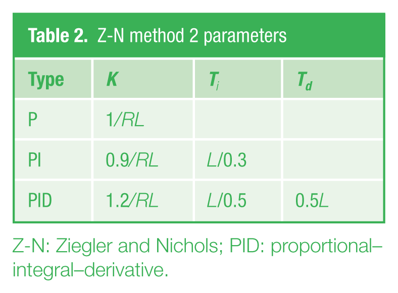
Z-N: Ziegler and Nichols; PID: proportional–integral–derivative.

Note that in the above two tables, the ratio of the gains in the first column and the time constants are consistent and that for the PID, the ratio of the integral to the derivative time constant is taken to be 4. Furthermore, for the rules to be identical requires (as mentioned by Z and N but taken no further) $L=P_u/4$ and $R=8/P_u{S}_u$ , which is clearly not the case for an FOPDT process as the period of oscillation with ultimate sensitivity is dependent on both the time constant and time delay, not just the latter as the first of the above expressions indicates. Furthermore, their ‘S’ curve does not correspond to a FOPDT process as the maximum slope for the FOPDT process occurs at the initial rise of the step response.

II. Relevance of the Z and N Paper

Viewed from today’s technology, one wonders why such imprecise results are still quoted. Although the wording is not used in the Z-N paper, they are today referred to as tuning rules, and they still provide the basis for ‘on the job’ controller settings. Both may be regarded as simple process ‘identification’ and then the setting of controller parameters based on the identification. The setting of the parameters is independent of the ‘identification’, and one could, therefore, use a different choice to Z-N.

The identification in the first approach, the loop cycling method, is of two process parameters namely, $S_u$ and $P_u$ , now often taken as the critical or ultimate gain, $K_c$ , and critical or ultimate frequency, ${\omega }_c$ , where the latter is normally taken in radians per second requiring time constants to be given in seconds, and Table 1 is given in many books in the form of Table 3 .

Table 3.

Z-N loop cycling method parameters

Type	K	Ti	Td
P	0.5Kc
PI	0.45Kc	0.8Tc
PID	0.6Kc	0.5Tc	0.125Tc

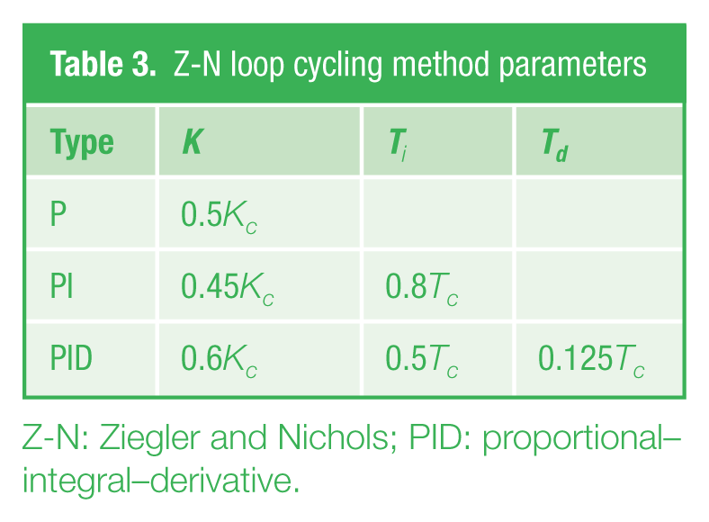
Z-N: Ziegler and Nichols; PID: proportional–integral–derivative.

Note that $T_i$ is often given in the PI controller as 0.8 not 0.833. The undoubted major contribution here of Z-N is to have recognised that from a simple closed-loop test on the plant, two parameters can be used to ‘identify’ it, namely, $K_c$ and ${\omega }_c$ , which are extremely useful for controller design. Assuming the plant is linear, these two parameters identify the frequency ${\omega }_c$ and gain 1/K_c where the phase is −180° on the Nyquist diagram, often referred to as the critical point for the process.

The second method, namely, obtaining the process step response to ‘identify’ it, was more familiar to control engineers at the time, and Z-N suggested one way of using this information. If the process model is taken as the FOPDT transfer function

$$G\left(s\right)=\frac{K_p{e}^{-s\tau }}{1+sT}$$

(2)

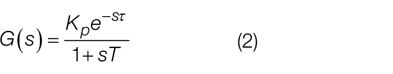
then it is easy to show that $R=K_p/T$ , which occurs at time, $\tau$ , and L = τ. Thus, direct substitution in Table 2 gives Table 4 , which is usually given in books.

Table 4.

Z-N method 2 based on FOPDT parameters

Type	K	Ti	Td
P	T/τKp
PI	0.9T/τKp	3.33τ
PID	1.2T/τKp	2τ	0.5τ

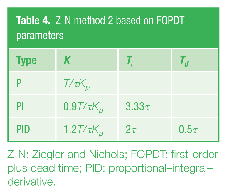
Z-N: Ziegler and Nichols; FOPDT: first-order plus dead time; PID: proportional–integral–derivative.

There are obviously various alternatives which might be used with this method in terms of fitting other models to the values in Table 2 or obtaining models, FOPDT or others, to fit a step response by alternative approaches. In practice, one has to obtain the step response of the process, which may not always be possible, and noise in the measurement may be a problem.

III. Time Scaling and the FOPDT Process

Since there are many other tuning algorithms given in the literature, ³ many of which are based on the assumption of an FOPDT process model, it is probably worth a slight digression here to discuss time scaling and the FOPDT process.

Amplitude and time scaling were very familiar to users of an analogue computer, where the latter was very useful according to the measurement device, for example, a slow plotting table or an oscilloscope. If for the FOPDT transfer function of equation (2), a normalised s, s_n, is taken equal to sT and with ρ = τ/T, then the transfer function becomes

$$G\left(s_n\right)=\frac{K_p{e}^{-s_n\rho }}{1+s_n}$$

(3)

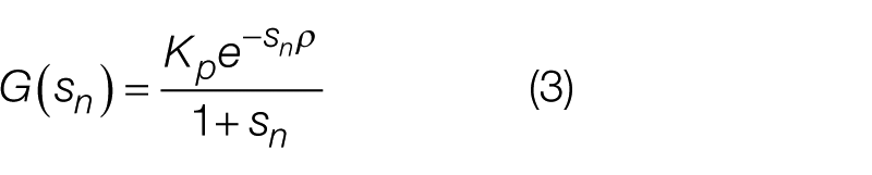
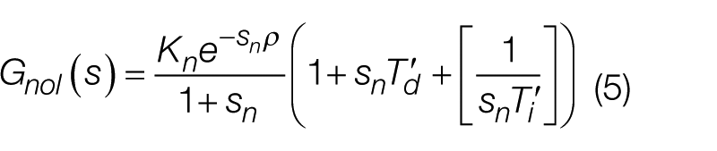
which can be referred to as a normalised FOPDT transfer function. The normalised transfer function has a unit time constant and only two parameters K_p and ρ. The actual system of equation (2) has a step response which is T times slower and markings on its frequency response T times smaller than that of equation (3). If this normalised plant is controlled by the ideal PID controller of equation (1) and fed with the error signal, then this becomes

$$K\left(1+s_n{T^{\prime }}_d+\left[\frac{1}{s_n{T^{\prime }}_i}\right]\right)$$

(4)

where ${T^{\prime }}_i=T_d/T$ and ${T^{\prime }}_i=T_i/T$ and the normalised open-loop transfer function can be written

$$G_{nol}\left(s\right)=\frac{K_n{e}^{-s_n\rho }}{1+s_n}\left(1+s_n{T^{\prime }}_d+\left[\frac{1}{s_n{T^{\prime }}_i}\right]\right)$$

(5)

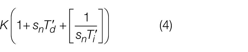
where Kn = K_pK. This means that if the controller parameters are designed based on some property of the open- or closed-loop transfer function, the results will be of the form

$$K_n=f_1\left(\rho \right),{T^{\prime }}_i=f_2\left(\rho \right)\mathrm{and}{T^{\prime }}_d=f_3\left(\rho \right)$$

(6)

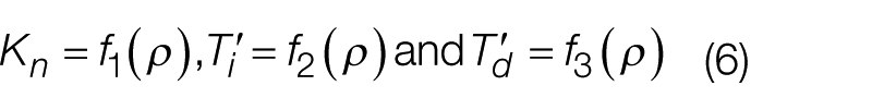
Thus, for any FOPDT plant, the controller parameters must be of the form

$$K=\frac{f_1\left(\rho \right)}{K_p},T_i=T{f}_2\left(\rho \right)\mathrm{and}{T}_d=T{f}_3\left(\rho \right)$$

(7)

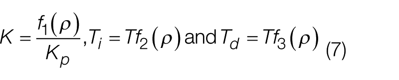
for the same performance property (i.e. time response) to be maintained for all FOPDT plants. This will be referred to as consistent tuning. Method 2 of Z-N is easily seen to be consistent with a simple choice for the functions f₁, f₂ and f₃ of being inversely proportional, proportional and proportional to ρ, respectively. It is also easy to show that method 1 is also consistent. Further discussion can be found on this topic in Atherton ⁴ but suffice to say here that not all the tuning algorithms given in O’Dwyer ³ are consistent.

IV. More on Loop Cycle Tuning and Critical Point Design

The loop cycling method has many desirable features, particularly the fact that the ‘identification’ is a closed-loop one, and the critical point provides useful information about the plant. Obviously, it is only applicable to processes where ${\omega }_c$ and $K_c$ have ‘reasonable values’, typically the case for processes with time delay but not for a process with a basically second-order mathematical model. It does, however, have several other practical problems. These include the following:

1. Even if the loop were linear, the fact that many processes have very long time constants makes it extremely difficult and time-consuming to try and find the gain, K_c;

2. It can be dangerous if there is no satisfactory limiting effect in the loop as an adjustment to an overestimated value of K_c can result in a large oscillation;

3. The oscillation may be quite noisy making obtaining good measurements possibly difficult or time-consuming;

4. Many practical loops are nonlinear. Saturation is helpful in limiting the amplitude of the oscillation, but dead zone effects may make finding K_c even more difficult.

With the advent of microprocessor controllers, Astrom and Hagglund, ⁵ possibly influenced by discussions with Mike Somerville the Technical Director of Eurotherm, suggested a much more suitable method of practical implementation for estimating the critical point. The method, which has become known as relay autotuning, involves replacing the P term by an ideal relay function to obtain a limit cycle. It can then easily be shown using describing function (DF) analysis ⁶ that the frequency of the limit cycle, ω_o, is approximately the critical frequency, ω_c, and the critical gain, K_c, is given approximately by K_c = 4h/aπ, where 2h is the peak-to-peak amplitude of the relay output, and a is the fundamental frequency amplitude of the limit cycle at the relay input. It can be shown that the estimate for ω _c will be better than for K_c and that the results will be better the nearer the limit cycle at the relay input is to a sinusoid. The error introduced by replacing a by half the peak-to-peak amplitude of the limit cycle, which is normally done in practice for ease of measurement, is usually quite small. The fact that the limit cycle amplitude can be controlled by the relay is useful in practice and also provides a mechanism for looking at the linearity of the process, provided time is available for repeated experiments.

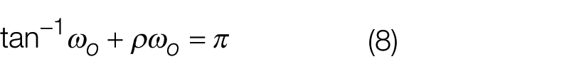
Thus, with a more practical approach for estimating the critical point, it is appropriate to comment further on the use of the critical point in PID tuning. First, what is the principle of the Z-N method 1 in using the critical point for tuning? Since all that is known about the plant is its critical point, then all one can do theoretically in selecting the controller parameters is to place this frequency at a known point on the compensated open-loop frequency response locus. To do this, one only has the freedom to vary two parameters, and in the Z-N method, this is done by taking T_i equal to 4T_d. This corresponds to the two zeros of the PID controller transfer function of equation (1) being real and equal. It is not entirely clear why this ratio of 4 for the two time constants was taken, although it seems to be a reasonable choice in many instances. My former colleague Mike Somerville, however, delighted in the fact that the two zeros being equal made sketching of the controller Bode diagram easy. It is easy to show that the point given by the Z and N tuning rules on the compensated locus is 0.5 arg − 180° for the P controller, 0.46 arg − 192° for the PI controller and 0.66 arg − 155° for the PID.

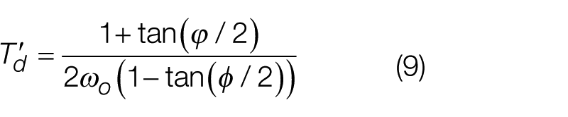
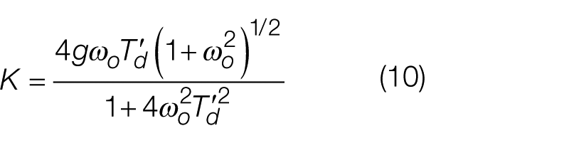
This concept is a useful design approach, and if felt appropriate, a different point can be chosen within the allowable range and an alternative to 4 can be selected for the time constant ratio. It is easy to show with T_i/T_d = 4, that is, for the FOPDT plant, the controller parameters are obtained from the following equations for moving the critical point to g arg − (180 − ϕ)°

$${\tan }^{-1}{\omega }_o+\rho {\omega }_o=\pi$$

(8)

$${T^{\prime }}_d=\frac{1+\tan \left(\phi /2\right)}{2{\omega }_o\left(1-\tan \left(\varphi /2\right)\right)}$$

(9)

$$K=\frac{4g{\omega }_o{T^{\prime }}_d{\left(1+{\omega }_o^2\right)}^{1/2}}{1+4{\omega }_o^2{T^{\prime }}_d^2}$$

(10)

Critical point design is a useful concept since closed-loop performance is very dependent on the open-loop frequency response in the region of the Nyquist critical point (−1, 0), as clearly recognised by Z and N. Certainly, if one has little knowledge of the plant dynamics, it can be very useful as illustrated here for a plant with transfer function G(s) and a possible reduced order model G_r(s), for which the step responses are shown in Figure 1 . The difference between the step responses is very small, and it would be difficult to detect with noisy measurements. However, the frequency responses shown in Figure 2 are quite different around the Nyquist critical point; indeed, G(s) has a finite gain margin while that of G_r(s) is infinite. Hence, a major problem in using step response data for design if one does not have some idea of the process dynamics (note the G(s) chosen was third order but not a typical process plant mathematical model ⁴ ). The major problem with a step response is that the higher frequency information is contained in the early part of the response, and variations may be difficult to detect in the presence of noise.

Figure 1.

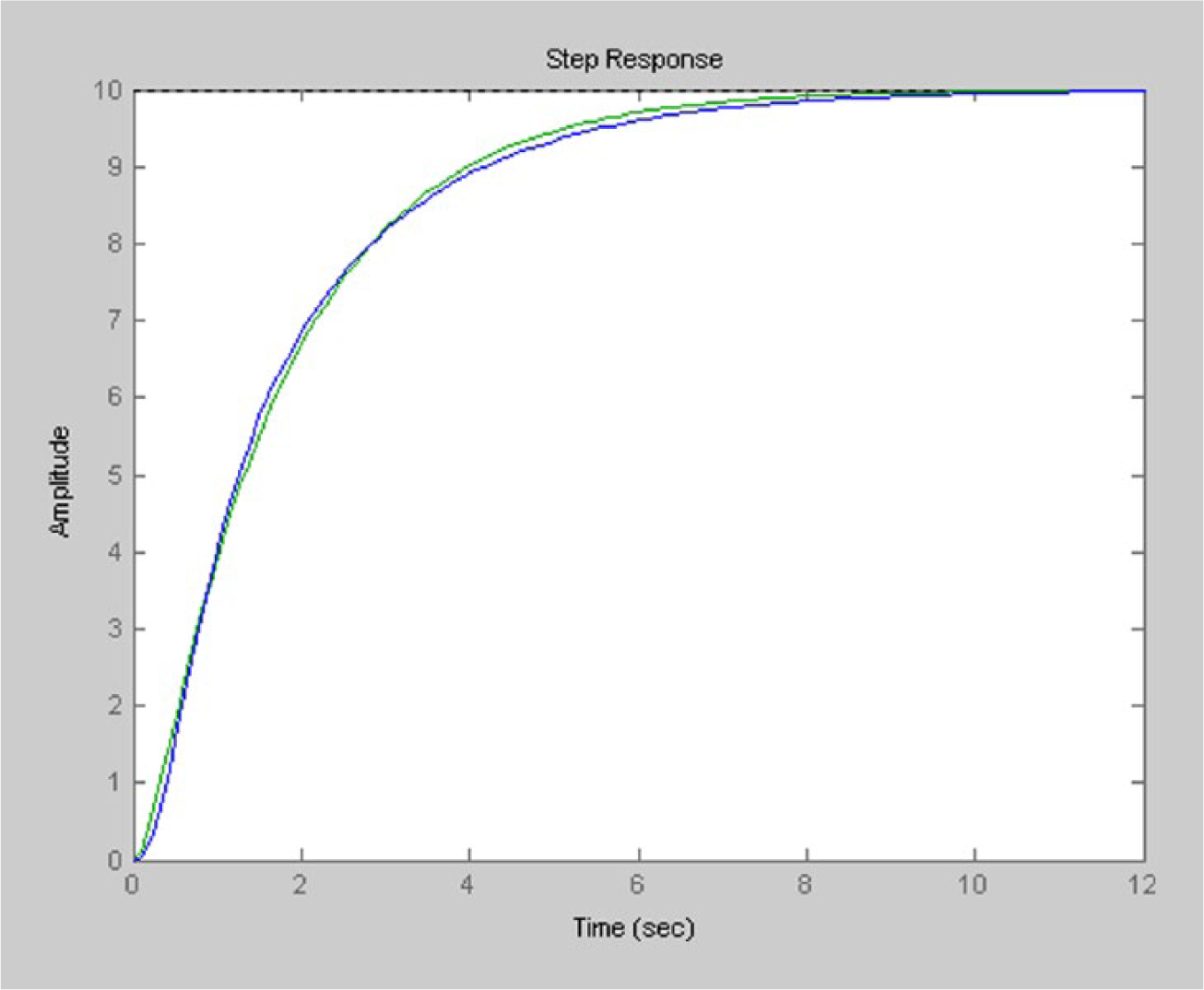
Step responses of G(s) and G_r(s)

Figure 2.

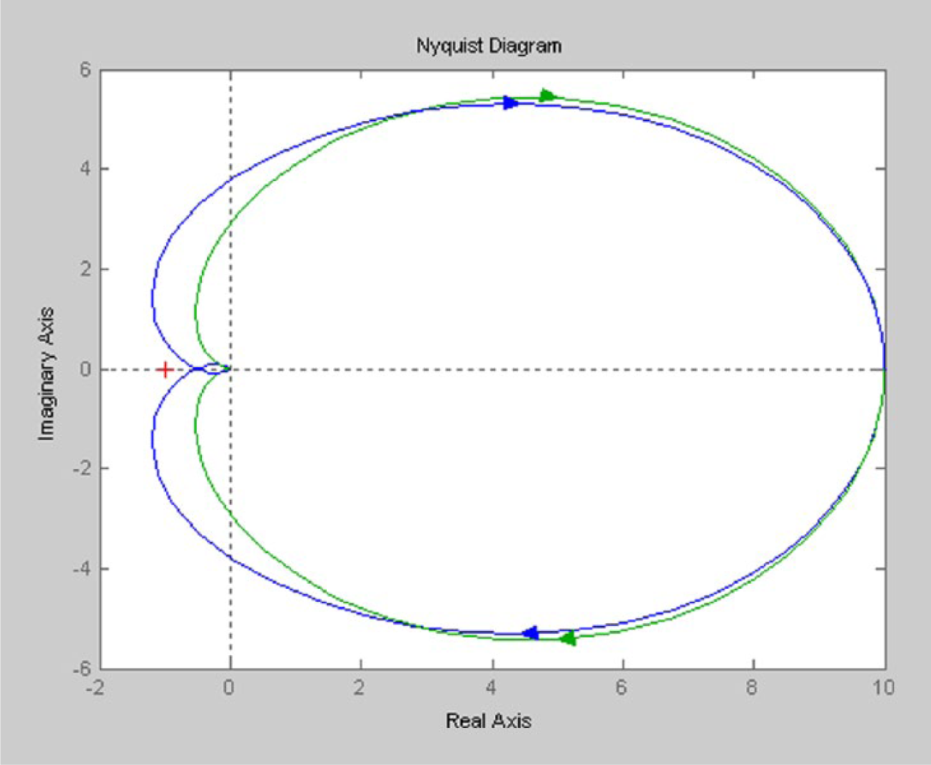
Frequency responses of G(s) and G_r(s)

Before concluding this section, it is probably worth mentioning that by including known networks in the loop with the relay, or using a relay with known hysteresis, additional information can be obtained on the process frequency response and/or more accurate measurements found. ⁶

V. Further Comments on PID Control

The number of papers and books written on PID control, mainly by academics, is huge, with many containing little of significance for the practising engineer. In practice, the ideal PID controller of equation (1) is never used, but its simple form allows ease of analysis and understanding. A pure D term is never used as theoretically it gives infinite gain at low frequency. It is normally replaced by $s{T}_d/(1+\alpha s{T}_d)$ with $\alpha$ typically less than 0.1. This term is also often fed from the process output rather than the error to avoid the ‘derivative kick’, since a step change in set point of, say r, produces a step change in error which if fed to $s{T}_d/(1+\alpha s{T}_d)$ ) gives an initial output of $r/\alpha$ . Even quite early controllers, certainly those in the analogue electronic days, as with modern controllers, were provided with integral wind-up protection. This is implemented in various ways with the sole purpose of stopping the integral term continuing to integrate when the input to the process reaches a saturation level. Other structures are also used where in addition to the PID of equation (1), the input is fed through a proportional term to the controller or the process output is fed through a proportional term. Another form of ideal PID controller sometimes used is

$$K\left(1+s{T}_d\right)\left(1+\left\{\frac{1}{s{T}_i}\right\}\right)$$

(11)

where a typical and easy design uses the derivative zero to ‘cancel’ a pole of the process.

The objective of selecting the PID parameters is to meet the specifications given for the control loop. These may, for example, be numerous, very simple or possibly difficult to translate into loop dynamic behaviour specifications. They might be easily met with many choices of parameters or very difficult to meet. They may refer to performance when regulating, typically with respect to disturbances or noise, or to changes in set point. With today’s microprocessor controllers, regulation parameters may be chosen differently from those for a set point change, and indeed, bearing in mind the Z and N statement regarding automatic reset, the integral term may be excluded except when near set point. Unlike other areas of control engineering, where typically it is expected that a good analytical designer can design a suitable controller using a mathematical model of the process with any one of many approaches, the PID field has become overburdened with so-called tuning rules. These are typically given whether the starting point is a mathematical model of the process or Z and N concepts, may be aimed at different specifications, which are often not clear, often compared inappropriately, and with dubious benefits. On the technical side, many controllers have one of several possible autotuning algorithms. Often they assume a model of a specific form for the process, so the manufacturer should be consulted before use on other than suggested processes.

VI. Concluding Comments

The purpose of this note has been to explain the valuable concepts in the early work of Z and N on PID tuning. Their formulae are regularly quoted but rarely is attention drawn to the simple experimental work with its imprecise details in terms of today’s technology. The contribution, however, is rightly regarded as very significant for the concept of the loop cycling method and the information it can yield and also for obtaining a possible mathematical model from simple tests on the process. This latter concept has now grown in control engineering into the huge field of identification.