Sage Journals: Discover world-class research

Abstract

In order to effectively recognize the rotating machine fault, a new method based on locality preserving projection and back propagation neural network–support vector machine model is proposed. First, the gathered vibration signals are decomposed by the empirical mode decomposition, and the corresponding intrinsic mode functions are obtained. Then, Shannon entropies of the intrinsic mode functions are used as the original features. But the extracted features have the problems of high dimension and redundancy. So, the manifold learning algorithm locality preserving projection is introduced to extract the characteristic features and reduce the dimension. The characteristic features are inputted to the back propagation neural network–support vector machine model to train and construct the fault diagnosis model, and the rotating machine fault condition identification is realized. The running states of a normal inner race and several inner races with different degrees of fault were recognized; the results validate the effectiveness of the proposed algorithm.

I. Introduction

Rotating machine is widely used in modern enterprise. Those rotating machines are often subjected to high loading and severe conditions during operation. Under this severe operating condition, defects are often developed gradually on the equipments. If no effective actions are taken, the failures of rotating machines can cause production breakdown and economical loss. Therefore, it is of prime importance to recognize the rotating machine state.¹

In order to achieve the rotating machine fault diagnosis, vibration signal feature extraction and intelligent state classification are the two most important aspects. For the former aspect, it mainly includes three categories: time domain, frequency domain and time–frequency domain analysis. Wavelet transform is the most commonly used time–frequency analysis method and is widely used in feature extraction. However, due to the factors such as clearances and nonlinear stiffness of rolling elements, vibration of a rotating machine, especially when faults have occurred, is essentially governed by a nonlinear dynamic model. For this reason, commonly used signal processing techniques aimed particularly for linear vibration signals including time and frequency domain techniques, as well as wavelet transform may all exhibit limitations. So it is necessary to find an effective method to extract the fault-related features hidden in the complex and nonlinear bearing vibration signals. Zheng et al.² proposed the use of the Shannon entropy and the wavelet to extract the features, and got a very good effect. However, some experiments show that there may exist energy leakage and aliasing between the adjacent scales of wavelet decomposition.³ Therefore, the empirical mode decomposition (EMD) method is used in this paper, and the EMD and Shannon entropy are chosen to extract the character features.⁴

As the features are extracted, however, the features still have high dimension and redundancy. In order to reduce the dimension of the features, some methods are proposed. Like linear embedding method principal component analysis (PCA), nonlinear locality-based learning methods, represented by locally linear embedding (LLE),⁵ Laplacian eigenmap,⁶ and Isomap⁷ that seek to discover the nonlinear structure of the manifold existing the given data set. However, their nonlinear property makes them computationally expensive. Moreover, they yield mappings that are defined only on training data points and it is difficult to naturally evaluate the maps of the testing set. Recently, a novel linear dimensionality reduction algorithm, called locality preserving projections (LPP) was proposed.⁸ LPP is a linear projective map that arises by solving a variational problem that optimally preserves the intrinsic geometry structure of the data set in a low-dimensional space. The key difference between PCA and LPP is that PCA aims to discover the global structure of the Euclidean space, while LPP aims to discover the local structure of the manifold. In many situations, LPP is capable of recovering important aspects of the intrinsic linear or nonlinear manifold structure by preserving local structure. Because of its ability to discriminate directions with the local largest variance in a given data set, the suitability of LPP for reducing the features dimension and extracting the most useful features as inputs of the bearing running state recognition model is investigated in this paper.

Another important aspect for bearing running state recognition is to establish the reliable state recognition model based on the extracted features. The existing equipment running state recognition methods can be roughly classified into model-based (or physics-based modals) and data-driven methods.⁹ Data-driven methods, known as artificial intelligent approaches, are derived directly from routine condition monitoring data of the monitored system. The more prior the data are used for the training process, the more accurate the model obtained. Artificial Intelligent techniques have been increasingly applied to bearing running state recognition, among which the most widely used models are neural network and support vector machine (SVM). The neural network has the problem of being only suitable for uniform distribution of the sample and may converge to local values. The SVM is good at identifying and classifying than the neural network, but it has the problem of not being sensitive to nonlinear characteristics; in many real applications, the input data cannot be identified precisely.¹⁰ The back propagation neural network–support vector machine (BPNN-SVM) method is used for clustering data than each of the method,¹¹ the particle swarm optimization (PSO) method is used to select the optimal parameters of the SVM, in this paper, the BPNN-SVM is used to realize the bearing running state recognition.

The remainder of this paper is organized as follows. The EMD Shannon entropy and the manifold learning method LPP are used to extract the features in section “Feature Extraction.” The BPNN-SVM model is presented in section “The BPNN-SVM Model for Fault Diagnosis,” in which the proposed method is validated using real-world bearing vibration monitoring data. Finally, the conclusions are given in section “Validation.”

The flowchart of the proposed method is shown in Figure 1 .

Figure 1.

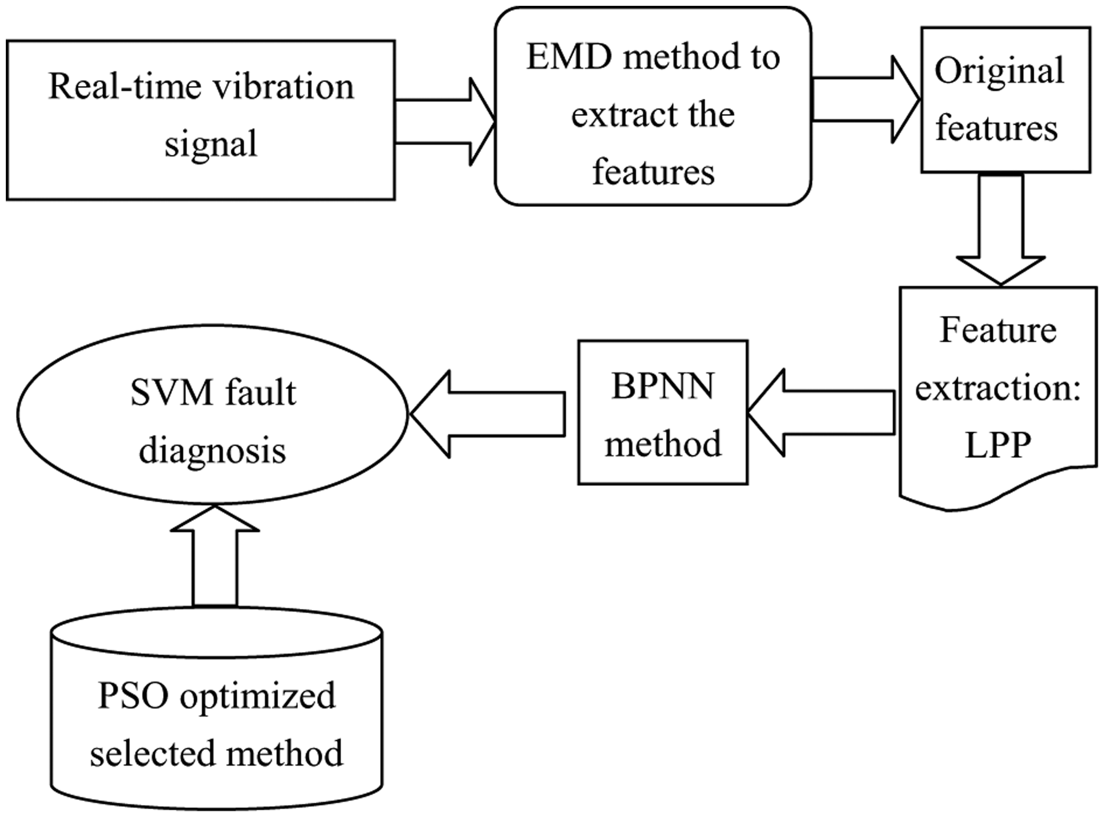
The flowchart of the proposed method

II. Feature Extraction

A. EMD energy entropy calculation

This section presents a brief discussion on feature extraction from EMD. EMD is developed to decompose a signal into intrinsic mode function (IMF) components and every IMF has a unique local frequency. The IMF should satisfy two conditions: (1) in the whole data set, the number of extreme and the number of zero crossings must either equal or differ at most by 1 and (2) at any point, the mean value of the upper envelope and lower envelope is zero.

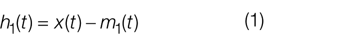
Once the extreme are identified, the maxima are connected by using the cubic spline and used as the upper envelope. The minima are interpolated as well to form the lower envelope. The upper and the lower envelopes should cover all the data in the time series. The mean of the upper and the lower envelope, m₁(t), is subtracted from the original signal to obtain the first component h₁ (t) of the sifting process

h_{1} (t) = x (t) - m_{1} (t)

(1)

Ideally, if h₁ (t) is an IMF, the sifting process will stop. So, it will shift the signal again in the same way to get another component h₂(t)

h_{2} (t) = h_{1} (t) - m_{2} (t)

(2)

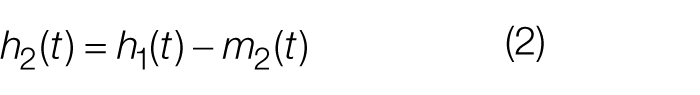
where m₂(t) is the mean of the upper and lower envelopes of h₁(t).

Repeat steps until the residual satisfies some stopping criterion. The signal can be expressed as

x (t) = \sum_{i = 1}^{n} c_{i} (t) + r_{n} (t)

(3)

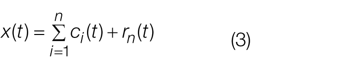
where n is the number of IMFs, r_n (t) is the residue which is a constant, a monotonic, or a function with only maxima and one minima from which no more IMF can be derived, and c_i (t) denotes IMF.

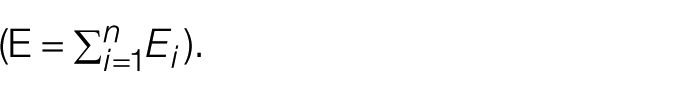
Once the n IMFs and a residue r_n (t) are obtained, where the energy of the n IMFs is E₁, E₂, …, E_n can be calculated respectively; then, due to the orthogonality of the EMD decomposition, the sum of the energy of the n IMFs should be equal to the total energy of the original signal when the residue r_n (t) is ignored. As the IMFs c₁ (t), c₂ (t), …, c_n (t) include different frequency components, E = {E₁, E₂, …, E_n} forms an energy distribution in the frequency domain of roller bearing vibration signal, and then the corresponding EMD energy entropy is designated as

H_{e n t r o p y} = - \sum^{n} p_{i} \log p_{i}

(4)

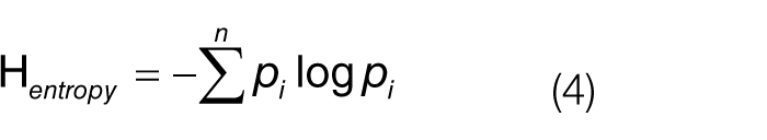
where p_i = E_i/E is the percent of the energy of c_i (t) in the whole signal energy

(E = \sum_{i = 1}^{n} E_{i})

B. The manifold learning method LPP

Manifold learning is a new unsupervised learning method. Its aim is to explore the intrinsic geometry information of data set, that is, to discover the inherent low-dimensional manifold embedded in the high-dimensional observation space. It has good performance to nonlinear reduction dimensionality.

In this section, the LPP is used to reduce the dimension and extract useful information. LPP aims to preserve the local structure of a data set. It seeks a transformation a to project high-dimensional input data X = [x₁, x₂, …, x_n] into a low-dimensional subspace Y = = [y₁, y₂, …, y_n]. A reasonable criterion for choosing a map is to minimize the following objective function

\min_{α} \sum_{i, j = 1}^{n} ‖ y_{i} - y_{j} ‖^{2} S (i, j)

(5)

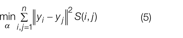
where y_i = a^Tx_i, and the weigh matrix S (called heat kernel) is constructed through the nearest-neighbor graph. The objective function with S incurs a heavy penalty if neighboring points x_i and x_j are close then x_i and x_j are close as well. In which the local structure of the input data can be preserved, specific algorithm description can be found in literature.⁸

III. The BPNN-SVM Model for Fault Diagnosis

A. The BPNN-SVM model

The BPNN model is a method that analog the decision-making process of the neurons in the human brain. The BPNN is commonly used in the pattern recognition. It is usually composed of three layers feed-forward network configuration, it works as an adaptive pattern recognition technique, and has a good adaptability and learning ability, but its recognition results easily fall into local minima problems. If it is used to achieve the machine fault diagnosis, the problem may cause the error. The SVM was first proposed by Cortes and Vapnik in 1995; it is based on statistical theory. The method achieves the machine learning under the conditions of small sample, nonlinear and high-dimensional pattern recognition. SVM achieve the optimization result based on the training error is the least, so is can ensure the global minimum. But the SVM pattern recognition result is easily affected by the input features and the parameters of the SVM, so the BPNN is used to first deal with the features to make the result that got by the SVM is more accurate. The parameters of the SVM are selected by the PSO method to get the parameters to match the SVM.

B. The SVM parameters’ selection

The PSO algorithm was used to select the SVM parameters. It is an optimization method based on a set of particles whose coordinates are potential solutions in the search space. Particles in PSO will change their coordinates (their solutions) by migrating. During migrating, each particle adjusts its own coordinates based on its own past experience and other particles’ past experiences.

The PSO was chosen to optimize the SVM parameters through the following formula

v_{i j} (t + 1) = w v_{i j} (t) + c_{1} r_{1 j} (p_{i j} (t) - x_{i j} (t)) + c_{2} r_{2 j} (p_{g_{j}} (t) - x_{i j} (t))

(6)

x_{i j} (t + 1) = x_{i j} (t) + v_{i j} (t + 1)

(7)

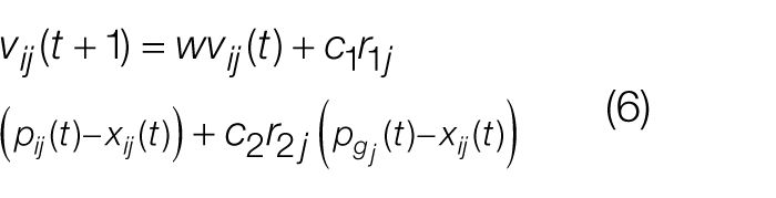
where the subscript “i” represents the ith particle and “j” represents the j-dimensional.

The subscript “t” represents the t generation. v_ij(t) is the velocity of the ith particle in the tth iteration, x_ij(t) is the position of the ith particle, p_ij(t) is the pbest position of the ith particle, and p_{g_j} is the gbest position (pbest represents the local optimum of the particles; gbest represents the overall situation optimum of the particles). The w represents the inertia weight. c₁, c₂ are learning factors. r₁ ∼ U(0,1), r₂ ∼ U(0,1) represent two independent random functions.

The process of optimizing the parameters γ, σ based on the PSO is given below:

At the beginning of the optimization process, randomly initialize population size, c₁, c₂, ω, rand(1), rand(2), determine the termination condition, positions and velocities of the particle, mapping the SVM parameters Υ, σ into a group of particles, and initialize the initial position of each particle, pbest, gbest of the particles;

When training the SVM, use equation (15) as the PSO fitness function;

Use the target parameters Υ, σ as the particles, use their initial values as the SVM parameters in step (2), and the corresponding value of equation (15) as the optimal solution of Υ, σ;

Use the initial error value of step (2) as the particle’s initial fitness value, search the optimal value as the global fitness value among the initial fitness value, and the corresponding particles as the current global optimal solution;

Update the velocity and position vector;

Re-substitute the updated parameters Υ, σ into the SVM model, and re-train the SVM model according to step (2), save the output value, and calculate the fitness value of the particles again;

Compare the saved global fitness value obtained in step (6) with the current particle’s fitness value; if the global fitness value is superior to the current particle’s fitness value, update the current particle’s fitness value according to step (5), and update the current particle’s optimal value equal to the corresponding particle’s optimal value obtained in step (6);

While the termination conditions are not met, return to step (5);

End loop.

IV. Validation

In order to verify the effectiveness of the proposed method, the proposed method is used on the actual application. The test rig is shown in Figure 2 .

Figure 2.

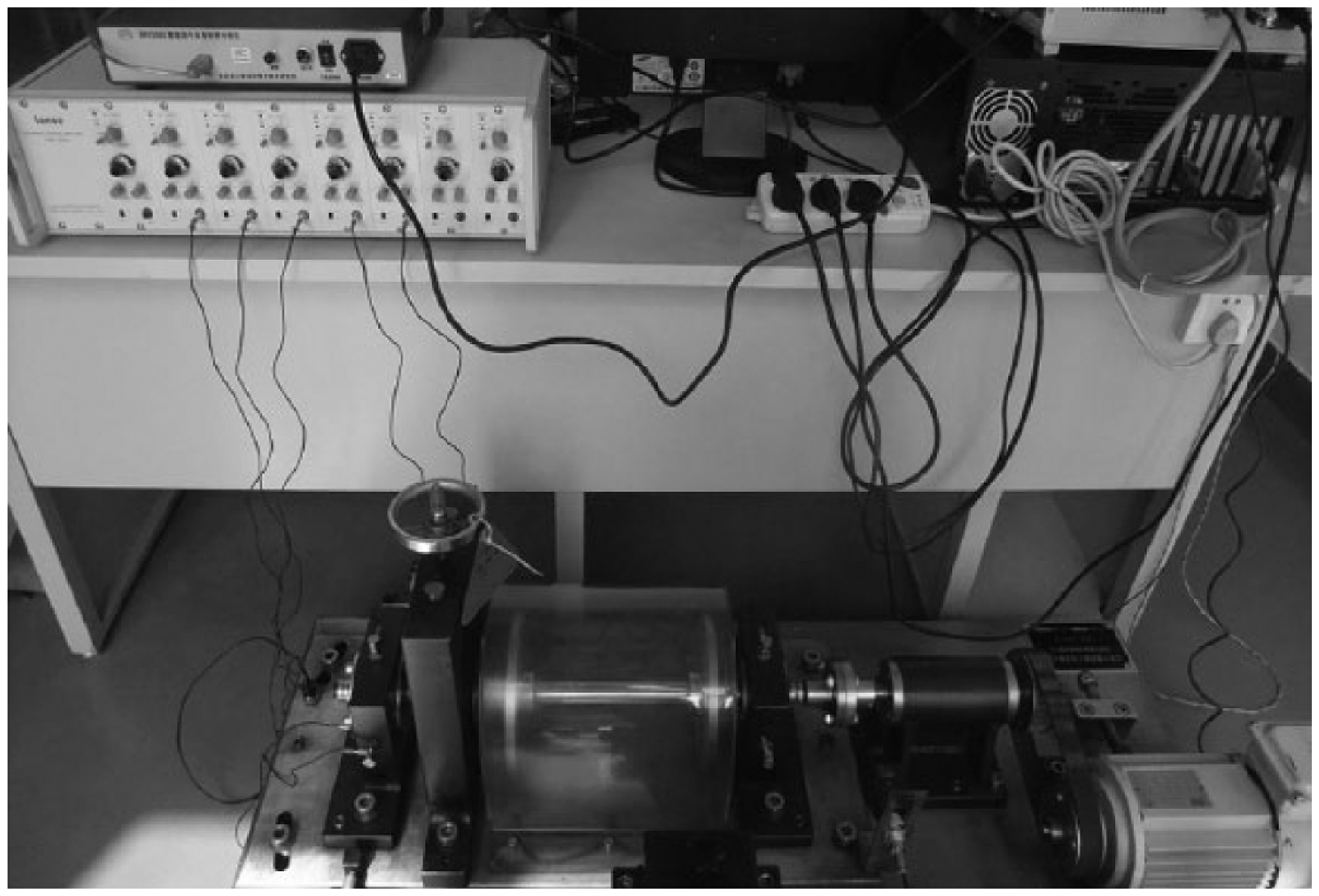
The test rig

The bearings are hosted on the shaft; the shaft is driven by AC motor. The rotation speed is kept at 1000 r/min. A radial load of 3 kg is added to the bearing. The data sampling rate is 25,600 Hz and the data length is 102,400 collected points, as shown in Figure 3 . Every 2 h, the vibration data are collected once. Then a set of data from each of the 2 months is selected; the data sets are used to test whether or not the proposed method can identify the bearing running state. A total of 4096 data points are selected for analysis, and 60 groups of collected data of different faults are obtained, with 30 groups for training and the other 30 groups for testing. The bearing has been running for 8 months, and because the amplitude of the bearing vibration exceeds the set threshold value, the bearing is considered invalid.

Figure 3.

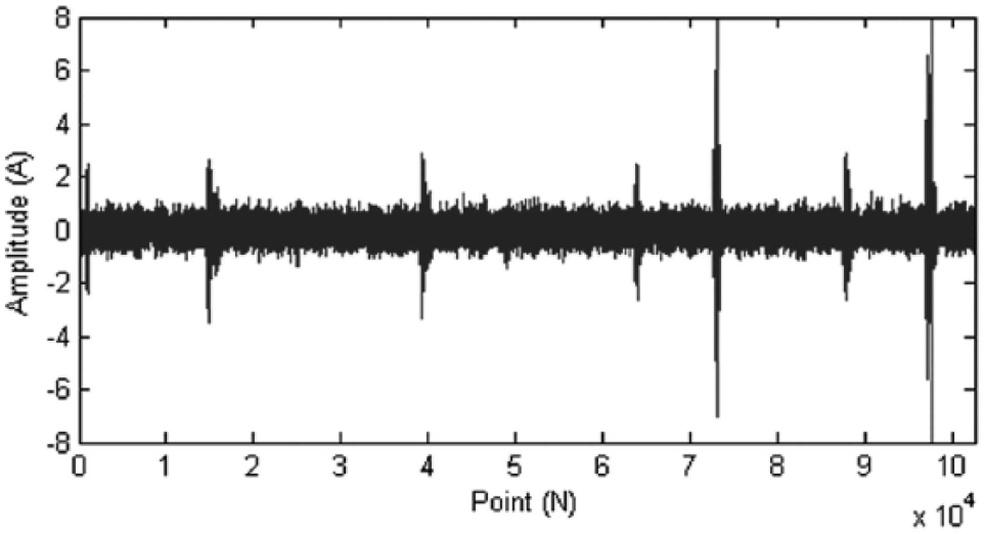
The collected vibration signal

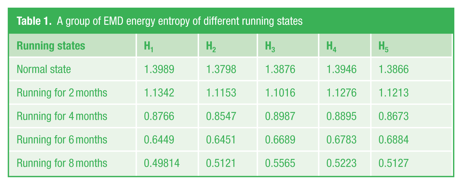
Next, the EMD decomposition was used to decompose each group of signals into IMFs, and Shannon entropy was used to extract the features. A group of EMD energy entropy (8 months) of Figure 3 is obtained, as shown in Table 1 (not normalized before).

Table 1.

A group of EMD energy entropy of different running states

Running states	H₁	H₂	H₃	H₄	H₅
Normal state	1.3989	1.3798	1.3876	1.3946	1.3866
Running for 2 months	1.1342	1.1153	1.1016	1.1276	1.1213
Running for 4 months	0.8766	0.8547	0.8987	0.8895	0.8673
Running for 6 months	0.6449	0.6451	0.6689	0.6783	0.6884
Running for 8 months	0.49814	0.5121	0.5565	0.5223	0.5127

Then, normalize the 20 groups of entropy values, and input them into the LPP to reduce the dimension. In order to compare the dimension reduction and redundant treatment effect of LPP, the manifold learning method Linear Local Tangent Space Alignment (LLTSA),¹² and the orthogonal locality preserving projections (OLPP)¹³ method are used to reduce the dimension. The results are shown in Figures 4 –6. To be comparable, the dimensions of LLTSA, OLPP and LPP are set to 3, so the input dimensions of the methods are set to 3 and the neighborhood number is set to 10.

Figure 4.

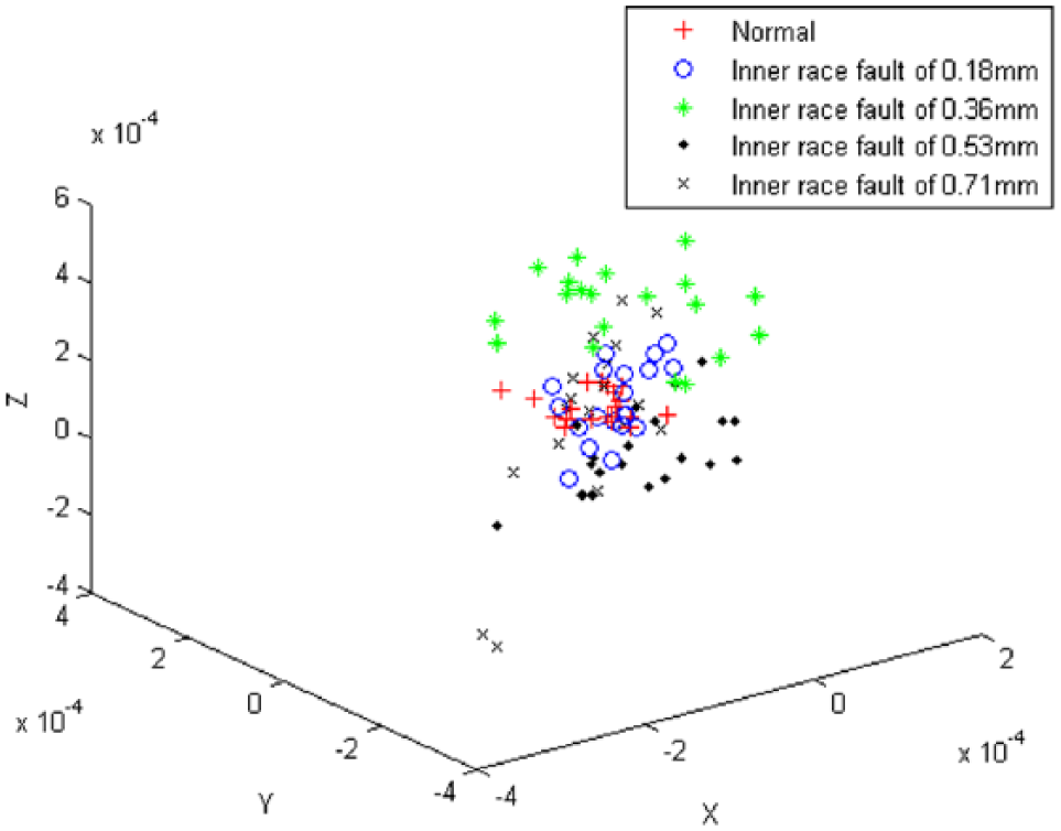
The dimension reduction and redundant treatment effect of LLTSA

Figure 5.

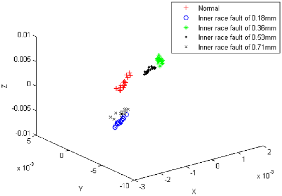
The dimension reduction and redundant treatment effect of OLPP

Figure 6.

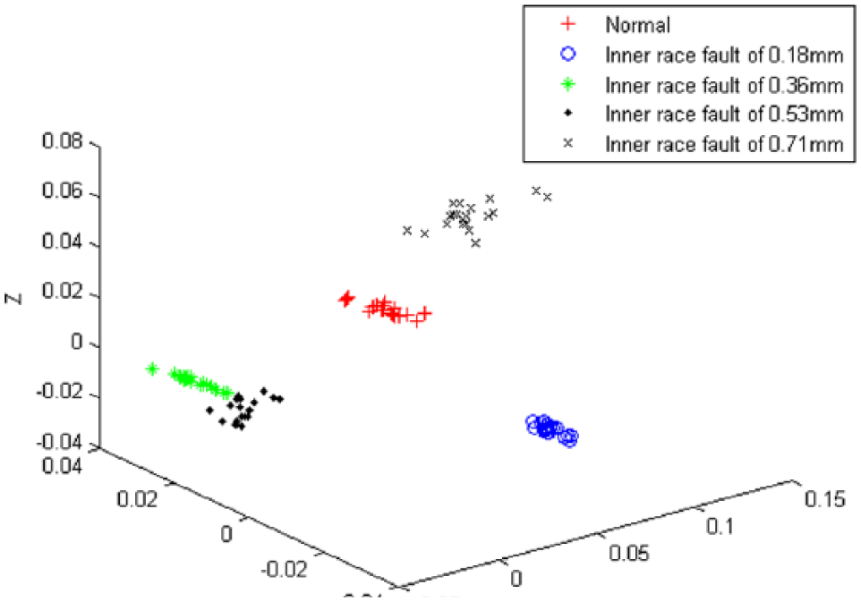
The dimension reduction and redundant treatment effect of LPP

By comparing the results of Figures 4 –6, the results show that the LLTSA-based data dimension reduction method cannot effectively separate the high dimension features, and there is still serious aliasing, which will affect the accuracy of the SVM state recognition effect. The OLPP-based data dimension reduction method works better than the LLTSA methods; however, they still have some data mixed together. The LPP-based data dimension reduction method can effectively separate the features of different running states with high calculation accuracy and a higher computational efficiency than the OLPP and LLTSA methods, which conforms more to the actual project requirement. Thus, in the study, the LPP method is selected.

After dimension reduction with the LPP, the extracted features are input into the BPNN-SVM to train the model so as to recognize the states. The learning rate of the BP neural network is set to 0.01; the iteration number is 2000; the training error is 0.0001; the hidden number n = 10; and the output number is set to 5. In order to verify the identification accuracy of the proposed method, the features extracted by LPP are input into the BP neural network, traditional radial basis function (RBF) SVM (with penalty factor C set to 100, nuclear parameter Υ set to 0.1), and the BPNN-SVM (the PSO is used to obtain the main parameters of the SVM model, the particle swarm population size is set to 100, and the number of the particles is set to 20. The fitness function is set to get the minimum prediction error with the optimized parameters. The prediction error is set to 0.0001. The PSO particle’s dimension is set to 2, the w is set to 0.5, the C1 is set to 1, and the C2 is set to 1) respectively. The comparison results are shown in Table 2 .

Table 2.

The recognition rate of traditional RBF SVM and the MWSVM

SVM type	Recognition rate η (%)
	Normal state	Running for 2 months	Running for 4 months	Running for 6 months	Running for 8 months
BP neural network	90	96	94	93	90
RBF kernel SVM	94	93	91	96	91
BPNN-SVM	100	100	100	100	100

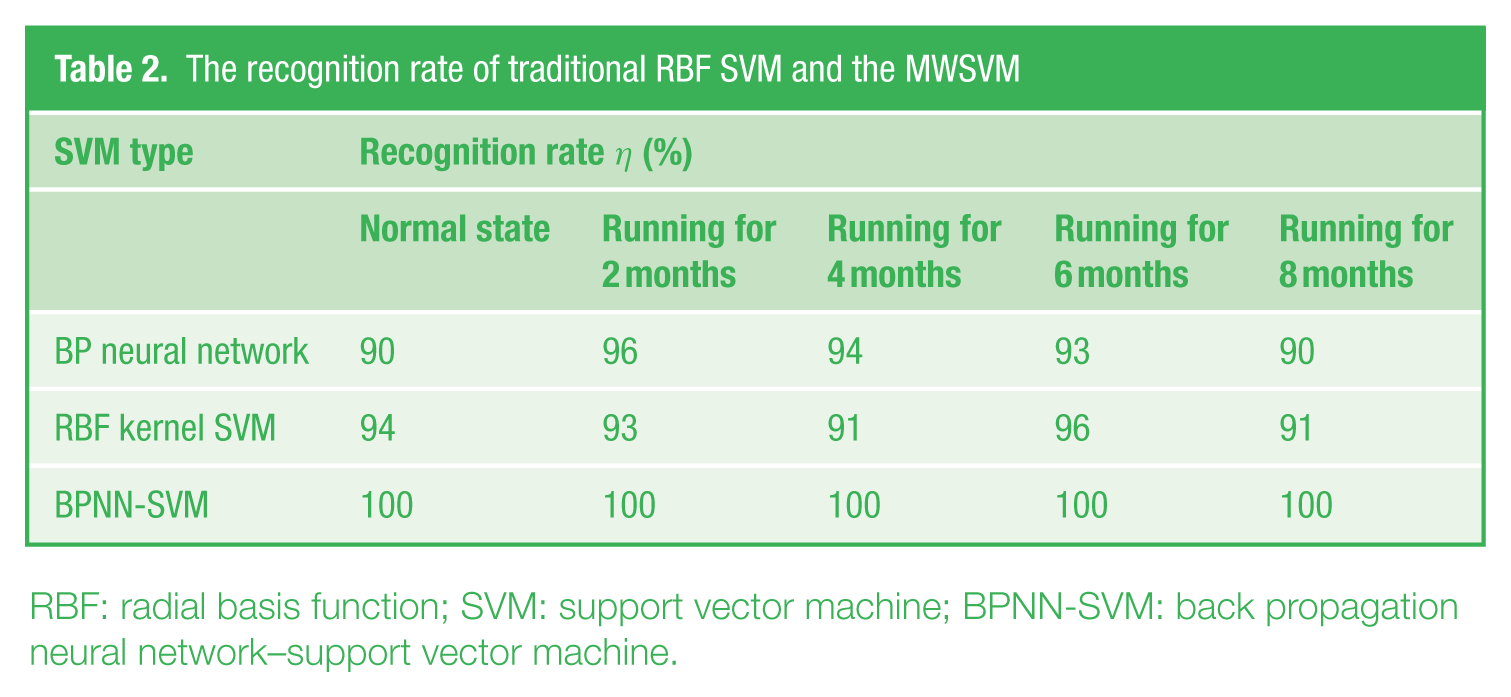
RBF: radial basis function; SVM: support vector machine; BPNN-SVM: back propagation neural network–support vector machine.

Table 2 shows that the method based on BPNN works less effective than other methods, because the method cannot extract the comprehension useful information, in addition the Neural Network also works unstable. The method of RBF kernel SVM works better than the BPNNv method, however, because the extract feature by the LPP inputted the SVM directly, so there still some loss of recognition rate. The BPNN-SVM can better identify and approach the sensitive features because of the BPNN-SVM for deal with the features effectively. Thus, the choice of BPNN-SVM to determine the bearing running states can effectively improve recognition accuracy.

V. Conclusion

First, this research used the EMD Shannon entropy method to extract the original features from the vibration signals. The LPP was used to reduce the dimension and data redundancy of the entropy features. Through those methods, the typical features could be extracted effectively.

Then, in order to more accurately identify the bearing running state, the BPNN-SVM recognition model is used so as to improve the recognition accuracy of BPNN or SVM effectively.

Third, through different comparisons we can see that the proposed method makes good use of the advantage of all parts and together to obtain better recognition accuracy and efficiency.

Finally, through the tested signals in the research, the results show the significant efficacy of the proposed method in identifying the bearing running state.

Footnotes

Acknowledgements

The authors are grateful to the anonymous reviewers for their helpful comments and constructive suggestions.

Funding

This research was supported by the National Natural Science Foundation of China (Nos 51405047, 51405048), Natural Science Foundation Project of CQ cstc2013jcyjA70012. China Postdoctoral Science Foundation funded this research, Project no. 2014M552316.

References

Dybala

Zimroz

Rolling bearing diagnosing method based on Empirical Mode Decomposition of machine vibration signal. Applied Acoustics 2014; 77: 195–203.

Zheng

Cheng

Yang

Luo

A rolling bearing fault diagnosis method based on multi-scale fuzzy entropy and variable predictive model-based class discrimination. Mechanism and Machine Theory 2014; 78: 187–200.

Mallat

A theory for multiresolution signal decomposition. The wavelet representation. IEEE Transactions on Pattern Analysis and Machine Intelligence 1989; 11: 674–93.

Yang

Cheng

A fault diagnosis approach for roller bearing based on IMF envelope spectrum and SVM. Measurement 2007; 40: 943–50.

Roweis

Saul

Nonlinear dimensionality reduction by locally linear embedding. Science 2000; 290: 2323–6.

Belkin

Niyogi

Laplacian Eigenmaps for dimensionality reduction and data representation. Neural Computation 2003; 15: 1373–96.

Tenenbaum

Silva

Langford

A global geometric framework for nonlinear dimensionality reduction. Science 2000; 290: 2319–23.

Niyogi

Locality preserving projections. In Proceedings of the conference on advances in neural information processing systems, Vancouver, BC, Canada, 8–13 December 2003, pp.1–8. Cambridge, MA: MIT Press.

Tian

Wong

Safaei

A neural network approach for remaining useful life prediction utilizing both failure and suspension histories. Mechanical Systems and Signal Processing 2010; 24: 1542–55.

10.

Roy

Mahapatra

Rani

Pandey

Dey

KN.

Robust feedforward and recurrent neural network based dynamic weighted combination models for software reliability prediction. Applied Soft Computing 2014; 22: 629–37.

11.

Vapnik

Statistical Learning Theory. New York: Wiley, 1998.

12.

Zhang

Yang

Zhao

Linear local tangent space alignment and application to face recognition. Neurocomputing 2007; 70: 1547–53.

13.

Shao

J-D

Rong

Lee

JM.

Generalized orthogonal locality preserving projections for nonlinear fault detection and diagnosis. Chemometrics and Intelligent Laboratory Systems 2009; 96: 75–83.

Rotating Machine Fault Diagnosis Based on Locality Preserving Projection and Back Propagation Neural Network–Support Vector Machine Model

Abstract

I. Introduction

II. Feature Extraction

A. EMD energy entropy calculation

B. The manifold learning method LPP

III. The BPNN-SVM Model for Fault Diagnosis

A. The BPNN-SVM model

B. The SVM parameters’ selection

IV. Validation

V. Conclusion

Footnotes

Acknowledgements

Funding

References