
Abstract
This article describes an acoustic system to visualise the location of partial discharges in electric power equipment. The system consists of an acoustic sensor array, a signal acquisition system, and signal-processing algorithms. The final result is an acoustic image of the sources of partial discharges that can be superimposed over an optical image. This study describes the characteristics of the sensor array, the processing algorithms used to locate sources of partial discharges, and the experimental performance results.
I. Introduction
With the increasing reliability required of high-voltage equipment by electric power generating companies, evaluating the reliability status of insulating elements has become a very important issue. From the point of view of diagnosing problems in electrical equipment, the location and magnitude of the partial discharges (PDs) provide an indication of the electrical insulators status associated with defects. 1
The focus of this study is to identify the location of PDs or corona-generated electrical noise present in electrical equipment using acoustic signals generated by this phenomenon.
PDs are electrical discharges that partially trace the insulation between conductors, which may or may not occur adjacent to the conductors. PDs occur at the point where the intensity of the electric field exceeds the maximum dielectric strength of the insulation. 2
The PD phenomenon materialises through changes in different types of physical variables: chemical, electrical, mechanical, electromagnetic, thermal, and so on; these changes are produced by different types of stresses. The degradation of the insulation is caused by the sum of the interactions of all of these stresses.
When PDs occur at a certain point, there is a stream of current flow that causes an instantaneous increase in temperature and a rapid increase in mechanical energy that propagates through the insulation in the form of pressure waves; this is why acoustic sensors can be used to detect this phenomenon. 1
There are several techniques that can be used to locate sources of acoustic emissions, which analyse signals detected by a sensor array to pinpoint the sources.
The triangulation technique is one of the most popular techniques used to locate acoustic sources. This technique uses three or more acoustic sensors and measures the arrival times of acoustic signals at the different sensors to calculate the coordinates of the sources, where the propagation velocity of the sound in the medium is considered. 3
This study reviews a passive monitoring technique that uses an acoustic source location technique in an isotropic medium using the relationship of magnitudes detected by an array of four sensors. Given that ‘an image is worth 1000 words’, the objective of the proposed PD visor is to build an acoustic image that represents the location of the PDs.
The study discusses the operating principle of the PD visor, which is used to build a composite image based on superimposing a synthetic sonic image of the PD sources on a photographic image of the object being analysed. In addition, the characteristics of the PD visor are described, which consist of the following: an array of four acoustical sensors, the electronics instrumentation used to amplify and filter signals, the means of digitalisation, and the algorithms used to process and synthesise the acoustical image of the PD sources.
II. PDs
PDs occur, as previously mentioned, in insulators of electrical equipment subjected to high voltage. This phenomenon takes place in dielectric ruptures, which are localised in small regions of the electrical insulator that is subjected to the high voltage. PDs cause damage by wearing out and carbonising the insulator, which eventually favours the occurrence of an electrical arc between the conductors. 2
There are three types of PDs:
Corona noise, which occurs on the surface of conductors and in the surrounding gas, where there is a large electrical field gradient. Corona noise is found on the tips or edges of conductors, produces ozone when surrounded by air, and corrodes surfaces. This type of PD takes place in conductors with gaseous insulators, such as air or sulphur hexafluoride (SF6). It is advisable to locate and eliminate sources of corona noise by adequately adjusting the electrical field distribution.
External or superficial discharges are produced on the surface of insulators and generate conduction paths or tracking, which reduces the capacity of insulators and is associated with contamination and humidity. It is important to detect external discharges promptly to avoid long-term damage.
Internal discharges are produced in the interior of insulating materials and are associated with cavities and contaminants within the insulating material. This type of discharge is only slightly related to the acoustical signal energy into the gaseous medium, and therefore, its detection requires sensors to be coupled with the solid.2,4,5
PDs produce impulsive-type sound waves, and the produced frequency band varies from the audible range up to 200 kHz.
The acoustical coupling between the different materials in electrical equipment is a relevant factor; hence, it is important to understand how acoustical waves propagate at the location of PD sources. The intensity of acoustical waves decreases as the distance from the PD sources increases. When an acoustic signal propagates from one medium to another, there is a difference in acoustic impedance that produces reflections and refractions. Only a fraction of the incident signal is propagated to the second medium. For example, the transmission coefficient between oil and steel is 0.11, and between air and steel is 0.0016. 6
III. Operating Principle and Construction Details
In contrast with methods that use the arrival times of acoustic signals to the sensors,3,7 this study uses the relationship between the magnitudes estimation and detection of the acoustic signals coming from each of the sensors in an array of three or more sensors. Figure 1 shows two acoustic sensors, S1 and S2, located on a plane and arranged at an angle ‘α’ to each other, which is referred to as the aperture angle of the device or acoustic vision angle. Acoustic sensors S1 and S2 exhibit a sensitivity pattern graphed as two circles, which are labelled H1 and H2, respectively. A source of PDs is located within the acoustic visual angle ‘α’. The source of PDs produces an acoustic component C1 over the S1 sensor and component C2 on sensor S2. Using the relationship between the magnitudes of components C1 and C2, the angle ‘θ’ can be defined, which defines the location of the source of PDs on a plane within the acoustic vision angle ‘α’. It is assumed that the acoustic signals coming from the PD sources must arrive at the sensor as a pressure plane wave.
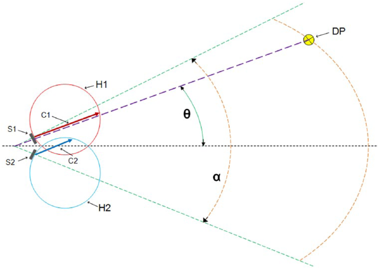
Arrangement of two acoustic sensors on a plane and a PD source
A. Sensor arrays
To locate the PD sources in a three-dimensional space, at least three sensors are required,8–10 which are arranged to form a cone with an angle ‘α’ less than 90° with respect to the directions of the maximum sensitivity of the acoustic sensors.
Figure 2 shows an array of four sensors, distributed with an angle of 30° with respect to the vertical axis and an angle of 90° to each other in the horizontal plane.
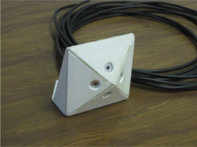
Arrangement of four acoustic sensors with an angle of 30° with respect to the axis of the arrangement
Each sensor of the array is formed by an omnidirectional microphone that includes an integrated amplifier with a sensitivity of −44 ± 2 dB to 1 kHz, a bandwidth of 100 Hz to 20 kHz, a signal-to-noise ratio (SNR) greater or equal to 60 dB, a load resistance of 2.2 kΩ, a diameter of 9.7 mm, and a height of 4.5 mm.
Once the electrical signals are acquired from the sensor array shown in Figure 2 , the signals are processed to obtain the acoustic image of the PD sources.
A photographic image is the visual two-dimensional representation of real objects in a three-dimensional space. Similarly, the acoustic signal sources and their location in three dimensions can be represented in a two-dimensional plane.
Constructing the acoustic image only requires the coordinates (x, y) to be determined on a perpendicular plane to the vision angle, as shown in Figure 3 . This figure shows a PD source that is located in a three-dimensional space and is represented, as an acoustic image point, in a two-dimensional plane.
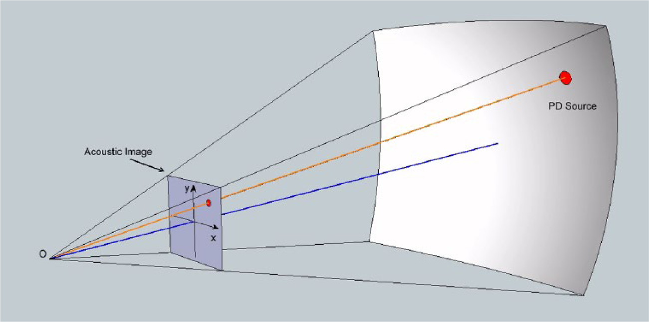
Schematic diagram of how the acoustic image is formed
Just as photographic images have aperture angles, the angle formed by the acoustic sensors determines the aperture angle of the acoustic image. By matching the aperture angle of an optical camera with the aperture angle of a sensor array, it is possible to superimpose both images, as shown in Figure 4 .
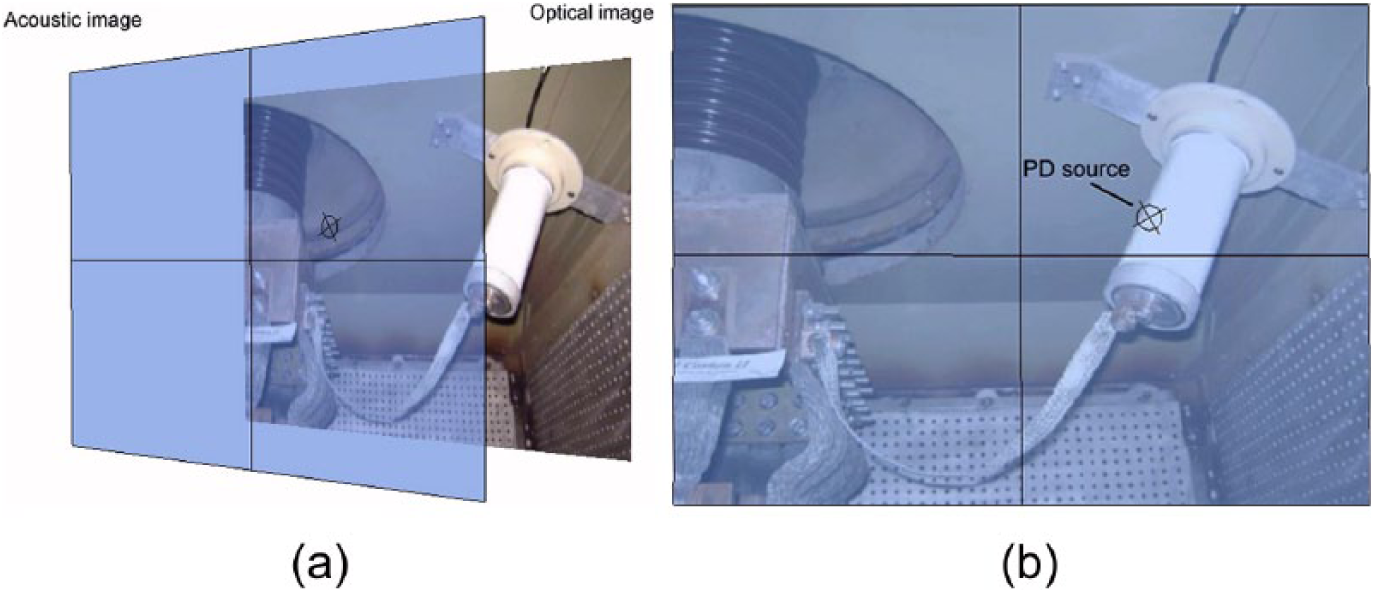
The acoustic and optical images, shown (a) separately and (b) superimposed
The vision angle of the sensor array corresponds with the angle of the video camera oriented vertically and horizontally, such that it is possible to superimpose the synthesised acoustic image and the real signal obtained from the video camera.
Distortions and deformations of the optical images are also present in acoustic images; these problems can be corrected using calibration patterns and image processing.
IV. Data Acquisition and Signal Processing
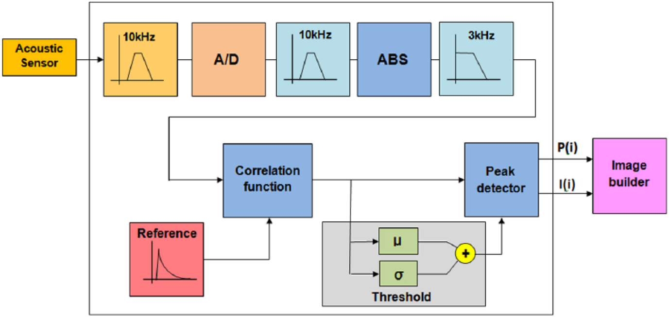
The data acquisition and signal processing of acoustic signals are performed independently for each sensor in the sensor array as it is shown in the block diagram of Figure 5 .
Block diagram of the processing of acoustic signals from each sensor in the arrangement
A. Analogue signal processing
The signals provided by the sensor array require amplification and must be limited to their band of frequencies to enhance the SNR. The principal reasons are noise reduction, since PDs are characterised by the generation of impulsive sonic noise with spectral components in a wide spectrum of frequencies; the directionality of acoustic sensors, which improves as the frequency of the sonic signals increases; and aliasing, to avoid the ‘aliasing’ effect when performing digitalisation. Therefore, analogue signals are carried out using individual band-pass filters with a central frequency at 10 kHz where Q = 10.
Filtered signals can be digitalised with a sampling frequency of 50 k samples per second with a resolution of 16 bits using a commercial data acquisition module (DAM). A total of 834 samples are acquired by each channel, which corresponds to a cycle of 60 Hz or 16.66 ms, that form four vectors, X1(n), X2(n), X3(n), and X4(n).
The DAM transfers the information to a computer through a USB port, and the acquisition may or may not be synchronised with a reference phase signal with which the electrical equipment being analysed is excited. A video camera located in the sensor module in the central part of the acoustic sensor array is interconnected directly with the computer through another USB port.
B. Signal processing
Once the analogue to digital conversion is performed, signal-processing algorithms are implemented in a computer using a proprietary software application developed via a graphical language.
Figure 5 shows schematically the processing block sequence; however, these blocks can be described as follows: a second-order Butterworth-type band-pass filter, with central frequency at 10 kHz, was implemented and the absolute value (ABS) is obtained; a low-pass filter with cut-off frequency at 3 kHz is carried out, which provides the envelope of the acoustic entry signals in the form of a vector X(n) with ‘n’ samples; a constant reference signal is created in the form of vector K(m), which is obtained from the particular response of the previous processing produced by a typical PD; the cross-correlation function C(n) is performed by computing the following operation:
The cross-correlation function results are transferred to a peak detector and to an adaptive threshold detector. The adaptive threshold detector calculates the threshold of detection using statistical parameters, such as the mean and standard deviation of the signals at the output of the correlator, and establishes the detection threshold used to discriminate in the peak detector; consequently, the peaks detected below this threshold are ignored. The peak detector yields two vectors: the magnitude of the peak values ‘p(i)’ and the index vector ‘i’, where the maxima values within vector ‘p(i)’ are found.
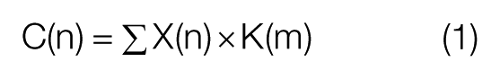
Figure 6 shows the module that creates the acoustic image. The module receives the information from each of the signal-processing modules, the magnitudes, and the P(i) and I(i) indices, respectively, which represent the time of arrival of the PDs to each acoustic sensor.
Schematic diagram of the acoustic image builder module
The set of maximum values associated with each sensor is sent to the module that calculates the coordinates associated with the acoustic image within the calculation module of the acoustic image. Additionally, the set of indices from the signal-processing modules is processed in the index validation module. This module verifies that the indices exhibit a standard deviation of less than 2.0, which indicates that the maxima values are related and the calculated coordinates in the coordinate calculation module are valid. This validation eliminates false detections produced by undesirable reflections or spurious noise.
The coordinate calculation module obtains the coordinates where the PD sources are located using the relationship between the magnitudes of the peak values. In contrast to the techniques that use triangulation by solving non-linear quadratic equations, which requires considerable processing time, the proposed technique only uses the relationship between the maximum measured values. The module that constructs the acoustic image uses the coordinates calculated in the coordinate calculation module and builds the acoustic image only if the indices of the maxima are validated by the index validation module.
The acoustic image is formed by a two-dimensional plane, in which the locations of the set of detected PDs are graphed. The acoustic image is finally shown on a computer screen or information processing equipment.
Given that this method allows for a processing velocity that is two orders of magnitude greater than that in triangulation techniques, the acoustic image can be refreshed many times each second, which gives the impression of being graphed in real time.
V. Experiments and Results
An experimental setup for testing the PD image visor was carried out in the laboratory using a PD simulator, four acoustic sensors, a DAM, and a personal computer. The DAM is connected via USB to the personal computer for performing signal-processing algorithms. Figure 7 depicts the experiment setup.
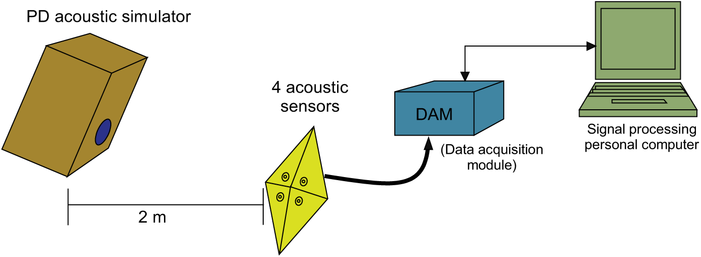
Experiment setup for testing the partial discharges image visor
A PD simulator was developed, which generates impulsive acoustic noise with a repeat frequency of 120 Hz. The PD simulator is placed at a distance of 2 m from the sensor array. Figure 8 shows a photograph of the PD simulator mounted on a commercial tripod. The simulator is powered by a 9-V battery and allows calibrating the calculation algorithms without requiring any actual energised equipment. The simulator consists of a simple oscillator that generates a square signal with a working cycle of 50%, where the output signal is derived and fed to a piezoelectric transducer.
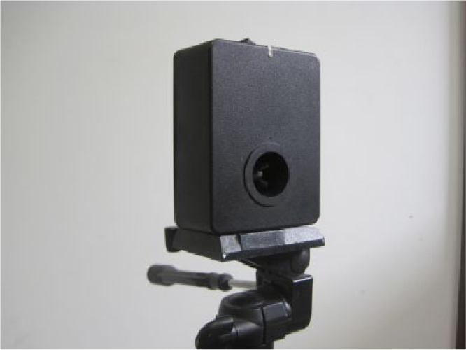
Acoustic PD simulator mounted on a commercial tripod
A series of experiments were conducted in the laboratory using the experiment setup to assess the different blocks that comprise the PD image visor. Figure 9 shows a typical PD acoustic response measured after being digitalised, when entering to signal-processing module. These signals are the result of the analogue band-pass filtering with central frequency at 10 kHz, once they have been amplified and digitalised.
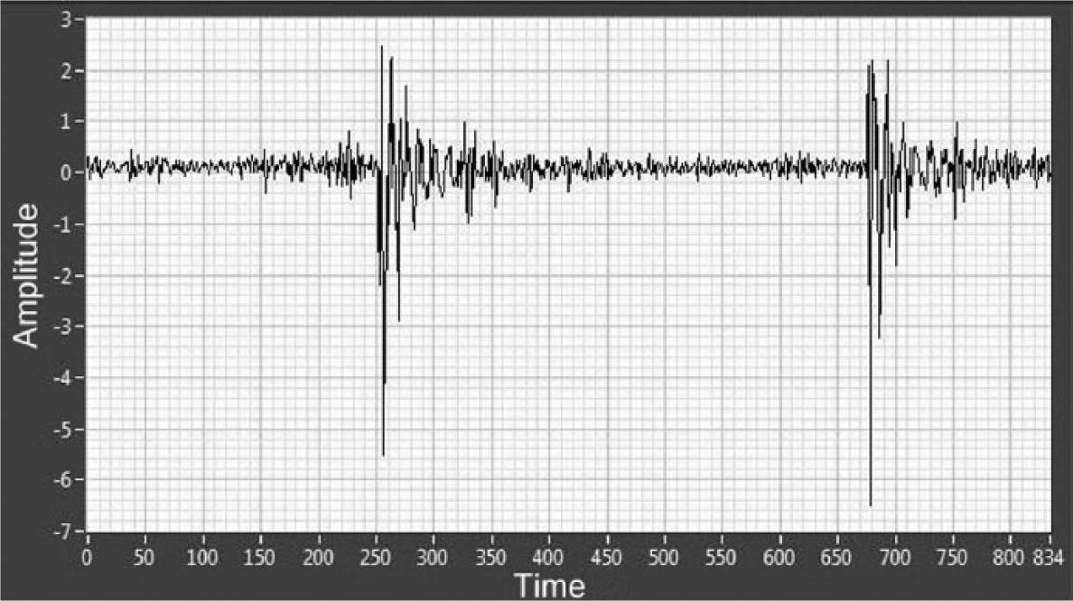
Typical PD acoustic response measured after being digitalised
The reference signal used to obtain the cross-correlation function, which is made of 30 elements in length, is shown in Figure 10 . This wave shape corresponds to the absolute value of the envelope of the impulse response of the sensor array, amplifiers, and filter applied to the entry signal. Its magnitude is normalised such that the sum of its elements is equal to unity.
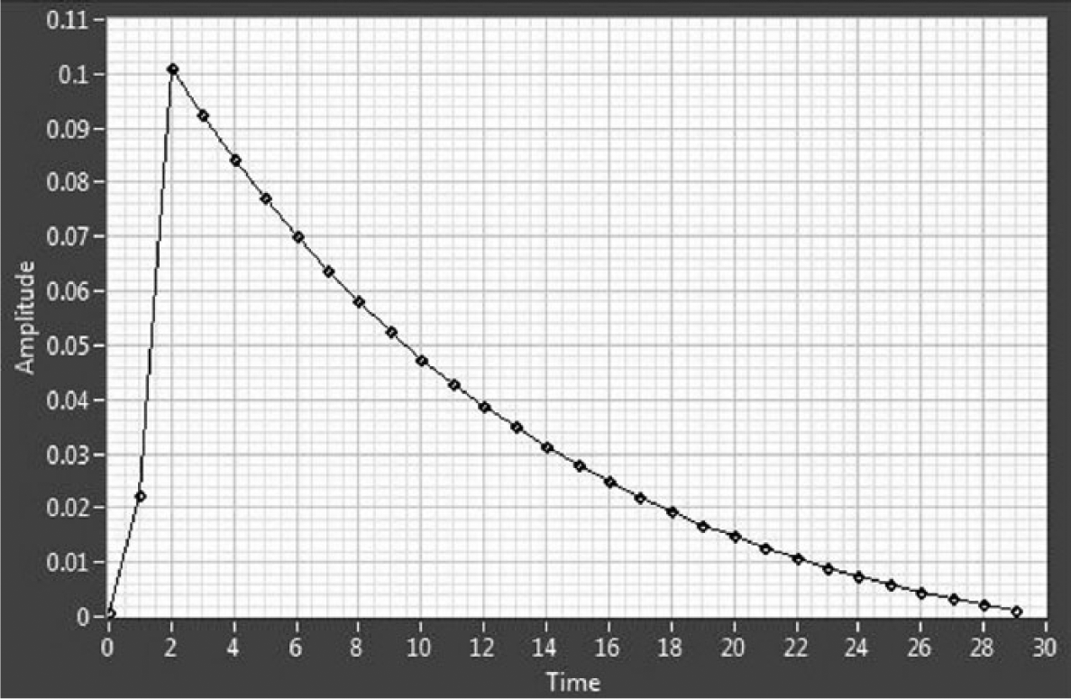
Reference signal used by the correlator
The output signals of the correlating module and the threshold value yielded by the adaptive threshold detector are shown in Figure 11 . The threshold is calculated for all signals, and at every time instance, the acoustic signals are acquired. Figure 11 exhibits the SNR enhancement, associated with the signal-processing algorithm, compared to the PD acoustic signals shown in Figure 9 .
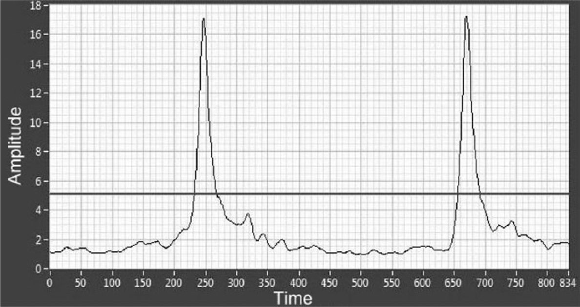
The same acoustic signal in Figure 7 taken at the output of the correlator with the detection threshold
Calibration of the PD visor is performed using the aforementioned simulator. This source is placed at a distance of 2 m away at three positions: at an angle of 0° horizontal and vertical; 30° horizontal, 0° vertical; and 30° with 0° horizontal vertical and with respect to the direction of the sensor module. The control program selects the calibration mode, and three measurements are performed. These measurements are used to adjust the gains of the four channels and also to establish the detection limits of the PD sources.
A laboratory setup arrangement of PDs coming from a power generator bar was carried out. Figure 12 shows this arrangement.
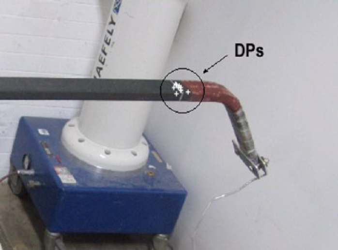
Laboratory detection of PDs coming from a power generator bar
Figure 12 depicts a screen of the PD image visor, where the PDs are shown by white marks over the power generator bar under test.
VI. Conclusion
A PD image visor using an acoustic sensor array has been designed, implemented, and evaluated. The PD image visor comprises four acoustic sensors, a DAM, and a personal computer that executes signal-processing algorithms. The effectiveness of the proposed technique was tested in the laboratory using a PD simulator and a power generator bar. To corroborate the results produced by the PD image visor, the acoustic images were superimposed over an optical image. The employed signal-processing techniques, based on the cross-correlation function, improve the SNR by reducing interference and background noise. Due to the impulsive and repetitive properties of the acoustic signals generated by PD sources, the image visor described in this work has shown to be adequate for detecting their location. Future work considers implementing several criteria for handling multiple sources in space and time and the application of this technique with a sensor array immersed in oil inside a power transformer.
Footnotes
Funding
This research received no specific grant from any funding agency in the public, commercial, or not-for-profit sectors.