
Abstract

I. Introduction
Stable control is essential for the safe and efficient operation of industrial processes. Understanding the basics of process control is essential for the instrument engineer or technician to effectively design, maintain and tune instrumented control loops with confidence.
All processes contain, in various proportions, the dynamic elements dead time and capacity. Dead time is the interval, after the application of an action, during which no response is observed and capacity is a location where mass or energy can be stored. These dynamic elements determine the way control loops behave in terms of speed of response and stability.
Each process parameter exhibits unique properties that determine the ease of control and the control strategy to be applied. Flow and liquid pressure loops exhibit low capacity and no dead time, giving fast and noisy characteristics requiring a low gain (wide proportional band) response with reset (integral action) to maintain a desired value.
Gas pressure loops usually exhibit high capacity and no dead time, with slow characteristics, requiring a high gain (narrow proportional band) response to maintain a desired value. Liquid-level loops exhibit high or low capacity and variable dead time, giving fast or slow, noisy (boiling) and lag characteristics requiring medium gain and in certain applications (boiler level control) reset response to maintain a desired value. Temperature loops can exhibit high or low capacity and dead time, giving fast or slow and lag characteristics requiring variable gain, reset and anticipatory (derivative) response to maintain a desired value.
The process plant design and the control philosophy should be considered throughout a project design process. For example, if a processing unit takes a long time to achieve stable and optimal operating conditions, the feeds should be held constant by the use of surge tanks in which the level is allowed to float between acceptable limits.
II. Control Loop Presentation
A loop schematic or process control diagram is a single line diagram used to identify the basic specifications and structure of an instrument control loop and is developed from the Process & Instrumentation Diagrams (P&ID). A completed loop schematic diagram should provide all the details necessary to enable the loop interconnection drawings to be prepared correctly.
The main features include unique identification and specification of all components in the loop, the location of the components, signal interconnection type, power and air supply type and source. Cable, wiring and termination details are excluded. Symbols are defined using international standards according to Instrument Society of America (ISA) or British Standards (BS):
BS 1646-3:1984 Symbolic representation for process measurement control functions and instrumentation.
American National Standards Institute (ANSI)/ISA-5.1-2009 Instrumentation Symbols for Identification
Each element within the loop is identified by a symbol containing the unique identification (Tag Number). The symbol used defines the function, accessibility and the location as shown in the Table 1 .
Instrument schematic symbols to ISA-5.1

ISA: Instrument Society of America.
Normally accessible to the operator.
Normally inaccessible or behind panel devices.
Typical tag numbers are developed as follows:
FIC 101 Instrument identification or Tag Number;
F 101 Loop identification; function descriptor (F-Flow, T-Temperature, P-Pressure, L-Level)
101 Loop number;
FIC Functional identifier (I-Indication, C-Control, T-Transmitter, X-Miscellaneous);
The instrument loop number should convey as much information as possible, such as plant area designation and assigned blocks of numbers for specific functions. When scheduled, fields are provided to the right of the symbol to describe the component function, device manufacturer/type specification number and calibrated range. Signal levels and power or pneumatic supplies are also shown. On the P&ID, the component symbols are interconnected to show the relationship and functionality of the components with respect to each other. The line weight and format represents different signal types.
III. Control Loops
An open loop ( Figure 1 ) involves an operator manually setting a signal to manipulate a control device, such as a control valve or a variable speed drive to manipulate a process variable. The result of this action may be monitored by a separate measurement and indication loop.

Open loop control
A closed loop ( Figure 2 ) incorporates feedback of the process measurement to a controller, which is assumed to be a proportional, integral and derivative (PID) controller, with the desired value of the process variable being the set point of the controller. The basic control loop consists of an instrument measuring a process variable and converting it typically into a 4–20 mA direct current (DC) signal for transmitting to a controller. The controller produces a 4–20 mA DC output signal, the value of which is dependent, on the error between measurement and set point and the settings PID. The output signal is connected to an actuator, such as a control valve or variable speed drive.

Closed loop control
IV. Fail-Safe Control
Controller output direction in response to an error (±) is determined by the controller action.
Direct action control (input direction referring to set point). Increasing input gives an increasing output – decreasing input gives a decreasing output.
Reverse action control (input direction referring to set point). Increasing input gives a decreasing output – decreasing input gives an increasing output.
Control valve failure action is determined by the process, for example, a heating valve is usually fail closed and a cooling valve is usually fail open. A ‘fail closed’ valve requires an increasing controller 4- to 20-mA output to open the valve, and a fail open valve requires an increasing controller output to close the valve.
An incorrect match of controller action and valve action will give positive feedback, with the controller output driving to a maximum or minimum signal output, which in turn could lead to a potentially dangerous process condition.
Correct control valve actuator specification is critical to obtaining correct ‘fail safe’ operation. Pneumatic actuators should be specified ‘Air fail open’ or ‘Air fail closed’ to cater for both failure of the positioning signal or the valve air supply. Electric and hydraulic control valve actuators require either a spring or backup source of power to ensure fail safe action.
V. Three-Term (PID) Controller
Typically, process controllers can have the following configurations:
On–off – A narrow proportional band effectively provides on–off control;
Single term – proportional band (P);
Two term – proportional + integral action (PI);
Three term – proportional + integral action + differential action (PID).
A simplified algorithm for a three-term controller with control modes Proportional, Integral and Derivative, which does not exhibit interaction between control modes, is shown

where P is the proportional band, %; Ti is the integral action time, min (control theory basic unit is seconds); Td is the derivative action time, min; Po is the steady-state controller output; and e is the error between process measurement and set point. (Note: In control theory, the basic unit for the time constant is seconds.)
Inspection of the controller equation leads to the following conclusions regarding the controller output, which should be remembered when tuning controllers:
If there is no error, the controller output equals the steady-state output Po.
The controller gain is 100/P. Increasing P decreases the controller gain.
Considering the integral term being 1/Ti, increasing Ti reduces its effect.
Decreasing the derivative term Td setting reduces its effect.
In practice, manufacturers’ controller algorithms can exhibit unique behaviour as follows:
The controller output will exhibit derivative kick when the Td term operates on the error due to set point change.
The derivative term may be taken from the controller output.
Integral wind up protection against sustained error on a controller with integral action.
VI. Control Loop Tuning
When tuning control loops, it is important to understand the impact the tuning parameters will have on the process. The following ground rules are given for guidance.
Safe setting values are as follows:
Proportional band P, %, highest value (minimum gain);
Integral action time Ti, min(s), longest time (or off);
Derivative action time Td, min(s), shortest time (or off).
A wide proportional band should be used on noisy signal control loops, for example, liquid flow, liquid pressure and level; note the controller gain is 100/P. Integral action times (Ti) are used to eliminate error; short times can make the loop less stable. Derivative is never used on noisy signals as Td operates on rate of change of error de/dt, where rapid changes in error will result in large rapid changes in controller output leading to control valve slamming and damage.
A. Proportional band (P)
The proportional band setting determines the magnitude of the controller output change as a result of the error between the process measurement and the controller set point. There is no error at one specific process load condition:
Use a narrow P in the range 1%–50% on slow processes: Gas pressure, temperature and vapour pressure control
B. Integral action time (Ti)
Integral Action Time changes the controller output signal at a rate proportional to the magnitude of the error until the error is eliminated. It should never be set so fast that the resulting load change exceeds the process response characteristics which will result in the controller driving to its maximum or minimum output:
Use a low Ti in the range 0.05–2 min on fast and noisy processes: flow and liquid pressure.
Use a high Ti in the range 2–120 min on slow processes: temperature, vapour pressure and composition control.
It is used on critical level control applications such as boiler drum level and distillation column reboiler level control, where settings are application specific. It is not used on liquid level control where a specific control point is not required, thus allowing for steady flow conditions, for example, surge tanks between process units. The use of Ti is often unnecessary on gas pressure control.
C. Derivative action time (Td)
Derivative Action Time changes the controller output at a rate proportional to the rate of change of the error de/dt and provides an anticipatory characteristic.
The controller action can be likened to that of an experienced operator adjusting a heating valve to achieve a set value as fast as possible. Not normally used on noisy processes such as Flow, Liquid Pressure and Liquid Level.
The fast rates of measurement change can lead to control valve slamming and damage. Td is typically used on Temperature, Vapour Pressure and Composition and should be set conservatively (short Td) to protect against control instability resulting from unanticipated load changes. Td usually set in the range Ti/6 < Td < Ti/2 is considered reasonable.
D. Integral action time saturation (wind up)
When a sustained error is maintained between the set point and the measured variable on a controller with Ti, the output will drive off scale (valve full open or closed). This condition is typical of heating and cooling a batch reactor to a desired temperature and composition endpoint control. Controllers incorporating Proportional and Derivative modes only do not experience this problem. Modern controller designs employ nonlinear techniques to prevent the integrator output becoming too high.
E. Controller tuning methods
There are many practical and theoretical approaches to controller tuning. Modern controllers are provided with auto-tune facilities which should be applied with caution on new systems. A long established procedure due to Ziegler and Nichols known as the Ultimate Sensitivity Tuning Method will produce conservative parameters allowing for further final fine tuning.
Set the control modes to their minimum effective values: that is, maximum P, maximum Ti and minimum Td (or off). Reduce P while making small set point changes in both directions until the measured variable begins to oscillate at constant amplitude, providing a trend reading of the proportional band Pu and the oscillation period Tu. Initial controller settings are determined from Table 2 .
Initial controller settings

This procedure can be used as a ‘starting point’ for tuning control systems on batch or continuous processes, Tu being established at a stable condition. The following plot ( Figure 3(a) ) shows the process simulation to study the effect of tuning parameter settings ( Figure 3(b) ) when controlling level in a surge tank with a controller set point of 2 m. The initial inlet flow is set at 4000 kg/h with a step change to 16,000 kg/h after 15 min and then back to 4000 kg/h after 50 min.

F. Interpretation of Figure 3 trends (note that derivative mode is not used due to the noisy signal)
P only set at 25%. Initial error is 0.1 m. There is a specific flow condition that will result in zero error. The level increases to 2.47 m and then returns to 2.1 m.
P only set at 10%. Initial error is now reduced to 0.04 m. The level increases to 2.2 m and then returns to 2.04 m. Reduced P has reduced the error as a result of the load change.
P set at 25% and Ti set at 5 min. This eliminates the error. The initial deviation is 2.24 m, with the error being eliminated after 30 min.
P set at 25% and Ti set at 2 min. This reduces the time to eliminate the error, but the controller is now more responsive and is approaching its limits. A further reduction in Ti would result in the tank level cycling.
VII. Advanced Control Loop Configurations
Single-loop control systems have limited application, with more advanced control systems requiring multiple loop configurations. The more common of these multiple loop systems are shown in Figure 4 .

Multiple loop control
A. Cascade control
The output of one controller, the primary or master, manipulates the set point of another controller, the secondary or slave. Each controller has a separate measurement, and the secondary controller manipulates the controlled device.
The principle advantages are that process upsets in the secondary loop are corrected before they can influence the primary measurement and lags existing in the secondary loop are reduced, improving the speed of response. Also, the secondary loop provides exact manipulation of the mass or energy balance by the primary controller. The secondary loop process variable must respond faster than the primary loop process variable. The simplest example of a cascade loop is a control valve fitted with a positioner.
A temperature loop is frequently cascaded to a flow loop. When a differential pressure type of measurement is used, for example, an orifice plate, the flow measurement signal is normally linearised by square root extraction, in order to provide acceptable control.
An example of the application of cascade control is shown in Figure 5 , depicting steam boiler drum-3 element level control, in which the boiler feedwater flow set point is set equal to a steam flow and the level controller trims the boiler feedwater flow controller in cascade to maintain a material balance.

Steam boiler drum-3 element level control
B. Ratio control
Ratio control is frequently used in ingredient control where any number of streams can be set in ratio to one independent stream which is set according to production requirements. This type of system is used in gasoline blending, bio-fuel additive control, furnace air-to-fuel ratio control and composition control in many industries. An example of the application of ratio control is shown in Figure 6 which shows two additives being mixed with a single independent stream.
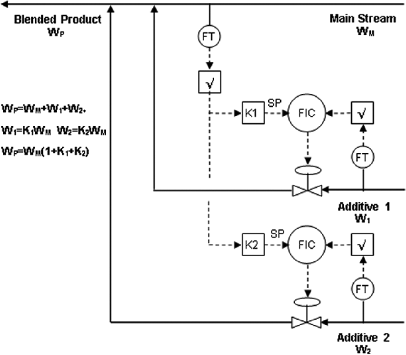
Stream blending by set point radio control
C. Auto-select (override) control
This configuration is used in the situations where two or more variables must not pass specified limits due to economy, efficiency or safety. Pipe line transfer systems require the maximum flow to be delivered subject to satisfactory operating conditions being maintained at the prime mover, be it a pump or compressor. If a selected parameter, such as suction pressure, goes below a set limit, the suction pressure controller output overrides the flow controller output via a signal selector and will control the flow.
If a processing unit is to be operated at a maximum allowable measurement parameter across the unit, where several measuring points are provided, a high selector is used to select the highest measurement for input to the controller. An example of this would be to control at the highest temperature in a fixed bed reactor or furnace.
An example of the application of auto-select control is shown in Figure 7 , which shows a system, where it is required to provide a preset steady flow to a downstream processing unit, provided there is an adequate level in the upstream surge tank. If the level cannot be maintained, the flow to the downstream unit will be cut back to maintain the surge tank level.

Auto-select (override) control
This multi-loop configuration is used in situations where two or more process variables must not cross specified limits for reasons of economy, product specification or safety
Footnotes
Funding
This research received no specific grant from any funding agency in the public, commercial or not-for-profit sectors.