Weighing without Touching: Applying Electrical Capacitance Tomography to Mass Flowrate Measurement in Multiphase Flows

Abstract

Electrical capacitance tomography has a well-established reputation as a research tool and has been used in a number of industrial applications including dry solids flows, gas–liquid flows, and wet gas flows. Electrical capacitance tomography can give detailed flow structure information that has been experimentally validated against other techniques. Here, we focus on its use for measuring the detailed flow structure and overall mass flowrate of dispersed dry solids in gravity-drop flows. Electrical capacitance tomography–based flowmeters capable of being mass-produced and deployed into the commercial industrial environment are being developed, and prototypes are available, but none are yet in full-scale manufacture. Sensors of this type are being designed for applications in milling, power generation, and pneumatic transport. The same sensor technology may also be applied to measurements of gas–liquid flows in oilfield applications.

I. Introduction

Many industrial processes involve the transport of mixtures of materials along conduits or pipes. This paper addresses the measurement of such flows, specifically the measurement of dispersed solids being moved under gravity or by pneumatic means. Gravity-driven flows are typical of milling, feedstock delivery, and hopper discharge in food, agriculture, mining, and power generation, while pneumatic transport is used in those and many other industries. The two applications share the basic problem description in that the flow contains solid particles dispersed in air, and that the mass flow of the solids is of prime interest while the air flow is incidental.

Electrical capacitance tomography (frequently abbreviated to ECT) has been used as a research tool since the mid-1990s. Early applications of ECT were to multiphase flows, but output was typically limited to qualitative pictures, and the move to quantitative measurement of flows was seen in the early 2000s. This paper addresses the application of ECT as a flowmeter for dispersed solids and describes some of the relevant background, application-specific requirements, and test results.

II. A Brief History of ECT

ECT was developed at University of Manchester Institute of Science and Technology (UMIST) in the late 1980s, largely under the impetus of Professor Maurice Beck. An early book looked to a promising future of commercial exploitation. ¹ Production of images and simulated ‘videos’ of flow conditions were demonstrated very early in the life of ECT, but industrialising its use as a flowmeter requires a level of accuracy and rigour in the measurement physics that has proved difficult to achieve. Of particular concern in achieving accurate flowrate measurements are the effect of particle shape, the moisture content of the material, and the temperature stability of the sensor. The most developed arena of measurement at the moment is in gravity-driven flows of dry solids. Here, ECT can compete with the accuracy of weighing systems by offering the advantages of non-intrusive continuous measurement.

The accuracy of ECT has been investigated by comparisons between ECT measurements and other sensors in two-phase flows. Such comparisons include ECT and gamma-ray densitometers, ² wire-mesh sensor and ECT, ³ and ECT and weight scales. ⁴ These comparisons have shown that for measuring dynamic properties of local flow, ECT is fast (up to 5000 frames of data per second), accurate, non-intrusive, but with low spatial resolution.

ECT flow sensors are made by mounting a series of electrodes around the outside of the flow of interest. The value of capacitance between many pairs of electrodes is then measured and the resulting matrix of measurements interpreted through use of a sensitivity map to give an image or tomograph, typically representing a two-dimensional slice of the pipe. The arrangement of electrodes and their size may vary, as shown in Plaskowski et al., ¹ Hunt et al.^2,3,4 and Azzopardi et al., ⁵ but here, we primarily refer to ECT sensors made up of a set of curved rectangles around the flow, either mounted inside a non-conducting liner, or outside a non-conducting liner. The application will strongly influence the details of the design. An earthed outer electrical shield is often also the main structure offering mechanical strength and pressure containment, but these functions may require separate elements.

Figure 1 shows a typical ECT research system where the sensor is mounted on a flanged section of pipe, the capacitance measurement is made in a conventional rack-type unit, and the image processing is undertaken on a laptop PC. The sensor is connected to the measurement unit by coaxial leads – the advantages of this arrangement is that different sensor heads may be used with the same electronics, and software improvements are easily incorporated. Communication between the PC and the capacitance measurement unit is via high-speed Ethernet, and thus communications are possible with a control system, but the system is typically used as a stand-alone research device.

Figure 1.

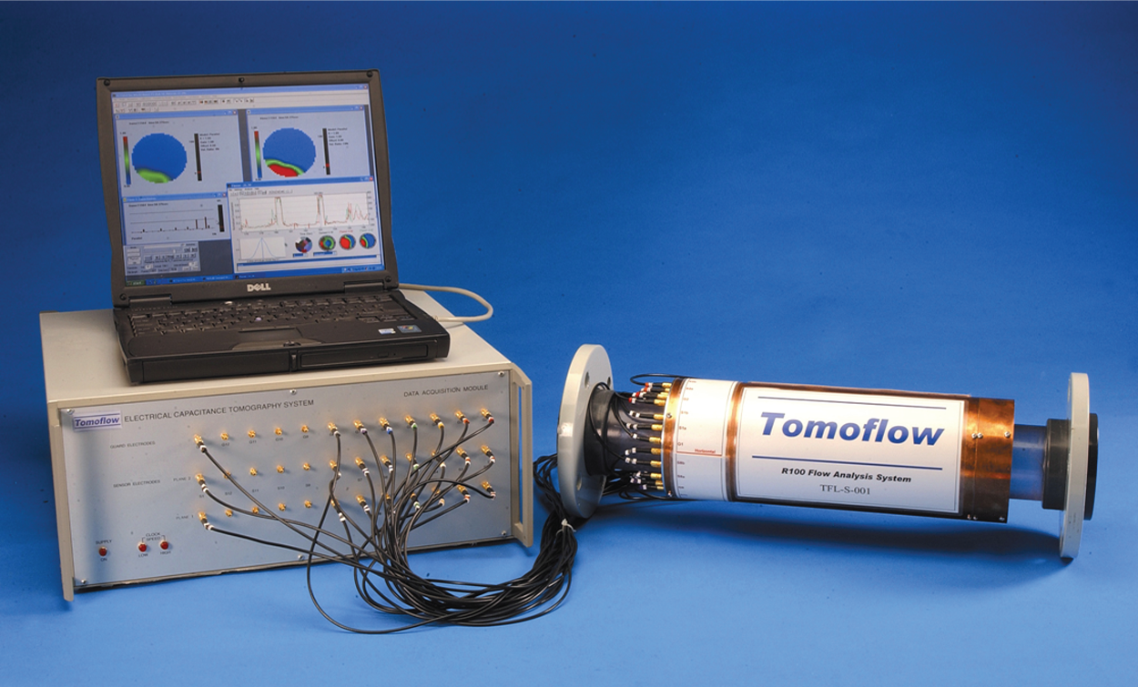
A typical ECT research system

ECT research systems have been used in a wide range of applications, including the measurement of coal feedstock, ⁵ oilfield multiphase flows, ⁶ fluidised beds, ⁷ and dense-phase conveying of polypropylene pellets. ⁸ Figure 2 shows a sensor head designed for use at 11 bar and 195 °C. Although research systems with coaxial connection may be inconvenient in many commercial contexts, there are advantages including the use of different sensor heads with the same electronics, and in the case of high-temperature measurements, the electronics may be mounted away from the hot measurement zone.

Figure 2.

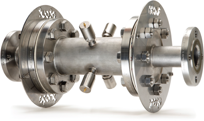
An ECT sensor designed for use at 11 bar and 195°C

An ECT flowmeter capable of being deployed into the commercial industrial environment must achieve a certain level of performance and robustness to product and process variation. It must also be packaged in such a way as to withstand the environment and communicate with the process control system. Such meters are being developed, and prototypes are available, but none are yet in full-scale manufacture. The prime difference between an ECT research system and a commercial sensor is that the commercial sensor has the electronics fully integrated into the body of the sensor, and it is designed to measure process parameters such as flowrate or density, which are then passed to a control or data logging system via the high-speed Ethernet connection. Although the commercial sensor is focussed on the measurement of specific process parameters, all the functionality of the research system is also available within it. Sensors of this type are being designed for applications in milling, power generation, and pneumatic transport.

III. ECT for Imaging and Flow Measurement

ECT systems can be used to obtain images of the distribution of permittivity inside a pipe or vessel for any arbitrary mixture of different dielectric materials. From the permittivity distribution, the distribution of the relative concentration (volume ratio) of the two components over the cross-section of the vessel is calculated. ECT is limited to applications where the continuous phase in the pipe is not highly conducting.

A typical ECT permittivity image uses a square grid of 32 × 32 pixels to display the distribution of the normalised composite permittivity of each pixel. For a circular sensor, 812 pixels are used to approximate the cross-section of the sensor. The values of each pixel represent the normalised value of the effective permittivity of that pixel. In the case of a mixture of two dielectric materials, these permittivity values are related to the fraction of the higher permittivity material present at that pixel location.

The overall volume ratio of the materials inside the sensor at any moment in time is defined to be the percentage of the volume of the sensor occupied by the higher permittivity material and can be calculated by integrating the pixel values from the image. The volume of the sensor is the product of the cross-sectional area of the sensor and the length of the sensor measurement electrodes. Images of flows are normally shown using a colour scale from blue (pixel full of low-permittivity material) to red (pixel full of high-permittivity material).

In the example shown in Figure 3 , each image represents the ‘cross-section’ of the flow (in this case, a hollow plastic sphere filled with polypropylene beads), where each ‘cross-section’ is in fact a cylinder of 3 cm long. As the sphere passes through the sensor, the image represents the average concentration of solids along the electrode length at each point in time.

Figure 3.

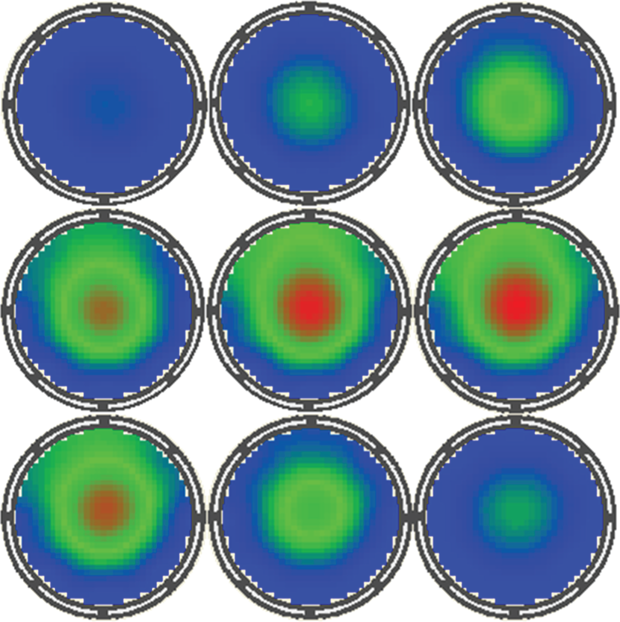
Example images from ECT on a 32 × 32 grid of false-colour pixels representing electrical permittivity. Blue is air, red is packed plastic beads, and green representing values in between. The images from top left to bottom right show the passage of a plastic sphere packed with plastic beads at intervals of 5 ms

In the following analysis, we refer to the relative permittivity (or dielectric constant) of materials. The relative permittivity of a material is its absolute permittivity divided by the permittivity of free space (or air). Hence, the relative permittivity of air is 1, and typical values for other materials in solid or liquid format are polystyrene, 2.5; glass, 6.0; wheat, 4.5–5.5; and mineral oil, 2.1–2.5.

IV. Deriving Flowrate Information

Twin-plane sensors are used in conjunction with guard electrodes to create two image ‘planes’ axially separated along the flow (see Hunt et al. ⁴ for more details). As described above, each ‘plane’ is in fact a cylinder of finite length made up of 812 pixels on a 32 × 32 square mesh so that each pixel represents the spatial average of concentration in a square cylinder a few centimetres long. In the case of typical flow-line sizes (5-cm to 20-cm diameter), the pixel cylinder is of high aspect ratio – between 5 and 20 times longer than wide.

Given the relatively low spatial variation of velocity fields in pipe flows, and the computation required to derive velocity information from each of the 812 pixels, it is more realistic to divide each image plane into a number of zones arranged appropriately for the flow conditions. For 8-electrode systems, dividing the flow into 13 zones as shown in Figure 4 gives zones containing approximately 62 pixels each and which have typical length scales of D/4 both within the cross-section and axially along the pipe, where D is the pipe diameter. These zones are more consistent with the linear spatial resolution of ECT, which is sometimes quoted as D/n_e, where n_e is the number of electrodes circumferentially around the pipe, in this case 8. Within each zone, the pixel values are averaged to give one concentration value per zone for each frame of data. Flows can then be measured with the sensor, and the concentration per zone may be calculated.

Figure 4.

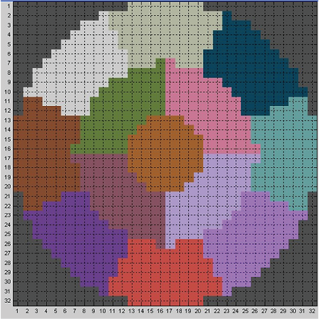
Typical zone map for flow measurement purposes

An example of the resulting time-concentration plots is shown in Figure 5 . The concentration from each plane is shown at each point in time, in this example from the gravity-drop flow of wheat in a small test facility. There are n possible plots of this type for each data set, where n is the number of zones used – in this case 13. Note that while there is some noise on the signal seen in the no-flow zones at the beginning and end of the data set, the major variation shown in the red and green lines on Figure 5 is primarily real flow information, as demonstrated by the following analysis.

Figure 5.

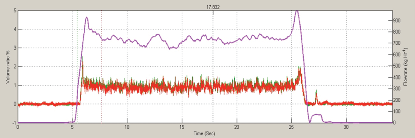
Average concentration (red line and green line – left axis 0%–5%) and 1-s averaged flowrate (pink line – right axis 0–1000 kg/h) for wheat at 11% moisture, 750 kg/h average flowrate

Simple image reconstruction techniques assume that the electric field is unchanged by the presence of varying dielectric materials inside the sensor. This means that to interpret the concentration of material from the permittivity map, the use of a capacitance model is required. Yang and Byars ⁹ present two models based on simplified cases.

The simplest case assumes that the effective permittivity of the mixture can be obtained simply by summing the effects of the two components. This is known as the parallel capacitance model and corresponds to the case where there are effectively continuous bands of each dielectric material between the electrodes of the sensor. The parallel capacitance model tends to be valid for densely packed materials, such as liquids, or powdered/granular materials in dense-phase processes.

An alternative model is required for the situation where the higher permittivity material is present in dilute quantities in the mixture. This situation occurs, for example, in lean-phase fluidised beds or pneumatic conveying applications. The model which fits this situation is the series capacitance model, where it is assumed that the effective permittivity of a mixture of two materials can be found by assuming that the two materials act as two capacitors connected in series.

Many real flows do not fit these simplified models, and a model for a homogeneous mixture of small spheres developed by Maxwell in the 19th century has good general applicability. ⁴ Using the Maxwell model, the concentration of the denser phase of a two-phase mixture (x) is given by Equation 1.

$$\text{x}={\text{K}}_{\text{eff}}(\text{2}+\text{k})/(\text{3}+{\text{K}}_{\text{eff}}\cdot (\text{k}-\text{1}))$$

(1)

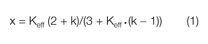
where k is the ratio K_H/K_L of the higher and lower relative permittivities of the two materials used, and K_eff is the mixture effective permittivity as measured in situ in the pipe. Note that if a particulate solid has been used for calibration, then the relative permittivity is that of the bulk material, not the pure solid. More sophisticated models are presented by Hunt, ¹⁰ but the Maxwell model is a fair approximation for many flows of near-spherical solids.

By cross-correlating pixels or groups of pixels between the first plane and a second axially separated plane, transit times and hence velocities can be measured.

Figure 6 shows an expanded section of the same data set as Figure 5 . The concentrations from the upper plane are shown as the green line and the lower plane as the red line for the gravity-drop flow of wheat through the sensor. It can be seen that despite the nominally uniform flow, there are significant flow ‘features’ which pass from upper to lower plane with a time delay of about 0.025 s. Since the separation between the two measurement planes is 0.05 m, then the downwards velocity of the wheat can be seen to be approximately 2 m/s. This velocity is calculated by cross-correlation of the concentration measurements from the two planes, and all flows of dispersed solids yet measured show sufficient flow structure for this to work successfully.

Figure 6.

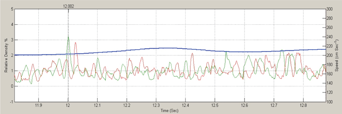
Concentration versus time for the flow of wheat in a 120-mm diameter pipe, data shown from the central zone of 13 for the same flow as shown in Figure 5 . The green line shows data from the upper plane against the left hand axis, the red line is from the lower plane, and the blue line is cross-correlation velocity shown against the right hand axis

The correlation process is described mathematically as

$$R_i(\tau )=\underset{T\to \infty }{\lim }\frac{1}{T}{\displaystyle \underset{0}{\overset{T}{\int }}{C}_{1,i}(t)C_{2,i}(t+\tau )dt}$$

(2)

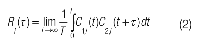
where C_1,i(t) and C_2,i(t) are the instantaneous concentrations in zone i in plane 1 and 2, respectively. Although mathematically the correlation is described for the averaging time T approaching infinity, in practice, the velocity will fluctuate over some much shorter time scale, and the user will need to set the window T at some suitable value appropriate to the particular length and velocity scales in the flow and the sensor geometry. The results here use an averaging window of 1 s.

The resulting correlogram (shown in Figure 7 ) has a clearly discernible peak if the flow structures are coherent over the sensor length and contains information about the time domain statistics of the flow – primarily convection and dispersion. The simplest assumption is that the time delay at the peak of the correlogram corresponds to the transit time of flow structures between the two planes. The peak may be found by the greatest single value, centre of area, or polynomial fitting. The time window used for the correlation process needs to be shaped in some way to minimise artefacts caused by sharp-edged windows. This shaping is known as apodization, and various apodization functions are used – the results presented here use the common Hanning window, which is a smooth bell shape.

Figure 7.

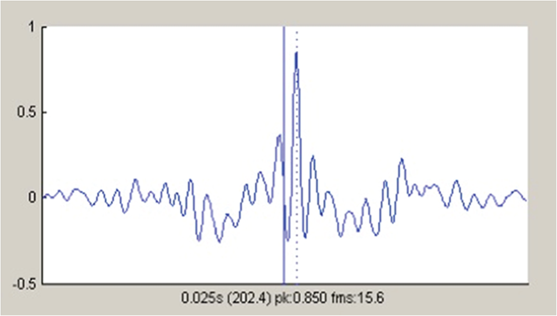
Cross-correlogram from the data shown in Figure 6 . Horizontal axis shows delay time; vertical axis shows correlation coefficient. The figures below the axis show delay time to the peak (0.025 s), equivalent velocity (202.4 cm/s), correlation coefficient at the peak (0.850), and number of frames of data equivalent to the peak delay time (15.6 frames)

If τ_i(t) is the time delay at the correlogram peak for zone i at each frame at time t, then the transit velocity is given by:

$$V_i(t)=S/{\tau }_i(t)$$

(3)

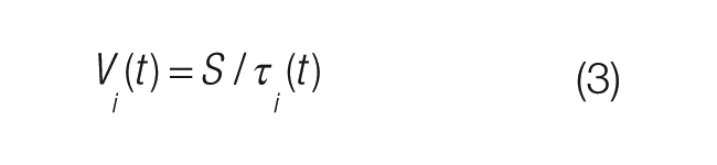
where S is the separation distance between the centre of the sensor electrode planes. The peak of the correlogram in the instance shown in Figure 7 is at a time delay of 0.025 s, corresponding to the average transit time of the solids between the two planes, and clearly seen on the concentration graph. The blue line on Figure 6 is this velocity calculated at each point in time, and referring to the right hand axis in cm/s.

By integrating over specified time periods around flow structures of interest, it is possible to measure the volume of individual large particles or clusters of particles, and by calibrating mass per unit length of the sensor, these measurements may be expressed directly as particle or cluster mass. ⁴

From these measurements in all 13 zones, we have the concentration and velocity in every part of the flow. The volumetric flow per zone is given by

$$q_i(t)=V_i(t)\cdot C_i(t)\cdot A_i\cdot \text{Δ}t$$

(4)

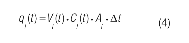
where Δt is the time interval between successive frames, and A_i is cross-sectional area of each zone. C_i(t) is in this case taken as the average of C_1,i(t) and C_2,i(t). The total volume flowing between time t₁ and t₂ can then be calculated as

$$Q={\displaystyle \sum _{t=t_1,t_2}}{\displaystyle \sum _{i=1,n}{q}_i(t)}$$

(5)

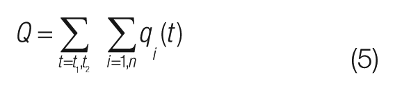
In many industrial situations, the required output is mass flowrate, which can be calculated by multiplying q by the average product density. In the case of dispersed solids, such as wheat, plastic beads, and wood pellets, the density is usually taken as the packed density measured at the same time as the reference material permittivity, thus minimising any errors due to estimates of packing density.

By comparing the integral of the flowrate over the length of a test, it is possible to compare the measurement of the total mass of product estimated by the ECT flowmeter and the weigh scale. Hunt ¹⁰ gives a summary of results for a selection of mill products and polyethylene terephthalate (PET) feedstock in a test rig with a 6-m drop showing that the uncertainty of measurement was typically between ±1% and ±3%.

In Figure 8 , we show typical results from repeatability tests of gravity-drop flows. In each test, 4 kg of wheat was released through the sensor from a hopper immediately above the sensor. For 20 repeat tests using the same material, the average deviation from the true mass was −0.4%, while the standard deviation of the errors was 1.0%. These figures are typical for such flows.

Figure 8.

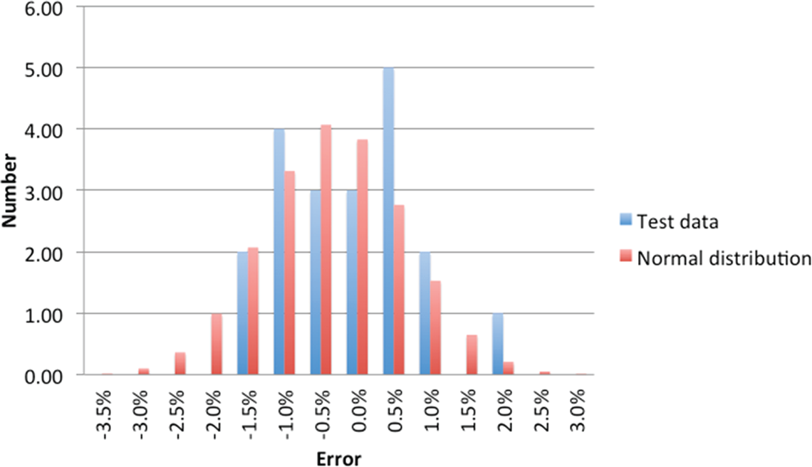
Error distribution for 20 repeats of 4 kg wheat in gravity-drop flow

Overall uncertainty of measurement for dry solids flows will also depend on other factors. The most important variations will come from product moisture content, process temperature, and particle shape. All of these factors may be corrected for if reference measurements are available.

V. Flow Structure Measurements

By creating zone maps which are more specific than that shown in Figure 3 , detailed information may be obtained about the flows, as well as simple overall flowrate measurements. Figure 9 shows a zone map where 16 of the zones are 2 × 2 pixel squares defining a diameter of the sensor, while the 17th zone is the remainder of the cross-section.

Figure 9.

Zone map used for the results shown in Figures 10 and 11

For each of the small zones along the diameter, the concentration and velocity of the product can be measured, giving a profile across the pipe. The concentration profile is shown in Figure 10 and the velocity profile in Figure 11 . Both figures are for the same flow shown in Figure 5 .

Figure 10.

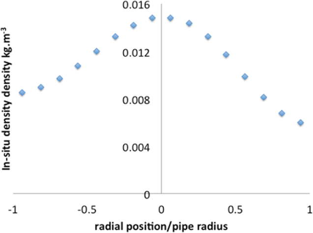
Concentration profile for wheat gravity-drop flow

Figure 11.

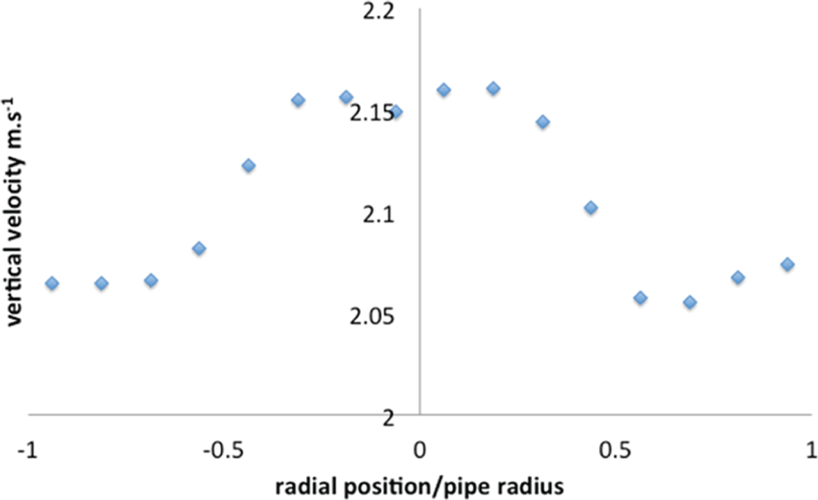
Velocity profile for wheat gravity-drop flow

In Figure 10 , the concentration is shown as in situ density – the mass of dry product per unit volume of the flow. Dry solids dropped under gravity typically tend to a distribution close to the wall of the pipe, as shown in Hunt, ¹⁰ but it can be seen in this case that the distribution is fairly symmetric. The flow passes through a distribution plate with a uniform array of 20-mm holes about 300 mm above the measurement location. Even with a forced uniform distribution so close to the sensor, the flow has already developed into the distribution shown.

The velocity profile ( Figure 11 ) also shows a centre peak, but the variation is quite small between 2.06 m/s near the wall and 2.16 m/s near the centre. In industrial situations, the distribution of flow may be important to the nature of the process, and ECT offers a chance to measure in situ density and velocity of the product without any intrusion into the flow.

VI. Conclusion

ECT has a well-established reputation as a research tool and has been used in a number of industrial applications including dry solids flows, gas–liquid flows, and wet gas flows. ECT can give detailed flow structure information that has been experimentally validated against other techniques.

In use as an integrated multiphase flowmeter, ECT in gravity-driven flows of dispersed solids can give overall uncertainty of measurement in the region of ±1% to ±3% of reading across a wide range of mass flowrates.

ECT-based flowmeters capable of being mass-produced and deployed into the commercial industrial environment are being developed, and prototypes are available, but none are yet in full-scale manufacture. Sensors of this type are being designed for applications in milling, power generation, and pneumatic transport. Commercial meters designed to give mass flow readings can also give the sort of detailed images and in situ concentration and velocity measurements shown here.