
Abstract
Interest in fault diagnosis of systems has grown significantly in recent years as modern control systems are becoming more complex and control algorithms more sophisticated. Research and development engineers very often face the challenge to find out what fault diagnosis methods exist and what are their main benefits. Classification of fault diagnosis methods is presented in this paper based in three main categories, namely, model-based, hardware-based and history-based fault diagnoses.
I. Introduction
Most of large-scale control systems are increasingly relied upon to provide product quality, safety and operational reliability for long periods of time. Most of these control systems are made from components which are subject to manufacturing defects, wear and tear, interactions with the environment and other causes of performance degradations. It is important, therefore, that control systems are able to diagnose and compensate for fault conditions regardless of their operational mode being online (i.e. chemical plants) or real time (i.e. automotive systems).
II. The Main Idea of Fault Diagnosis
The main idea of fault diagnosis is to determine the type, size and location of the fault as well as its time of detection, based on the available measurements of the system. A general scheme of model-based fault diagnosis is shown in Figure 1 . Usually, fault diagnosis is achieved in a two-stage process. First, a signal called residual is generated using available input–output measurements from the system under consideration. When the system is fault free, then residual should be zero or close to zero, and otherwise when the fault is present, residual should be different from zero. Residual could be scalar signal carrying information of a single fault or vector carrying information of multiple faults. The type of the residual generator varies from an analytical mathematical model to a black-box model of the system. The second stage is the decision-making process where residuals are examined for the likelihood of faults. The type of the decision-making mechanism varies from a simple threshold to a number of sophisticated statistical approaches.
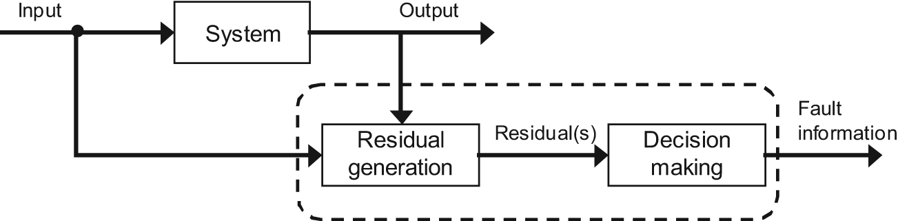
General scheme of model-based fault diagnosis
III. Types of Faults
Consider an open-loop dynamic system separated into three parts: actuator(s) plant dynamics and sensor(s) with input u(t) and measured output y(t) as depicted in Figure 2 . In fault diagnosis of dynamic systems, it is important to model all effects that can lead to alarms or false alarms. Faults can occur in the actuator(s), in the component(s) or parameter(s) of the plant dynamics and in the sensor(s). Modelling error(s) can be introduced between the actual system (actuators, plant dynamics and sensors) and its mathematical model. Finally, system noise (also called unknown input) and measurement noise should be taken into consideration to avoid triggering false alarms. The dynamic system shown in Figure 2 can be described using the continuous linear state Equations (1) and (2). Where x is the state vector, u is the input vector, y is the measured output vector, d is noise or unknown input vector, f is the fault vector and w is the modelling error vector. Term Ed models the unknown inputs to the actuator(s) and to the plant dynamics, Kf models the actuator and component(s) or parameter(s) faults and Rw models the modelling errors to the actuator(s) and to the plant dynamics. Term Fd models the unknown inputs to the sensor(s), Qf models the sensor(s) faults and Sw models the modelling errors to the sensor(s). A, B and C are the nominal system’s matrices since the faults that are principally reflected in changes of A, B and C are considered by d, f and w associated with proper choices of E, K, R, F, Q and S.
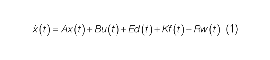
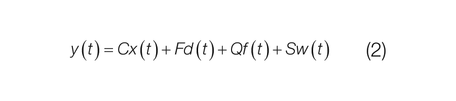
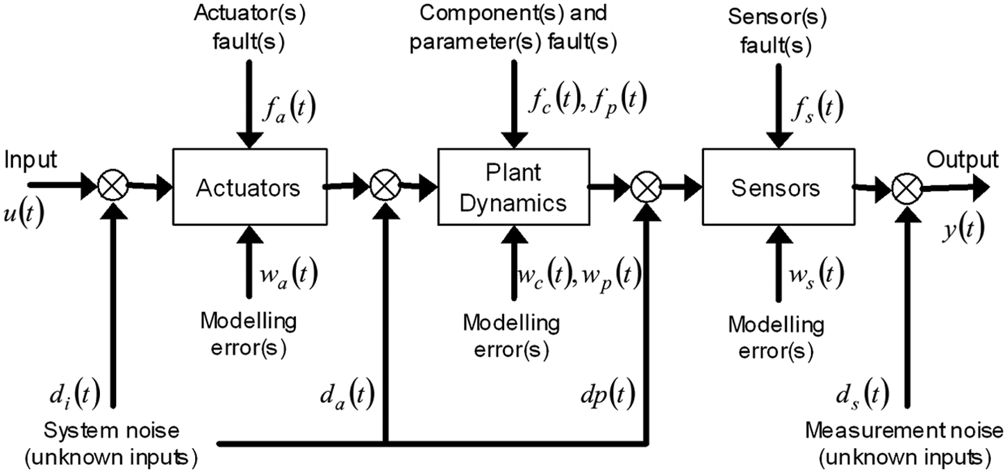
Modelling of open-loop faulty system
IV. Classification of Fault Diagnosis Methods
There is great quantity of literature on dynamic systems fault diagnosis ranging from analytical methods to artificial intelligence and statistical approaches. From a modelling prospective, there are methods that require accurate system models (plants), quantitative models or qualitative models. However, there are methods that do not require any form of model information and rely only on historic system data. While there have been some excellent reviews in the field of fault diagnosis, it is of interest that classification of fault diagnosis methods very often is not consistent. This is mainly due to the fact that researchers are often focused on a particular branch, such as analytical models, of the broad discipline of fault diagnosis. Classification of fault diagnosis methods is presented in this paper based on the contributions of various researchers.1–8 This classification of fault diagnosis methods is shown in Figure 3 . Fault diagnosis methods are broadly classified into three main categories: model-based, hardware-based and history-based. Each category is discussed briefly in the following sections.
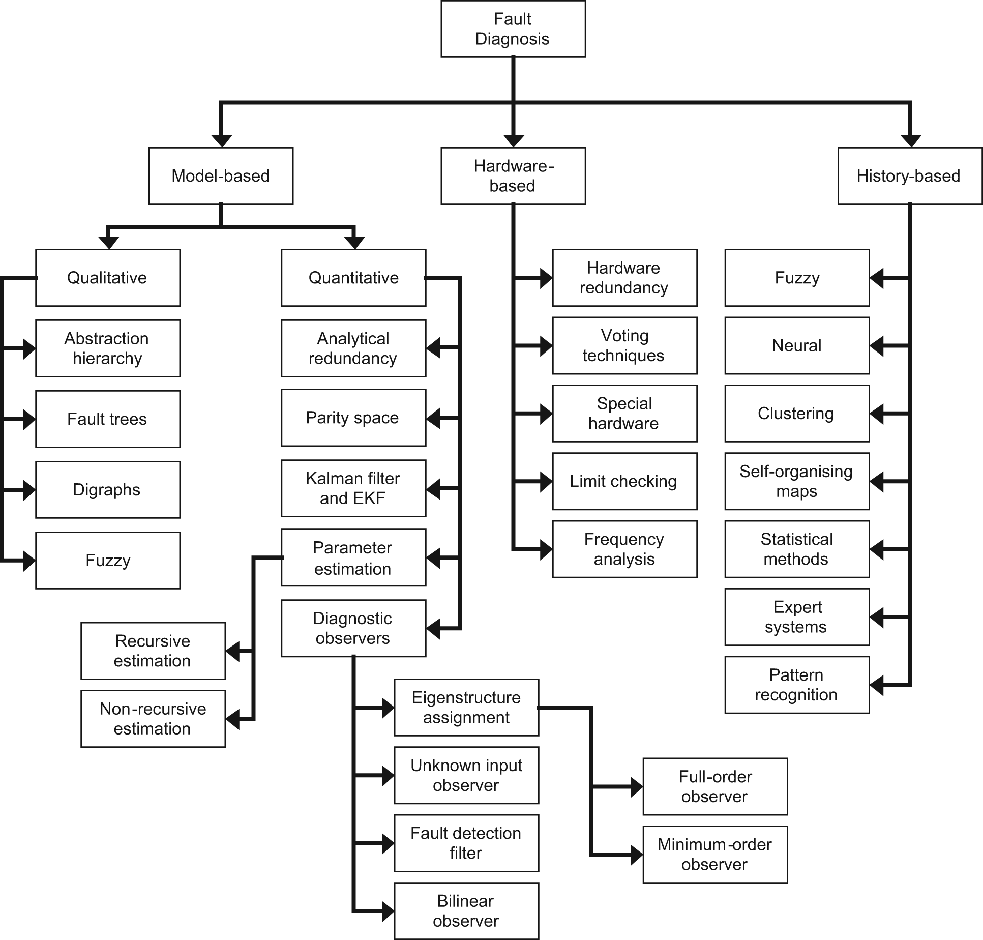
Classification of fault diagnosis methods
A. Model-Based Fault Diagnosis
Model-based fault diagnosis methods usually deploy a model developed based on some fundamental understanding of the physics of the plant or process. In general, model-based fault diagnosis methods are broadly classified as qualitative or quantitative.
Qualitative methods
Qualitative model-based fault diagnosis methods utilise a model where the input–output relationship of the plant is expressed in terms of qualitative functions cantered around different units in the process. Qualitative model-based fault diagnosis is broadly classified into abstraction hierarchy, fault trees, diagraphs and fuzzy systems.
(a) Abstraction hierarchy. Abstraction hierarchy is based on decomposition. The main idea behind decomposition is to draw inferences about the behaviour of the overall system based on the laws governing the behaviour of its subsystems. In control systems, these subsystems represent various individual control loops.
(b) Fault trees. Bell Telephone Laboratories developed the concept of fault tree analysis in 1961. A fault tree diagram follows a top-down structure and represents a graphical model of the pathways within a system that can lead to a foreseeable, undesirable loss event (or a failure). The pathways interconnect contributory events and conditions using standard logic symbols. The AND and OR symbols (gates) are the two most commonly used gates in a fault tree.
(c) Diagraph. Diagraph is a graph or set of nodes connected by edges, where the edges have a direction associated with them. Directed arcs lead from the ‘cause’ nodes to the ‘effect’ nodes. Each node in the signed diagraph corresponds to the deviation from the steady state of a variable.
(d) Fuzzy logic. Fuzzy logic (FL) is used in the field of fault diagnosis particularly those that are qualitative model-based and process history-based. Fuzzy logic systems (FLS) employ qualitative linguistic terms that take into account the imprecise nature of real-world processes and systems. FLS offer the following: they allow the handling of processes that are either modelled inadequately or not representable mathematically; they describe process behaviour based on available empirical or experiential information from sensors systems and/or human operators; they can cope with complex non-linear, multi-variable and time-varying processes without requiring them to be defined in precise mathematical terms.
B. Quantitative Methods
Quantitative model-based fault diagnosis methods utilise a model where the input–output relationship of the plant is expressed in terms of mathematical functions. As shown in Figure 3 , quantitative model-based fault diagnosis is broadly classified into analytical redundancy, rarity space, Kalman filter (KF), parameter estimation and diagnostic observers.
Analytical redundancy
Analytical redundancy makes use of mathematical model of the system under consideration. In the fault diagnosis literature, very often, analytical redundancy is referred to as model-based fault diagnosis. Using analytical redundancy, fault diagnosis is achieved by direct comparison between measured signals (from the actual system) and generated signals (estimated from a mathematical model of the process). As mentioned previously, the difference between the measured signals and the signals generated by the mathematical model form the residual. A diagnostic logic is used to assess this residual and therefore to decide whether an alarm signal should be flagged. A potential problem encountered using analytical redundancy is a false alarm rise due to poor mathematical model of the process, high system noise and modelling errors.
Parity space
The basic idea of parity-space approach is to provide a proper check of the parity (consistency) of the input–output measurements of the system under consideration. In theory, under steady-state operating conditions, the residual generated by the parity-space method is zero. However, the residual are non-zero due to input–output measurement and process noise, modelling errors and faults in the system.
KF
KF is used to design a state estimator with minimum estimation error. The prediction error of the KF can be used to form fault detection residual. In particular, the system is in a fault-free state if the residual has zero mean and non-zero if fault is present.
Parameter estimation
In some cases, a fault could occur due to changes in the system parameters (parameter fault
Diagnostic observers
In the fault diagnosis literature, one can find different types of diagnostic observers for residual generation. 1 The following are very common diagnostic observers for residual generation.
Residual generation using eigenstructure assignment. This observer decouples directly the generated residual from disturbance (disturbance may not be decoupled from state estimation).
Residual generation using unknown input observer (UIO). The main principle of the UIO is to make the state estimation error decoupled from the unknown inputs (disturbances).
Residual generation using fault detection filter. Fault detection filter is a full-state estimator with a special choice of the feedback gain matrix.
Residual generation using bilinear observer. A special class of non-linear systems can be treated using bilinear models or observers. There are two main approaches in designing bilinear observers for fault diagnosis; the first approach uses the Lyapunov method, whereas the second approach is based on the use of techniques developed for linear UIOs.
C. Hardware-Based Fault Diagnosis
Hardware-based fault diagnosis methods do not deploy a mathematical model of the physics of the plant or process. In general, hardware-based fault diagnosis methods are broadly classified into hardware redundancy, voting techniques, special hardware, limit checking and frequency analysis.
Hardware redundancy
Hardware redundancy is the traditional approach to fault diagnosis which uses multiple sensors and actuators in order to measure a particular variable of interest. A major setback with hardware redundancy is the extra equipment (sensors and actuators), extra weight and maintenance cost associated with them. Furthermore, the additional space required to accommodate the equipment makes hardware redundancy an unpopular method for fault diagnosis.
Voting techniques
Voting techniques are often used in systems incorporating a high degree of parallel hardware redundancy. Voting techniques are fairly easy to implement and mostly suited for fault diagnosis in instruments with mechanical faults. To describe how a voting technique will work, consider three identical sensors measuring the same variable. If one of the three signals differs distinctly from the other two, the differing signal is identified as faulty. The difference between the two signals in every pair of sensors in a redundant group indicates a fault.
Special hardware
Special hardware can be used specifically for fault diagnosis in dynamic systems. Special hardware is usually different types of sensors, used to measure quantities such as temperature, pressure, sound or vibration. Then, limit checking is performed to detect faults in the system under consideration.
Limit checking
Using limit checking, the process variables are measured and compared to known limit for each variable. Typically, the first step is to establish the variables threshold and then to compare them with the measured values. Any measurement or comparison between known threshold and measured value outside the expected range would indicate the presence of fault. A simple example is the case of a house smoke alarm where the alarm bell is triggered when smoke in the house has reached a predefined threshold.
Frequency analysis
Frequency analysis of plan measurements can be successfully used in fault diagnosis of dynamic systems. Most plant variables exhibit a typical frequency spectrum under normal operating conditions. Any deviation from this can be interpreted as abnormality. Certain types of faults may even have their characteristic signature in the spectrum, facilitating direct fault isolation.
D. History-Based Fault Diagnosis
In fault diagnosis literature, one can find a huge overlap between model-based fault diagnosis and history-based fault diagnosis. As previously mentioned, model-based fault diagnosis methods usually deploy a model developed based on some fundamental understanding of the physics of the plant or process. History-based fault diagnosis methods do not deploy a mathematical model of the physics of the plant or process, but a model derived from known and measured input and output process data. The fundamental idea of history-based fault diagnosis is to generate a model of the process, which mathematically relates measured inputs to measured outputs, and then use this model against the real process to generate residual. In general, history-based fault diagnosis methods are broadly classified into FL, neural networks, clustering, self-organising maps (SOM), statistical methods, experts systems and pattern recognition.
FL
The use of FL in the field of model-based fault diagnosis was mentioned previously. There FL used to derive a model of the system and then use it as an observer to generate residual. The main difference between usage of FL in model-based and history-based fault diagnosis is the type/method of fuzzy model/observer generation. In model-based fault diagnosis, the fuzzy model is generated having some knowledge of the system behaviour allowing the construction of the rule-base and selection of type and number of membership functions for each input/output variable. In history-based fault diagnosis, the fuzzy model is generated using observed input/output data. With input/output observation data, clustering techniques can be used to auto-generate a fuzzy model.
Neural networks
Artificial neural networks (ANN) are mostly suited for fault diagnosis of non-linear dynamic systems. ANN have interesting and attractive features such as learning, self-organisation and the capability to model a large class of non-linear systems. ANN can learn a mapping between an input and output space and form an associate memory that retrieves the appropriate output when presented with an unseen input. They can also generalise to produce an output when presented with previously unseen inputs. Calculations are in principle carried out in parallel resulting in speed advantages, and programming can be done by training rather than defining explicit instructions.
Clustering
Clustering can be an effective technique for dealing with large sets of data. The principal idea is to distil natural groupings of data from a large data set thereby allowing concise representation of the system’s behaviour. In fault diagnosis for dynamic system, clustering can be used to generate model to act as an observer for residual generation. This is the case where a fuzzy observer is considered to predict the system’s outputs.
SOM
SOM are special type of neural networks based on unsupervised learning. The main objective of SOM is to classify input vectors according to how they are grouped in the input space by learning both the distribution and topology of the input vectors they are trained on.
Statistical methods
Various statistical methods are used to develop the relationship between inputs and outputs of a system under consideration for fault diagnosis. Some examples of statistical methods include linear and multiple regression, polynomial regression, principal component analysis, partial least squares and logistics regression. These methods are usually referred to black-box statistical methods for fault diagnosis. Fault diagnosis is a classification problem and hence can be cast in a classical statistical pattern recognition framework.
Expert systems
Expert systems are computer-based applications used to deploy the insights, knowledge and/or guidance of individual with expertise in a given field. Usually, the main components in the expert system development include knowledge acquisition, choice of knowledge representation, the coding of knowledge in a knowledge base, the development of inference procedures for diagnostic reasoning and the development of input–output interfaces. Some of the advantages in the development of expert systems for diagnostic problem solving are ease of development, transparent reasoning, the ability to reason under uncertainty and the ability to provide explanations for the solutions provided. The main weaknesses are that they are very specific to a system, can miserably fail beyond the boundaries of the knowledge incorporated in them and are difficult to update or change.
Pattern recognition
In pattern recognition (or classification), one tries to assign a class label to an object, a physical process, or an event. Licence plate recognition is a good pattern recognition example. In a speeding detector, the sensors are a radar speed detector and a high-resolution camera, placed in a box beside a road. When the radar detects a car approaching at high velocity, the camera is signalled to acquire an image of the car. The system should be capable of recognising the licence plate, so that the driver of the car can be fined for the speeding violation. The system should also be robust to differences in car model, illumination and weather conditions. Fault detection of dynamic systems using pattern recognition is achieved incorporating a similar approach.
V. Conclusion
The aim of this paper was to present a classification of fault diagnosis methods and give very brief overview of each method. Because of the current tremendous research activity in this field, the paper has focused, on those methods, which are well established in the engineering and research community. In particular, fault diagnosis methods were classified into three main categories: model-based, hardware-based and history-based methods.
Model-based fault diagnosis methods have the following strengths: they provide the most accurate estimators or observers when they are well implemented, detailed models can model both normal and faulty operations of the system under consideration and system noise and modelling errors can be modelled and incorporated into fault diagnosis strategy. They also have the following weaknesses: mathematical models could be complex and therefore computationally intensive; modelling misjudgements could have significant impact on final results.
Hardware-based fault diagnosis methods have the following strengths: easy and cheap to implement, well recognised and trusted. They also have the following weaknesses: extra equipment associated with high maintenance cost and require additional space to accommodate the extra equipment.
History-based fault diagnosis methods have the following strengths: well suited for highly non-linear systems and do not require understanding of the physics of the system being modelled. They also have the following weaknesses: models cannot be used beyond the training data range, models are specific to the system being modelled and training data are required from both normal and faulty operations.
As a general conclusion, the question of suitability of any of the above fault diagnosis methods is primarily a question of the quality of the available mathematical model of the system, knowledge of the system and system structure. In addition to this, the reachable quality of fault isolation decisively depends on the number of available measurements.
Footnotes
Funding
This research received no specific grant from any funding agency in the public, commercial or not-for-profit sectors.