Online Use of the Fuzzy Transform in the Estimation of Electric Vehicle Range

Abstract

The phenomenon of range anxiety is a disincentive to the uptake of electric vehicles by a large proportion of drivers despite the range afforded by an electric vehicle being more than is required by the majority of drivers for their daily journeys. Although efforts continue to alleviate the situation through increasing the autonomous range of vehicles that operate from a battery, in some cases, it might be that range anxiety may also be mitigated through better driver information. However, the systems comprising any vehicle and an electric vehicle in particular are highly complex and nonlinear and do not lend themselves to analytical modelling to allow range prediction; instead, model-free methods must be employed. One relatively recent advance in model-free methods is the ‘Fuzzy Transform’, which has now been adapted to online use for the prediction of remaining range of an electric vehicle.

I. Introduction

A. The motivation: range anxiety

Range anxiety is a recent, but relatively well-known phenomenon, and is discussed widely in the press, other publications and media when electrical vehicles (EVs) are considered as a potential replacement for those equipped with an internal combustion engine.^1,2 Despite the fact that consumers drive approximately 53 km per day,^1,3,4 on average, the perception of consumers is that an EV must be able to provide a range of 473 km on a single charge (on average)¹ to be of use to them. This has rightly driven a large amount of development effort in the automotive industry and supply chain.

A recent study in Japan, however, has pointed out that factors outside the technologies that directly affect the range of an EV on a given journey may also provide the opportunity to increase the uptake of EVs in the marketplace. The study in question relates to a trial of EVs by the Tokyo Electric Power Company (TEPCO) in a local office.⁵ Part of the way through the trial, a fast-charging facility was introduced, but no other changes were made to the vehicles in use (i.e. their actual autonomous range on a single charge remained unaltered); the result was that use of the vehicles increased by over sevenfold in terms of distance travelled per month and over threefold in terms of the amount of charge used on any given journey, strangely though the fast-charging facility was rarely, if ever used. TEPCO believes that this is because the mere presence of the fast-charging facility gave a ‘psychological crutch’ to the staff using the EVs.

The work that is the subject of this article was based on a train of thought that began with that belief of TEPCO and led the authors to wonder what other means there might be of reassuring drivers, with the aim of increasing the use of EVs. It was hypothesised that better driver information in the form of a ‘range remaining display’ might be one such means and an investigation was then carried out into how this might be achieved.

B. The problem

Vehicles in motion are subject to nonlinear, time- and condition-varying relationships between energy used to overcome losses and speed.⁶ Since speed is the derivative with respect to time of distance, the expectation is that a nonlinear relationship also exists between the distance travelled and the energy used to travel that distance.

Furthermore, while they are continuous quantities, the state of charge (SOC) and velocity data captured in a vehicle using a means such as the controller area network (CAN) bus are both quantised and typically sampled at different rates. The non-deterministic nature of the CAN bus adds in variability to the spacing in time at which sequential samples of a given quantity are received; further noise is present in captured data, both in the underlying quantity and in the form of measurement noise.

Any means of establishing a relationship between energy used in propelling a vehicle and the distance travelled therefore needs to overcome these potential pitfalls. The Fuzzy Transform (F-transform) is proposed as being one component of such a means.

II. The Fuzzy Transform

The F-transform was first introduced in 2001,⁶ and a number of refinements^7
–9 and proposed refinements¹⁰ have been made to the method since that time. All of these original formulations were intended for offline use, but they also hinted at relatively simple changes that could be made to the method to also make it applicable to online use.

To those new to the method, the application of the offline form of the F-transform is perhaps initially best considered as being similar to the fast Fourier transform in that it is applied to a bounded window (of data) along a domain; to apply the method, one first takes a ‘fuzzy partition’ of this ‘universe’. The transform is then applied to the data within the partitions of the universe and introduces a mapping between the original space to a new special space; the inverse F-transform (iF-transform) then provides a reverse mapping that approximates the original function (with arbitrary precision). The new ‘fuzzy space’ into which the F-transform maps the original function allows the simplification of some operations through the ability to use methods of linear algebra in the fuzzy space, before mapping the solutions back to the real space via the iF-transform.

In the original (offline) forms, the F-transform has been used in the following areas and applications:

Numerical solution of ordinary differential equations, such as the Cauchy problem, including in situations where ‘traditional’ methods break down (e.g. with additive noise)^7,11

Approximation of the definite integral of the original data over the universe⁷

Data compression and image compression and reconstruction¹²

Removal of noise, image fusion and data analysis to determine dependencies between attributes¹³

Solution of partial differential equations (heat equation, wave equation and Poisson’s equation)¹⁰

Data series smoothing and interpolation¹⁴

Time series analysis and forecasting¹⁵

Generation of indicators for financial transaction decisions¹⁶

Based on the above list of uses, the F-transform was selected as part of a model-free approach to the estimation of the remaining range of an EV as its smoothing, compression and filtering properties were seen as particularly desirable in such an application:

The smoothing and filtering properties were deemed useful as they obviated the need for data processing to be performed on the inputs to the calculation process thereby lessening the computational requirements.

The compression property was deemed useful since this meant large quantities of input data could be ‘summarised’ using only a small amount of storage and then ‘reconstructed’ when required.

Various descriptions of the F-transform are available in the literature,^7–11 including one by the first author of this work that attempts to simplify some of the notation used.⁶

III. Using the F-transform Online

Because the F-transform operates on a universe (window of data), as new data points are found (through sampling), we need a way to cope with data outside the original universe. A trivial solution would be to discard all such data; however, the F-transform (when applied to a uniformly partitioned universe) lends itself to an ever-expanding universe, through the simple expedient of simply creating a new partition at the end of the universe.

At this point, it is worth noting that the F-transform allows the approximation of the function underlying the data with arbitrary accuracy,¹⁰ akin to the universal approximation capability of fuzzy sets.¹⁷ Taken in conjunction with the ability to add partitions to expand the universe, this leads to the question ‘how should the universe be partitioned?’ An analytical answer to this will be the subject of further work, but an heuristic found in the course of this work, based on empirical analysis of both moderately rapidly changing data (vehicle speed, sampled at 50 Hz) and less rapidly changing data (SOC, sampled at 10 Hz), is that sizing partitions to contain 200 samples gives an $R_{T}^{2}$ value of over 97.5% when comparing data that have been compressed and then reconstructed by the F-transform method to the original data.

Figure 1 shows an example of a uniform fuzzy partition of a universe (for a number of partitions of the universe, n = 9) with triangular membership functions $A_{j} (x)$ identified at each apex, equal partition widths, h_j, giving rise to evenly spaced nodes c_j at which the elements, F_j, of the n-tuple, F, describing the F-transform are calculated, along with an inset that shows how a partition may be referenced by a number ‘k’.

Figure 1.

Uniform fuzzy partition of an example universe with n = 9

It is worth noting that since the leftmost and rightmost data points in Figure 1 lie outside the universe, they will not be considered in any calculations of membership function values. Referring to the inset of Figure 1 , it may be seen that a given data point influences two elements of the n-tuple describing the F-transform, and this allows a simplification of the equations of the F-transform for the case of a uniform fuzzy partition of the universe.

The equations of the F-transform, adapted to online use, are then as given in Equations (1) to (4).⁶

n u m_{k, i} = n u m_{k, i - 1} + y_{i} A_{k} (x_{i})

(1)

n u m_{k + 1, i} = n u m_{k + 1, i - 1} + y_{i} (1 - A_{k} (x_{i}))

(2)

d e n_{k, i} = d e n_{k, i - 1} + A_{k} (x_{i})

(3)

d e n_{k + 1, i} = d e n_{k + 1, i - 1} + 1 - A_{k} (x_{i})

(4)

where num_j,i and den_j,i are the numerator and denominator, respectively, of the jth element of the F-transform that relate to the partition where the data point value, y_i, is captured at sample point, x_i. This formulation reduces computational load through only requiring one membership function value to be calculated for each data point.

Since the iF-transform is only used when the data stored by the F-transform are required, typically at a much lower frequency than data that enter the calculation, the original formulation of the iF-transform is used. The equation of the iF-transform thus remains as shown in Equation (5)^6–10,11

\begin{array}{l} f_{F, n} (x) = \sum_{k = 1}^{n} F_{k} A_{k} (x) \end{array}

(5)

where f_F,n(x) is the result of the iF-transform. Since this may be considered an estimate of the value of the function y = f(x) giving rise to the data points in the universe, we will adopt the notation $\hat{y} = f_{F, n} (x)$ for simplicity.^10,6

Due to the way the F-transform operates across two elements of the n-tuple when each data point is uncovered (as previously described), it is important that the iF-transform is performed only once the calculation of the n-tuple has moved on sufficiently that no further changes are required to be made to the elements corresponding to the nodes that bound the partition of interest. This results in a lag in calculations that may make the F-transform unsuited to direct use in real-time control applications; however, it remains useful as a method of extracting trends in data that may be used to adjust control strategies, or for parameter estimation tasks, where a degree of imprecision or delay may be tolerated.

Determination of which partition the estimator is operating within is then monitored by checking the truth value of the inequality x_i ≤ c_k + h; as soon as this becomes false, the sample point has moved into the next partition.⁶

IV. The Estimation of Remaining Range

The finalised method of range estimation then uses the F-transform to perform a transformation of time-varying vehicle speed, v, and SOC into a single distance-varying quantity. This is then used as the input to a parallel pair of recursive least squares (RLS) estimators, based on an assumption of a linear distance–SOC relationship to estimate the point at which the SOC, Q, will attain some final value; the combination of a ‘long-term prediction’ using all data points and a ‘short-term prediction’ using only recent data points aims to overcome any nonlinearity present in the relationship.

Taking the RLS parameter estimates of slope and offset and rearranging provides an estimate of the total distance that may be achieved in the entire journey, and a simple deduction of the distance travelled thus far provides the remaining range, the only remaining task being to apply some filtering at the output to slow transitions in the range remaining estimate when a new total distance travelled estimate is performed. A graphical representation of the calculation is provided in Figure 2 where the subscript k denotes the sample instant, x denotes the distance travelled and r denotes the range remaining.

Figure 2.

Graphical representation of range estimation calculation

Because the data for SOC and velocity both arrive at different intervals and sample times, the F-transform is used to interpolate (and resample) the SOC to match certain distance ‘tick-marks’. The distance tick-marks are found through integrating the incoming velocity data and interpolating based on an assumption of a linear time–speed relationship between sample points, to find the time at which a tick-mark was passed.⁶

The corresponding ‘tick-times’ found in this manner are then stored in a first-in first-out (FIFO) buffer along with the distance tick-mark values for processing to be carried out to find the corresponding estimated SOC value once time has moved on sufficiently as shown in Figure 3 .⁶

Figure 3.

Data transformation routine

V. Results

The method was implemented in the CANoe software published by Vector Informatik GmbH to allow replay of data captured from a 5.5 t Modec truck’s CAN bus and was compared with a reference method disclosed in a patent using the same data.¹⁸ Figure 4 provides screenshots of the graphics window of the CANoe software providing both the inputs to the system along with outputs; from top to bottom, the traces are velocity (in km h⁻¹), depth of discharge (transmitted by the battery and equal to 100% – SOC), range remaining (km) and distance travelled (km).

Figure 4.

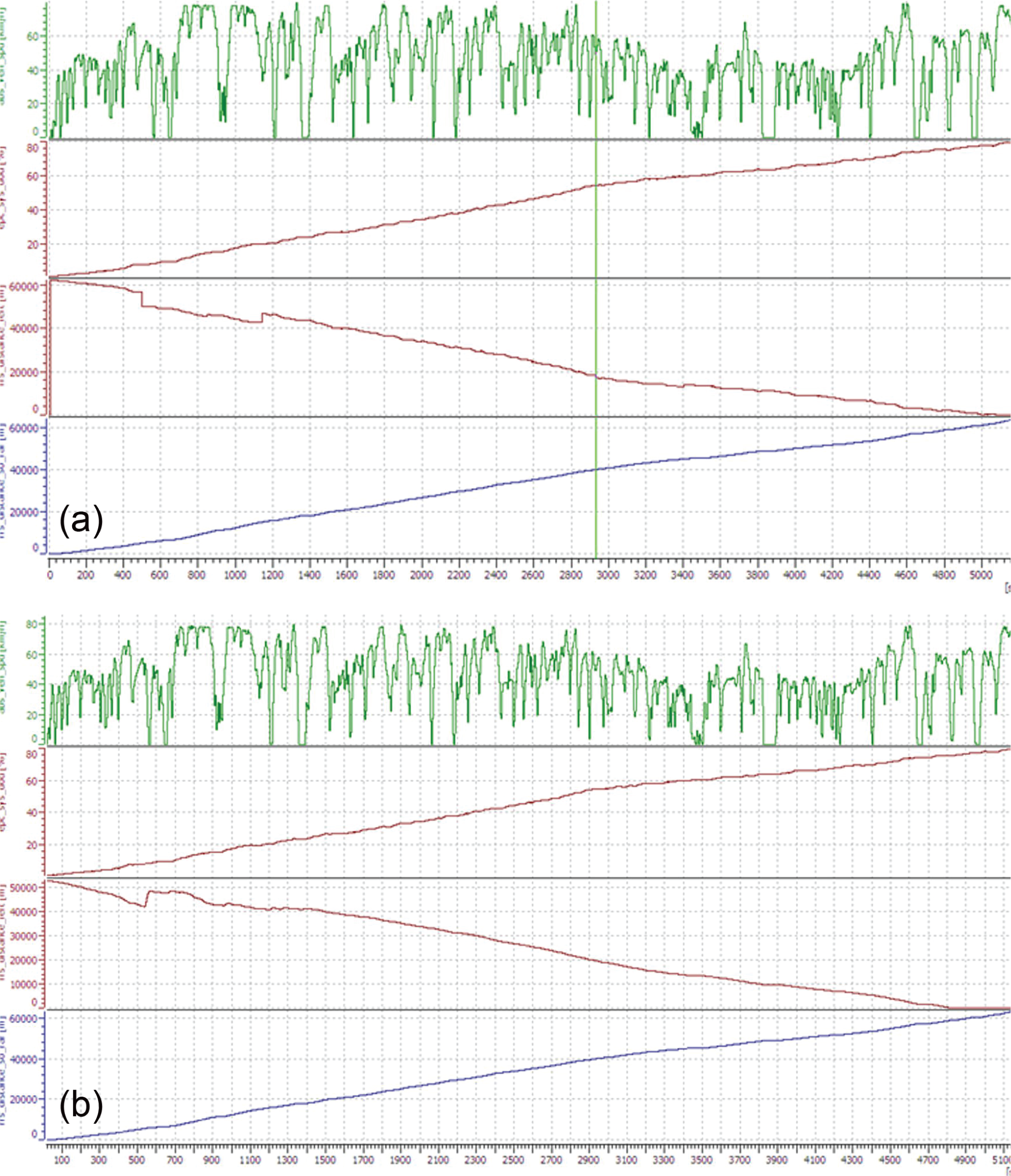
Results of (a) reference method and (b) F-transform method

From Figure 4 , it may be seen that the reference method gives rise to some large steps in predicted range remaining at approximately 500 s and 1150 s, along with smaller steps later, for example, at the location of the lime green cursor and again at 3400 s.

The F-transform method also has a small discontinuity, albeit more damped, at 550 s, marking the transition from an initialisation method that runs while sufficient data are gathered for the F-transform method to begin working (this initialisation phase uses an exponentially weighted moving average of ‘worst-case’ energy consumption and raw SOC). Work on the tuning of the initialisation phase or the switchover between the two methods is expected to be possible to minimise this transient.

The F-transform method was designed to deliberately ‘under-read’ by at least 1.5 km to give a conservative estimation, and this explains the short period of replay at the end where the provided range remaining value is zero, although further driving was possible. This behaviour is analogous to the fuel gauge in a vehicle fitted with an internal combustion engine where a short period of driving after the gauge reads ‘empty’ is usually possible (albeit not necessarily advisable!).

Some small upward perturbations are also visible in the results of the F-transform method from 600 s to 1200 s, and this is due to the RLS estimators not having converged fully; it is believed that tuning the estimators further (or changing to another estimator, such as the Kalman filter) would remove these through fast convergence.

It is believed that the smoother transitions of the F-transform method would be more acceptable to vehicle users and also prove less distracting to drivers than a value that undergoes rapid transitions.

In examining the underlying data of SOC and distance travelled, a curious relationship was observed in that the two quantities appear to be linearly related, in contradiction of the expectation that such a relationship would be nonlinear. Understanding this will be the subject of further work.

VI. Conclusion

The F-transform has been demonstrated in an incremental form that is suited to online use. This online form retains all the properties of the original formulation of the F-transform, while minimising computational needs. Through being recast into this online form, the F-transform is able to be used alongside more well-known control engineering techniques of signal processing and parameter estimation.

The online use of the F-transform was demonstrated in the estimation of remaining range of an EV. This prediction problem, although expected to be highly nonlinear in nature, turned out to be approximately linear. It is not clear whether this linearity was arrived at through recasting the problem into a spatial form, or whether the system itself does not exhibit the nonlinearity to the degree that was initially expected. If the linearity has resulted from the recasting of the problem into a spatial (rather than temporal) form, this may be of significant interest in further work.

Since carrying out the work reported herein, the authors have become aware of anecdotal evidence that points to the linearity being present in other sizes of EVs (including an electrically propelled ‘superbike’-class motorcycle).

Footnotes

Acknowledgements

The authors would like to thank Liberty Electric Cars for the provision of tools and data that enabled this work. Thanks are also given to Mr Joseph Mahtani and Professor Keith Burnham of Coventry University in the United Kingdom for their support and guidance throughout the work and Professor Irena Perfilieva of the Institute for Research and Applications of Fuzzy Modelling at the University of Ostrava in the Czech Republic for her responses to emails that enabled the scope of this project to be set. Finally, the authors extend their thanks to the reviewers for their time and valuable suggestions in preparing this work for publication.

Funding

This research received no specific grant from any funding agency in the public, commercial or not-for-profit sectors.

References

Accenture. Plug-In Electric Vehicles: Changing Perceptions, Hedging Bets. New York: Accenture, 2011.

Ralston

Nigro

Plug-In Electric Vehicles: Literature Review. Arlington, VA: Pew Centre on Global Climate Change, 2011.

Kintner-Meyer

Schneider

Pratt

Impacts assessment of plug-in hybrid vehicles on electric utilities and regional US power grids: part 1: technical analysis. Online Journal of EUEC 2007; 1: 1–39.

Massachusetts Institute of Technology. The electrification of the transportation system: issues and opportunities. In Symposium, Massachusetts Institute of Technology, Cambridge, MA, 8 April 2010.

Aoki

The Standardization of Electric Mobility towards CO₂ Reduction. Tokyo, India: The Tokyo Electric Power Company, Inc., 2010.

Cunningham

Application of the fuzzy-transform to estimation of the remaining range of an electric vehicle. Control Theory and Applications Centre, Coventry University, Coventry, 2012, Master’s Thesis.

Perfilieva

Fuzzy transforms. In Transactions on Rough Sets II, vol. 3135. Berlin/Heidelberg: Springer, 2005, pp. 391–430.

Štĕpnička

Fuzzy transform and its applications to problems in engineering practice. Department of Mathematics, University of Ostrava, Ostrava, 2007, PhD Thesis.

Perfilieva

Fuzzy transforms: Theory and applications. Fuzzy Sets and Systems 2006; 157(8): 993–1023.

10.

Stefanini

F-transform with parametric generalized fuzzy partitions. Fuzzy Sets and Systems 2011; 180(1): 98–120.

11.

Perfilieva

Haldeeva

Fuzzy transformation. In Proceedings of the joint 9th IFSA world congress and 20th NAFIPS international conference, 2001, vol. 4. New York: IEEE, 2001, pp. 1946–8.

12.

Perfilieva

Fuzzy transforms: A challenge to conventional transforms. In Hawkes

(ed.) Advances in Imaging and Electron Physics, vol. 147. Amsterdam: Elsevier, 2007, pp. 137–96.

13.

Perfilieva

F-transforms – Where fuzzy and classical mathematics meet. Applied and Computational Mathematics 2011; 10(1): 122–32.

14.

Štĕpnička

Dvořák

Pavliska

Vavříčková

A linguistic approach to time series modeling with the help of F-transform. Fuzzy Sets and Systems 2011; 180(1): 164–84.

15.

Di Martino

Loia

Sessa

. Fuzzy transforms method in prediction data analysis. Fuzzy Sets and Systems 2011; 180(1): 146–63.

16.

Troiano

Kriplani

Supporting trading strategies by inverse fuzzy transform. Fuzzy Sets and Systems 2011; 180(1): 121–45.

17.

Nguyen

Walker

EA.

A First Course in Fuzzy Logic. 3rd ed. Boca Raton, FL: Chapman & Hall/CRC, 2006, pp. 242–5.

18.

Grider

Blakemore

BC.

System and Method for Determining an Expected Vehicle Drive Range (US Patent Application Number US 2011/0166810 A1). Alexandria, GA: United States Patent and Trademark Office, 2011.