Use of Confidence Limits to Set Robust On-Board Diagnostic Thresholds

Abstract

Vehicles sold in the United States and Europe are equipped with a specific set of legal diagnostics, called on-board diagnostics; these are used to monitor the performance of various elements of the emission control system. The driver is informed of any failures by the use of a Check Engine Light on the dashboard of the vehicle and then should return the vehicle to the dealership for rectification. The vehicle manufacturer’s aim is to ensure that the Check Engine Light is only illuminated for legitimate failures. For the calibration of an on-board diagnostics, there needs to be sufficient separation between the response of a good sensor and a failed sensor; the setting of this threshold should be based upon a statistical model of the data so that the predicted failures rate can then be determined. An additional benefit of obtaining a statistical model is that it allows confidence limits to be applied to the data; this then gives the engineer the ability to determine the trade-off between the number of data points and the confidence in the estimated statistical model.

I. Introduction

Vehicles sold throughout the world are subject to an increasingly stringent set of emission thresholds. To achieve certification, all sensors and vehicle subsystems that may affect vehicle exhaust emissions have to be monitored by an on-board diagnostics (OBD) system that is part of the engine management system (EMS) or any other embedded controller. ¹ This requirement was first introduced in the United States in 1988 for OBD1, for open- and short-circuit faults, and in 1994 for OBD2, for changes in sensor and actuator responses. ² For Europe, this legislation, denoted European on-board diagnostics (EOBD), has been introduced for all vehicles built after January 2000. ³ Both sets of legislation link the performance of the different diagnostics to emission thresholds. In the event of component or subsystem failure, a ‘Check Engine’ Light must be illuminated as an indication to a driver that there is a problem, so corrective action can be taken to minimise the pollution caused by such a fault. As the emissions thresholds are continually reduced, more sophisticated techniques are required to be employed to meet these increasingly tightening thresholds.

As the Vehicle Emission Legislation drives down vehicle pollution, the impact on the diagnostics is that they have had to become increasingly more complex to determine a failed system. As a consequence, the diagnostics are becoming increasingly more complex, and with the resulting diagnostics, more likely to be models of the functions that they are monitoring, if only over a restricted set of operating conditions. As such, the residual error between the diagnostic output and the actual system response is more likely to fit to a Gaussian distribution.

OBD diagnostic calibration engineers develop test plans that invoke the worst case conditions for the diagnostics, by introduction of a variety of test conditions. These are typically different fuel specifications, operations at different ambient conditions (hot, cold and altitude), with different driving styles and tolerance sensors. Each diagnostic will have a set of worst case test conditions that have been developed through the experience of the engineer and lessons learnt. The approach used by the calibration engineer is to collect data for these conditions and then fit a Gaussian distribution to the data to set thresholds to ensure that a ‘normal’ system does not false flag and that a ‘failed’ system flag is detected in a timely manner.

By making use of Gaussian models and the use of confidence intervals, these models allow a more conservative and robust threshold to be set. Since the variation in the models reduces as more data are collected, they also provide the engineers with a way of gauging whether collecting any more data will significantly change their results. This is especially useful when collecting fault condition data where it is difficult to generate a large amount of data either because it requires specialist hardware setup or a specific environmental condition; usually, this is all against strictly limited project timing.

The article is organised as follows: Section II outlines the diagnostic used within this article, Section III outlines the set of conditions for setting the diagnostic thresholds, Section IV defines the calculation of the confidence interval, Section V details the implementation and analysis, and finally, Section VI details further work and concludes the article.

II. Problem Formulation

In modern engines, the air–fuel ratio (AFR) has to be tightly controlled so that the three-way catalyst is operating at its optimum conversion efficiency to provide the least amount of emissions. ⁴ AFR is measured as the ratio between the mass of air and the mass of fuel; for pure octane, the stoichiometric mixture is approximately 14.7:1. The exact composition of fuels varies seasonally and geographically; therefore, modern engines use a more convenient measure of lambda (λ) rather than AFR to allow them to control combustion process. A λ of 1.0 is at stoichiometry; rich mixtures are less than 1.0, and lean mixtures are greater than 1.0.

In this article, the calibration of an individual-cylinder air–fuel ratio diagnostic is investigated. This is a diagnostic which was first introduced for vehicles sold as 2010 Model Year vehicles.^5,6 Since this is still a relatively new diagnostic, it was decided to carry out a more detailed analysis of the diagnostic results. The data analysed in this article were collected from a cold ambient environment trip, this condition being deemed as being the worst case condition, potentially giving the smallest separation between the fault-free and the failed set of data.

Prior to the test trip, the failure condition for both a rich and lean shift in λ for individual cylinders was determined by carrying out tests over an emissions drive cycle, the point of failure being determined by the introduction of fuelling shift on to each cylinder in turn and determining the point at which the emissions result exceeds 1.5 times the certified emissions standard. ² The diagnostic will then generate an estimate of the λ shift that the closed-loop AFR control algorithm is generating, and this is then used to determine whether a fault condition has been reached.

III. Diagnostic Threshold Requirements

For this diagnostic, data need to be collected and analysed for three different distributions/conditions, the first condition being for a normal set of data; this is data where no additional fuelling shift has been added to the system. The other two sets of data will be for the rich and lean fuelling fault condition with their distributions lying to the left- and the right-hand sides, respectively, of the fault-free data distribution with a suitable gap between the tails of the fault and the fault-free sets of data.

Ideally, the fault threshold of the diagnostic should be set so that it captures all of the possible fault conditions. However, in practice, this may not always be possible; therefore, a minimum target of the detection of 90% of the fault conditions should result in the diagnostic bringing on the Check Engine Light. In the United States, the Check Engine Light is illuminated on the detection of two successive diagnostic operations. ² Therefore, to achieve the 90% detection on two successive tests requires that for a single test, the failure threshold should be set at a level that is approximately 95% (100√0.9). To determine the failure thresholds in the ‘Confidence Interval Calculation’ section, it is more convenient to convert this figure into a standard deviation. In this case, we are assuming that the threshold will only occur on one side of the distribution closest to the fault-free set of data. On the failure threshold side of the distribution, the point at which 45% of the population is represented by a standard deviation of 1.64, the other 50% of the failure data being containing in the other half of the distribution.

For the fault-free set of data, we need to ensure that the fault thresholds are greater than 3 × standard deviations from either side of the distribution. We will refer to this as the rich or lean robustness threshold. This will then allow 99.74% of the data to be correctly identified as being fault-free for a single diagnostic result. For the two successive diagnostic results, this would then lead to the possibility of flagging a fault-free system as having a fault of 1 in 148,000 tests.

IV. Confidence Interval Calculation

The set of data collected from the diagnostic cannot precisely define the characteristics of the population. The sample can only define a range of values for both the probable mean position and the probable standard deviation value. Confidence interval calculations are used to define a probable range of values for the population mean ${\overline{x}}_U$ (upper) and ${\overline{x}}_L$ (lower) and the population standard deviation ${\sigma }_U$ and ${\sigma }_L$ . This then generates a range of possible statistical models that will include the population model with a given confidence.

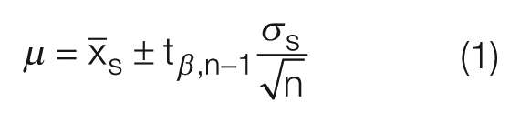
Equation (1) ⁷ is used to calculate the confidence interval for the mean

$$\mu ={\overline{x}}_s\pm t_{\beta ,n-1}\frac{{\sigma }_s}{\sqrt{n}}$$

(1)

${\overline{x}}_s$ is the sample mean, t is the confidence factor based on the Student’s t-distribution, ${\sigma }_s$ is the sample standard deviation, n is the sample size and β is either α for a single-sided confidence interval or α/2 for two-sided confidence interval, where α is the significance level, and for this article, a value of 5% or 0.05 will be used.

Calculation of the confidence limit for standard deviation is given by

$$\begin{array}{l}\text{lower}\text{limit}\text{upper}\text{limit}\hfill \\ {\sigma }_s\sqrt{\frac{n-1}{{\chi }_{\beta ,n-1}^2}}\le \sigma \le {\sigma }_s\sqrt{\frac{n-1}{{\chi }_{1-\beta ,n-1}^2}}\hfill \end{array}$$

(2)

${\chi }^2$ is the confidence factor based upon the chi-squared distribution.

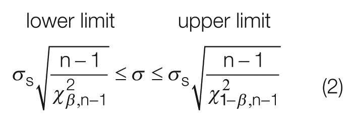
The results of equations (1) and (2) will produce a range of standard deviation and mean values which will include the population model with a 95% confidence. This confidence increases and the range of these values reduces as there is an increase in the amount of data, n, as it is collected. Using this range of values, it is then possible to choose a combination which will give the worst case failure or robustness thresholds. In terms of the standard deviation, it is the lower limit calculation in equation (2), ${\sigma }_L$ , which produces the maximum value of sigma, and this will generate a model which produces a greater range of λ values. The means, ${\overline{x}}_L$ or ${\overline{x}}_U$ , are chosen so as to give the smallest separation between the failure threshold and fault-free condition in each case.

V. Process Monitoring and Analysis

From testing, three specific sets of data were collected: a the fault-free set of data, represented by underscore F; a set of data in which a rich shift has been introduced to represent the emission failure threshold, represented by an underscore R; and a set of data for the lean shift, represented by an underscore L. This resulted in 6294 sets of results with a normal engine, 102 diagnostic results for the rich shift and 106 results for the lean shift.

The first thing to check is that all of the data sets have a Gaussian distribution. This was done using the LillieTest function within MATLAB, which performs a Lilliefors test^8,9 of the default null hypothesis to check whether the sample comes from a Gaussian distribution against the alternative that it does not come from a Gaussian distribution. The test returns a 1 if it rejects the null hypothesis at a significance level of 5%. For the fault-free condition, the set of data failed this test. For further investigation, these data are plotted on a quartile–quartile (QQ) plot. This plot shows the raw data as blue crosses plotted against an ideal Gaussian model, which is represented by the red dashed line. This shows that the bulk of the data, between the 5% and 95% percentiles, fits a Gaussian distribution. It is only the tail information of the distribution which does not match this statistical model. The shape of the tails in Figure 1 indicates that the data have come from a ‘fat tailed distribution’ where the data extend further than expected for the tails of a Gaussian distribution. This can be further seen by considering the 0.999 and the 0.001 percentile points which lie at points 0.925 and 1.07, respectively, and should, for a Gaussian distribution, lie at 0.94 and 1.06. Even though this statistical model does not accurately fit the data, it was decided to assume that the fault-free set of data could be considered to be Gaussian initially and then reviewed when the final thresholds for the rich and lean sides of the distribution have been determined. The risk in using this assumption is that the variance used for the fault-free data will be an underestimate of the true risk.

Figure 1.

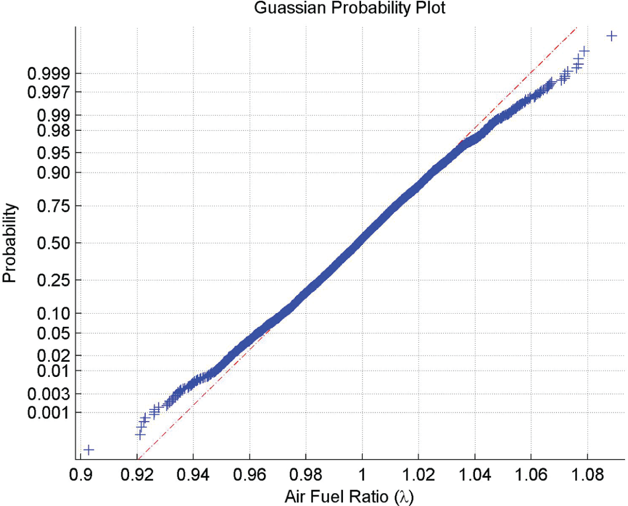
QQ plot for the fault-free data

Table 1 has been calculated for β = α/2 = 0.025 in equations (1) and (2). The standard deviation ${\sigma }_{L_F}$ , from Table 1, gives the largest value of sigma and is used to calculate the robustness threshold for both the rich and lean sides of the distribution. For the lean robustness threshold, the mean ${\overline{x}}_{U_F}$ was used to give a value of 1.0640; the rich robustness threshold was obtained using ${\overline{x}}_{L_F}$ which gives a value of 0.9330.

Table 1.

Statistical model for fault-free data (β = 0.025)

	LF	SF	UF
$\overline{x}$	0.9980	0.9985	0.9990
σ	0.0217	0.0213	0.0209

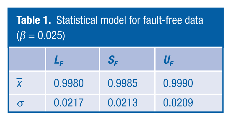
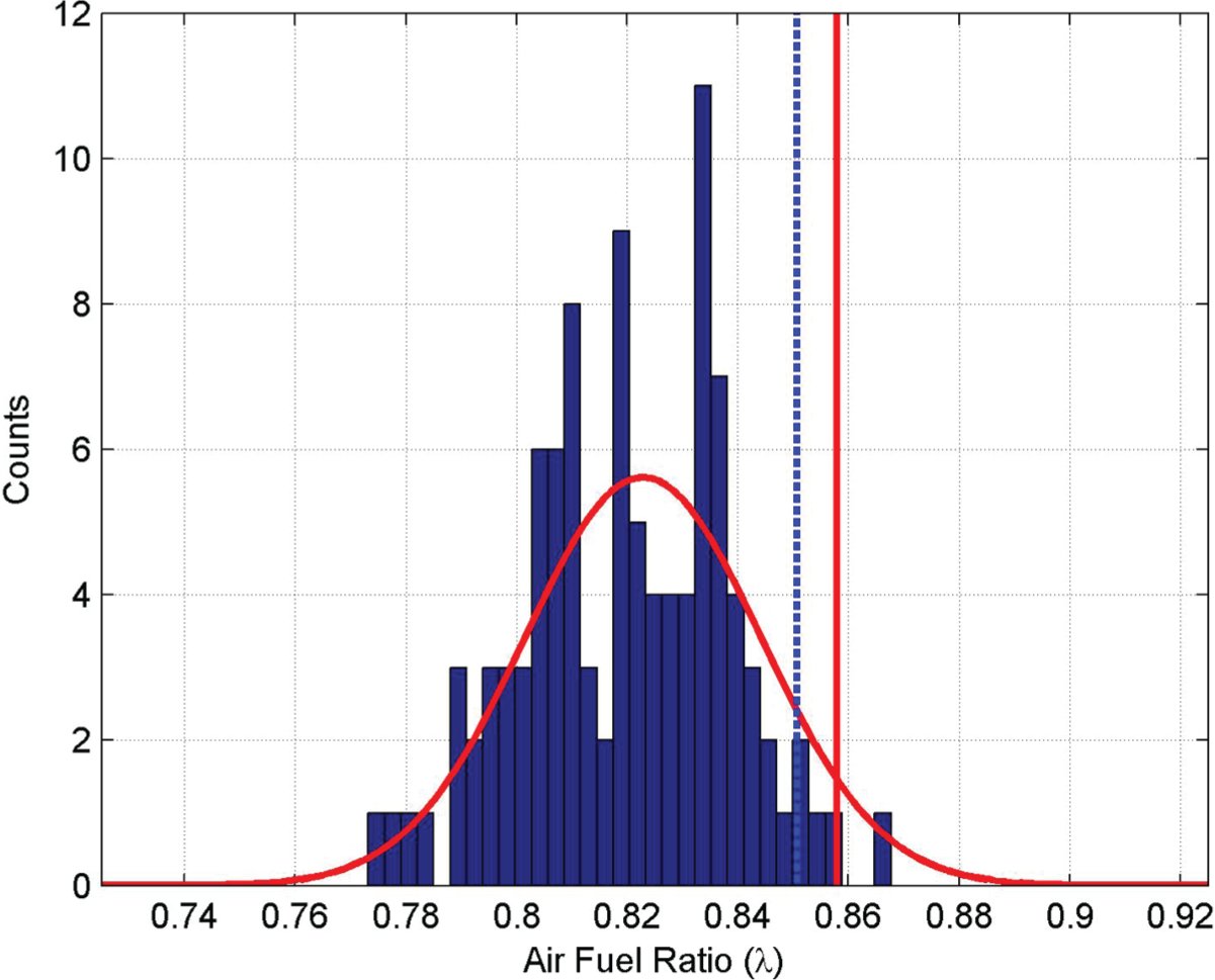
Table 2 shows the rich failure model information. It should be noted that since we are considering a single-sided threshold, β = 0.05. Figure 2 shows the histogram of the raw rich failure data, and the red solid line shows the worst case statistical model using ${\overline{x}}_{U_R}$ and ${\sigma }_{\mathrm{LR}}$ . Using this model, the rich failure threshold is calculated as 0.8579 and is shown on the graph by the solid vertical red line. The dotted blue vertical line shows the sample rich failure threshold of 0.8507 calculated by making use of ${\sigma }_{SR}$ and ${\overline{x}}_{SR}$ .

Table 2.

Statistical model for rich failure data (β = 0.05)

	LR	SR	UR
$\overline{x}$	0.8166	0.8197	0.8229
σ	0.0214	0.0189	0.0170

Figure 2.

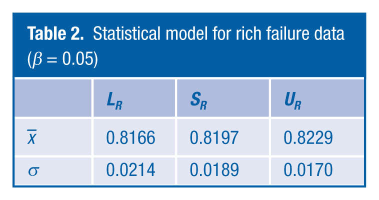
Statistical results for rich failure data

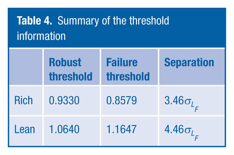
Since we are most concerned with the issue of falsely flagging a fault-free system, it is useful to take the difference between the rich failure threshold at 0.8579 and the rich robustness threshold at 0.9330 and then determine the amount of sigma separation between them. This difference is normalised by dividing by ${\sigma }_{L_F}$ to determine the amount of separation in terms of a sigma value and results in a separation of $3.46{\sigma }_{L_F}$ .

This then provides a clear robust threshold in terms of detection which meets the requirements and provides a significant safety margin against falsely flagging, and we have also taken into consideration the variability in the models by making use of the confidence interval.

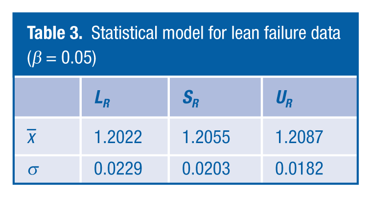
Figure 3 shows the response after introducing a lean failure shift. Again the graph shows the histogram of the raw data, and the solid red line shows the distribution of the worst case statistic model derived from ${\overline{x}}_{L_L}$ and ${\sigma }_{L_L}$ in Table 3 . The red vertical line shows the lean failure threshold of 1.1647 from this model and the dotted blue vertical line at 1.1723 for that derived from ${\sigma }_{SL}$ and ${\overline{x}}_{SL}$ . Using the same metric as previously derived, the difference between the lean failure threshold and the lean robustness threshold gives a separation of $4.64{\sigma }_{L_F}$ .

Figure 3.

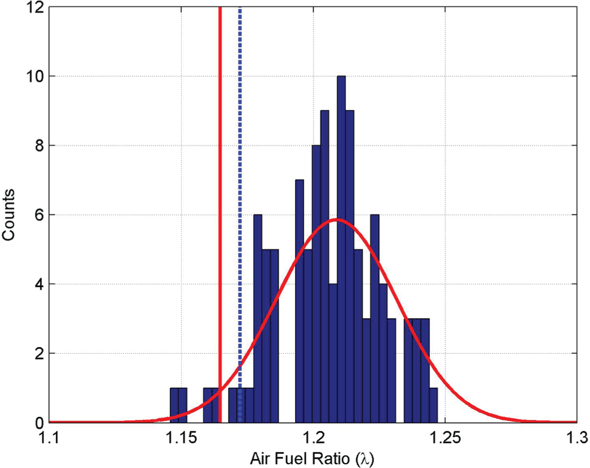
Statistical results for lean failure data

Table 3.

Statistical model for lean failure data (β = 0.05)

	LR	SR	UR
$\overline{x}$	1.2022	1.2055	1.2087
σ	0.0229	0.0203	0.0182

From the earlier discussion in the article, it has been highlighted that it can be difficult to collect fault condition data; therefore, it is useful to be able to assess whether enough data have been collected to ensure that the real distribution of the fault condition has been captured. To determine this, we have to make the assumption that the sample model information that we have is the best estimate of the distribution model. Therefore, in the rich failure case, the sample values of ${\sigma }_{SR}$ and ${\overline{x}}_{SR}$ from Table 2 have been used, and the value of n and the subsequent changes made to the t-distribution and chi-squared tests, in equations (1) and (2), can then be used to determine the effect on the threshold calculation.

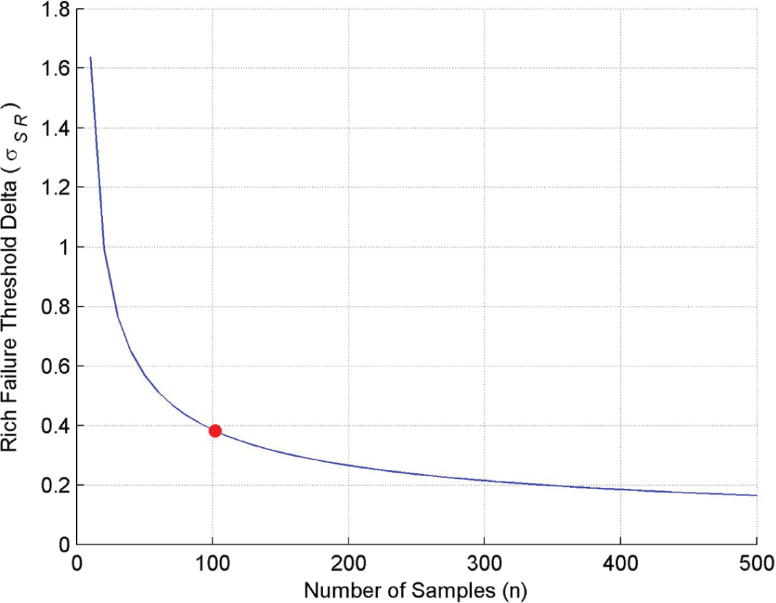
In Figure 4 , the blue solid line shows how the difference between the rich failure threshold and the nominal rich failure threshold, normalised against the value of ${\sigma }_{SR}$ determined at n = 102, decays as the amount of data increases. The red dot shows the current point of rich failure threshold delta. Figure 5 shows the same metric as in Figure 4 but for the lean failure condition.

Figure 4.

Rich failure threshold delta

Figure 5.

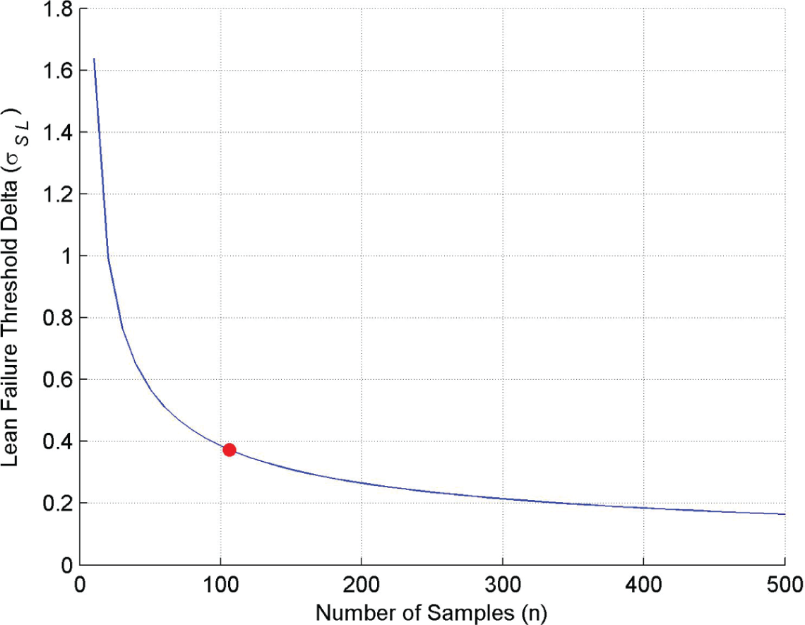
Lean failure threshold delta

From the results shown in Figures 4 and 5, the current set of data obtained at around 100 samples gives an adequate confidence, and subsequent testing would not necessarily lead to a significant change in the values of the failure thresholds. For example, to reduce the current threshold by 50%, in both cases, would require 350 tests to be carried out against the initial data set of 100.

VI. Conclusion

The results in Table 4 show the calculated failure thresholds and the robustness thresholds for rich and lean conditions, and for this diagnostic, there is a significant amount of separation between these two sets of thresholds, enabling the requirements laid out in Section III to be met. This amount of separation has reduced the risk of making use of a Gaussian model to derive the information for the fault-free set of data. If it were the case that there was not such a separation, further investigation would have to be undertaken to understand the reason or to determine perhaps a more valid statistical model.

Table 4.

Summary of the threshold information

	Robust threshold	Failure threshold	Separation
Rich	0.9330	0.8579	$3.46{\sigma }_{L_F}$
Lean	1.0640	1.1647	$4.64{\sigma }_{L_F}$

The use of confidence interval in the statistical models and the threshold setting enables the calibrators to determine when they have collected enough data to provide a robust calibration.