
Abstract
Using a recent result from the program evaluation literature, the author demonstrates that the interpretation of regression estimates of between-group differences in wages and other economic outcomes depends on the relative sizes of subpopulations under study. When the disadvantaged group is small, regression estimates are similar to the average loss for disadvantaged individuals. When this group is a numerical majority, regression estimates are similar to the average gain for advantaged individuals. The author analyzes racial test score gaps using ECLS-K data and racial wage gaps using CPS, NLSY79, and NSW data, and shows that the interpretation of regression estimates varies substantially across data sets. Methodologically, he develops a new version of the Oaxaca–Blinder decomposition, in which the unexplained component recovers a parameter referred to as the average outcome gap. Under additional assumptions, this estimand is equivalent to the average treatment effect. Finally, the author reinterprets the Reimers, Cotton, and Fortin decompositions in the context of the program evaluation literature, with attention to the limitations of these approaches.
Despite five decades of progress since the civil rights movement, black–white gaps in economic outcomes persist in the United States. Much research has focused on racial differences in wages (Neal and Johnson 1996; Lang and Manove 2011), labor force participation (Boustan and Collins 2014), unemployment (Ritter and Taylor 2011), home ownership (Collins and Margo 2001; Charles and Hurst 2002), wealth (Blau and Graham 1990; Barsky, Bound, Charles, and Lupton 2002), cognitive skills (Fryer and Levitt 2004, 2006, 2013; Bond and Lang 2013), non-cognitive skills (Elder and Zhou 2017), infant mortality (Elder, Goddeeris, and Haider 2016), and other outcomes. Recent surveys of this topic—and the related problem of racial discrimination—include Charles and Guryan (2011), Fryer (2011), and Lang and Lehmann (2012). Even after controlling for many observable characteristics of individuals, a typical study finds a significant black–white gap that remains unexplained.
Traditionally, unexplained gaps in mean outcomes have been examined using decomposition methods (see, e.g., Elder, Goddeeris, and Haider 2010; Fortin, Lemieux, and Firpo 2011; Firpo 2017). As noted by Charles and Guryan (2011), however, in recent empirical work researchers have typically focused on a simpler approach of estimating the following model using ordinary least squares (OLS):

where
In this article, I borrow from the recent program evaluation literature to illustrate some important limitations of this approach. As discussed by, among others, Angrist (1998), Humphreys (2009), and Słoczyński (2018), OLS estimation of a model analogous to Equation (1) does not recover, in general, the average treatment effect (ATE), unless the effects of the treatment are homogeneous. These results extend to studies of between-group differences in economic outcomes. In particular, this article demonstrates that the interpretation of regression estimates of such differences depends on the relative sizes of the subpopulations under study (e.g., blacks and whites), which is a straightforward extension of a recent result in Słoczyński (2018). While the previous literature on the interpretation of the OLS estimand has focused on treatment effects, in this article I explicitly consider a framework in which the main variable of interest is an “attribute,” in the sense of Holland (1986), and thus cannot possibly constitute a “treatment” in any actual experiment. Note, however, that this distinction between causal inference and decomposition analysis has implications for how we label our parameters of interest but not for the algebra of least squares, which forms the basis of the results in Angrist (1998), Humphreys (2009), and Słoczyński (2018).
This article concentrates particularly on the following implication of the result in Słoczyński (2018). If we refer to one of the groups as “disadvantaged” (e.g., blacks) and to the other as “advantaged” (e.g., whites), then regression estimates will be similar to the average loss for disadvantaged individuals under the condition that they also constitute a numerical minority. When instead these individuals are a numerical majority—albeit disadvantaged—regression estimates will be similar to the average gain for advantaged individuals.
This relationship between the interpretation of regression estimates and the relative sizes of subpopulations under study is illustrated empirically in several applications to racial gaps in test scores (using data from the Early Childhood Longitudinal Study-Kindergarten [ECLS-K]) and in wages (using data from the Current Population Survey [CPS], the National Longitudinal Survey of Youth [NLSY79], and the National Supported Work [NSW] Demonstration). Compared with the ECLS-K, CPS, and NLSY79 data, in which the proportion of blacks is relatively low, the interpretation of regression estimates is very different in the NSW data, in which blacks constitute a numerical majority. Methodologically, I also develop a new version of the Oaxaca–Blinder decomposition (Oaxaca 1973; Blinder 1973) in which the “unexplained component” could be interpreted as the average treatment effect if we decided to invoke the potential outcome model (see, e.g., Holland 1986; Imbens and Wooldridge 2009). Since it is preferable to treat demographic characteristics as attributes, I usually refer to this object as the average outcome gap—an equivalent parameter that lacks a causal interpretation. Finally, I also provide treatment-effects reinterpretations of the Reimers (1983), Cotton (1988), and Fortin (2008) decompositions. Each of these procedures is easily shown to recover some generally uninteresting convex combination of conditional average outcome gaps.
Theory
Consider a population divided into two mutually exclusive categories, indexed by

namely, the expected value of the conditional average outcome gap over

respectively. Similarly, under certain conditions, these parameters can be regarded as equivalents of the average treatment effect on the treated,

Thus, a particular weighted average of the average gain for advantaged individuals and the average loss for disadvantaged individuals is equal to the average outcome gap.
It should be noted that without further assumptions
This assumption restricts the analysis to counterfactuals that are based on the observed conditional mean for the other group. In other words, the observed conditional mean of advantaged individuals provides a counterfactual for disadvantaged individuals, and vice versa. It should be noted that this assumption rules out the presence of general equilibrium effects, and this might be a substantial restriction in some empirical contexts.
The overlapping support assumption ensures that no combination of observed characteristics can be used to identify group membership. This restriction might be somewhat controversial in the context of black–white differences in economic outcomes, as it is likely that many black or white individuals might have few counterparts in the other subpopulation; clearly, similar problems can also arise in other empirical contexts.
This assumption rules out the presence of unobserved characteristics, which would be correlated with both group membership and outcomes, conditional on observed covariates. For example, this requirement would be violated in the case of black–white differences in wages if school quality were correlated with both wages and race (conditional on
Note that Assumptions 1, 2, and 3 guarantee identification of the aggregate decomposition (Fortin et al. 2011). If we maintain these assumptions, we can construct a counterfactual distribution, which would be observed if the outcomes of disadvantaged individuals were determined according to the conditional mean of advantaged individuals, and vice versa. This counterfactual experiment provides a meaningful interpretation of
Arguably,
Regression Estimates
As noted previously, researchers often analyze between-group differences in economic outcomes by means of OLS estimation of the simple linear model:

Now, unlike in Equation (1), the disadvantaged group is the omitted category.
3
This ensures that the sign of
Słoczyński (2018) studied the interpretation of regression estimates in a model analogous to Equation (5) in which

where
In this article, I focus on a setting in which

where
In other words, if there are many disadvantaged individuals (e.g., blacks), the weight on the average loss for these individuals,

This result has important implications for the interpretation of
Conversely, when we focus on black–white gaps in economic outcomes, the disadvantaged group (i.e., blacks) also constitutes a numerical minority, at least in the United States. In this case,
Of course, blacks do not constitute a numerical minority in all studies of black–white differences in economic outcomes. Sometimes we might intentionally focus on a population that is predominantly black. For example, Stiefel, Schwartz, and Ellen (2006) analyzed test score gaps in a big-city school district. In some countries, such as South Africa, blacks are both disadvantaged and a numerical majority (Sherer 2000; Allanson and Atkins 2005). In either of these cases, regression estimates would be similar to an estimate of the average gain for whites,
Oaxaca–Blinder Decompositions
The simplest solution to this problem with regression estimates is to allow the regression coefficients to be different for both groups of interest:

Also,

where the first element,

The difference between Equations (10) and (11) rests on using alternate comparison coefficients to calculate the explained component as well as measuring the distance between the regression functions,

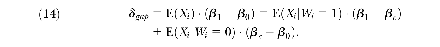
Traditionally, the decomposition literature regards the choice of the comparison coefficients in this context—in other words, the choice between Equations (10) and (11)—as necessarily ambiguous. A number of studies have suggested alternative solutions to this comparison group choice problem. Such an approach is often referred to as “generalized” Oaxaca–Blinder, and it involves an alternative decomposition:
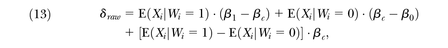
where
As noted previously, several papers have suggested alternative comparison coefficients for Equation (13). These coefficients are often of the form
Recovering the Average Outcome Gap
A number of studies (Barsky et al. 2002; Black, Haviland, Sanders, and Taylor 2006, 2008; Melly 2006; Fortin et al. 2011; Kline 2011) have noted that the unexplained component in Equation (10) can be interpreted as
In fact, this result follows from the choice of

A proof of Proposition 1 follows immediately from simple algebra. Perhaps surprisingly, the choice of
Interestingly, this alternative decomposition is equivalent to a flexible linear regression model for the average treatment effect, discussed in Imbens and Wooldridge (2009) and Wooldridge (2010). If
which is equivalent to the decomposition in Proposition 1. Similarly, the unexplained component of the decomposition in Equation (10) is equal to the coefficient on
Several recent articles have criticized the dependence of traditional decomposition methods on linear conditional means (Barsky et al. 2002; Frölich 2007; Ñopo 2008). Thus, it is useful to clarify that the main insight underlying Proposition 1 is unrelated to the linearity assumptions in Equation (9). If we write the counterfactual conditional mean as
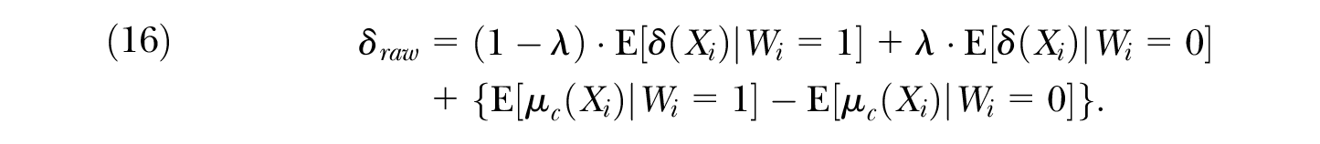
As before, the choice of
Estimation of
Interpreting the Explained Component
Traditionally, decomposition methods have been used to provide estimates of both the unexplained and explained components. The interpretation of the explained components in Equations (10) and (11) is well known. Similarly, it might be useful to clarify the interpretation of the explained component in Proposition 1,
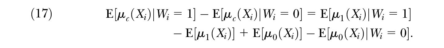
We can easily interpret both elements of this explained component. The first element,
Of course, the same interpretation holds in the case of the explained component in Proposition 1,
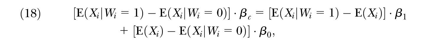
which is a linear special case of Equation (17). Fortin et al. (2011) also briefly discussed a similar explained component.
Reinterpreting Reimers (1983), Cotton (1988), and Fortin (2008)
Finally, the logic of Proposition 1 applies also to several versions of the Oaxaca–Blinder decomposition in Reimers (1983), Cotton (1988), and Fortin (2008). We can easily verify that 1) the unexplained component of the Reimers (1983) decomposition is equal to the arithmetic mean of
To be clear, these interpretations of the Reimers (1983), Cotton (1988), and Fortin (2008) decompositions assume simple counterfactual treatment (Assumption 1), whereas this assumption is not invoked in any of these studies. More precisely, each tries to account for the presence of general equilibrium effects, which are ruled out by Assumption 1, and to derive a counterfactual conditional mean, which would be observed—in the context of wage gaps—if discrimination ceased to exist. It is very difficult, however, to correctly guess the form of this “nondiscriminatory” or “competitive” wage structure—and Reimers (1983), Cotton (1988), and Fortin (2008) did not offer any theoretical basis to rationalize their choices. Here it might be easier to invoke the assumption of simple counterfactual treatment instead of relying on the general equilibrium approach. In this case, the Reimers (1983), Cotton (1988), and Fortin (2008) decompositions would be problematic.
Black–White Differences in Test Scores and Wages
Clearly, the interpretation of regression estimates of black–white gaps in economic outcomes depends on the relative sizes of black and white subsamples. Still, OLS estimation of the model in Equation (5) constitutes a standard approach in empirical work (Charles and Guryan 2011). While we can always solve this problem using a variety of semi- and nonparametric methods, it might be sufficient to use one of several versions of the Oaxaca–Blinder decomposition. To estimate
These methodological considerations will be illustrated in various empirical applications to black–white differences in test scores and wages. Whenever blacks are a numerical minority, regression estimates will be similar to their average loss. When, however, blacks become a disadvantaged majority, regression estimates will mimic the average gain for whites. Yet, the estimates based on decomposition methods will always have the desired interpretation:
Black–White Test Score Gaps in ECLS-K
Following Neal and Johnson (1996), labor economists widely agree that a substantial portion of the black–white wage gap is a consequence of differences in premarket factors. Consequently, in an attempt to explain the emergence of this gap, many researchers have focused on education and cognitive development in children. An example is Fryer and Levitt’s (2004) influential study of the black–white test score gap in kindergarten and first grade. This research concluded that the gap among incoming kindergartners practically disappeared when controlling for a small number of covariates. It appeared, however, to re-emerge during the first two years of school.
Recent follow-up studies by Bond and Lang (2013) and Penney (2017) have focused on the (lack of) robustness of these conclusions related to the ordinality of test scores. More precisely, Fryer and Levitt (2004) have treated test scores as interval scales, even though this is inappropriate and any monotonic transformation of the test score scale is also a valid scale. On the one hand, using several such transformations, Bond and Lang (2013) have cast doubt on many of the conclusions in Fryer and Levitt (2004). On the other hand, Penney (2017) considered a normalization of test scores that is invariant to monotonic transformations; his preferred estimates were very similar to regression estimates in Fryer and Levitt (2004). In this article, I ignore the issue of ordinality of test scores and focus on the interpretation of regression estimates of the black–white test score gap as a weighted average of the average gain for whites and the average loss for blacks. In this sense, my analysis should be treated as an illustration of a different methodological issue, rather than a stand-alone contribution to the debate on black–white test score gaps.
All of these previous papers—namely, Fryer and Levitt (2004), Bond and Lang (2013), and Penney (2017)—are based on data from the ECLS-K. The sample included more than 20,000 children who entered kindergarten in 1998. The main outcomes of interest are standardized test scores in math and reading. I borrow the sample and covariate selections from Penney (2017), who followed Fryer and Levitt (2004). However, unlike Penney (2017), I restrict my attention to test scores in the fall and spring of kindergarten and drop individuals whose race is coded as Hispanic, Asian, or other.
Table 1 reports regression estimates of the black–white test score gap and supplements them with estimates of
Black–White Test Score Gaps in ECLS-K
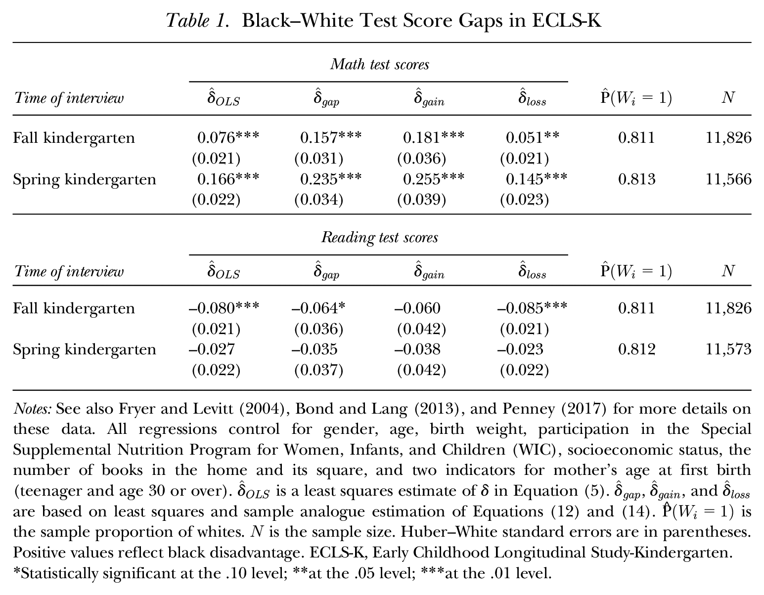
Notes: See also Fryer and Levitt (2004), Bond and Lang (2013), and Penney (2017) for more details on these data. All regressions control for gender, age, birth weight, participation in the Special Supplemental Nutrition Program for Women, Infants, and Children (WIC), socioeconomic status, the number of books in the home and its square, and two indicators for mother’s age at first birth (teenager and age 30 or over).
Statistically significant at the .10 level; **at the .05 level; ***at the .01 level.
At the same time, the minority status of blacks has an additional consequence. Namely, the estimated average gaps and average gains for whites are always very similar. In the case of math test scores, they are also quite different from both
To be clear, it is not unreasonable to believe that
Black–White Wage Gaps in CPS
Many studies have documented that the trend toward black–white wage convergence stopped in the mid-1970s or around 1980 (see, e.g., Grogger 1996; Chay and Lee 2000; Juhn 2003; Bayer and Charles 2018). While some research has also revealed a sharp decline in the black–white wage gap in the 1990s (Juhn 2003), other studies have not (Elder et al. 2010). Moreover, several recent contributions have concluded that the current magnitude of the racial wage gap in the United States is the largest in several decades (see, e.g., Hirsch and Winters 2014; Bayer and Charles 2018).
In this article, as in Juhn (2003) and Elder et al. (2010), I focus on data from the March CPS, which are distributed by Flood, King, Ruggles, and Warren (2017). I also borrow the sample and covariate selections from Elder et al. (2010) and extend their analysis by 10 years, from 2008 to 2017. Thus, I study a subsample of full-time, full-year working males; this category is defined as those participants who are at least 18 years old, have earned non-zero wage or salary income, and have worked more than 40 weeks a year and 30 hours in a typical week. Following Elder et al. (2010), I also restrict my attention to individuals whose race is coded as either black or white. The outcome variable of interest is the log hourly wage, and the hourly wage is measured as annual earnings divided by annual hours. The set of control variables is relatively sparse and is listed in Table 2.
Black–White Wage Gaps in the Current Population Survey (CPS)
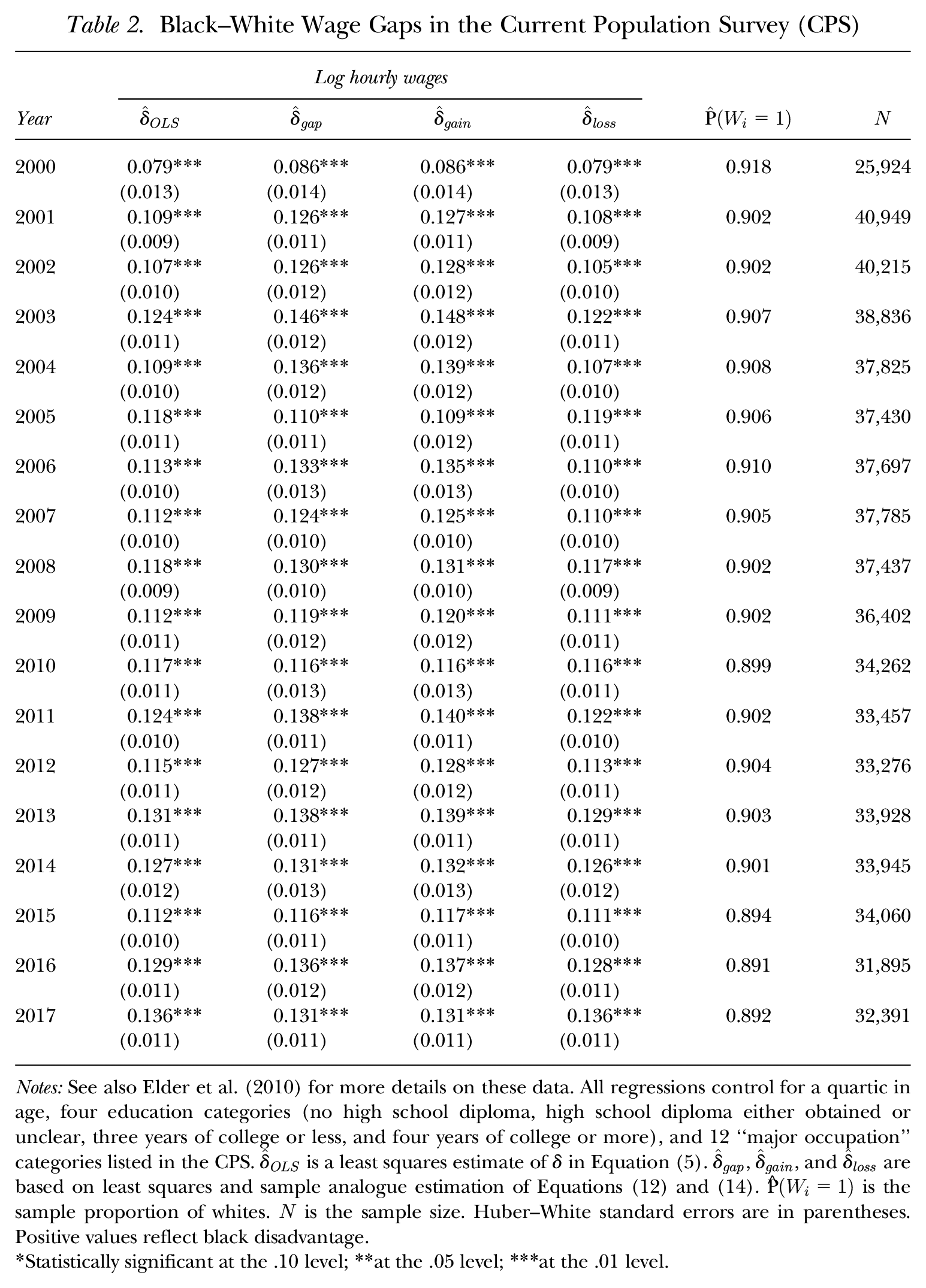
Notes: See also Elder et al. (2010) for more details on these data. All regressions control for a quartic in age, four education categories (no high school diploma, high school diploma either obtained or unclear, three years of college or less, and four years of college or more), and 12 “major occupation” categories listed in the CPS.
Statistically significant at the .10 level; **at the .05 level; ***at the .01 level.
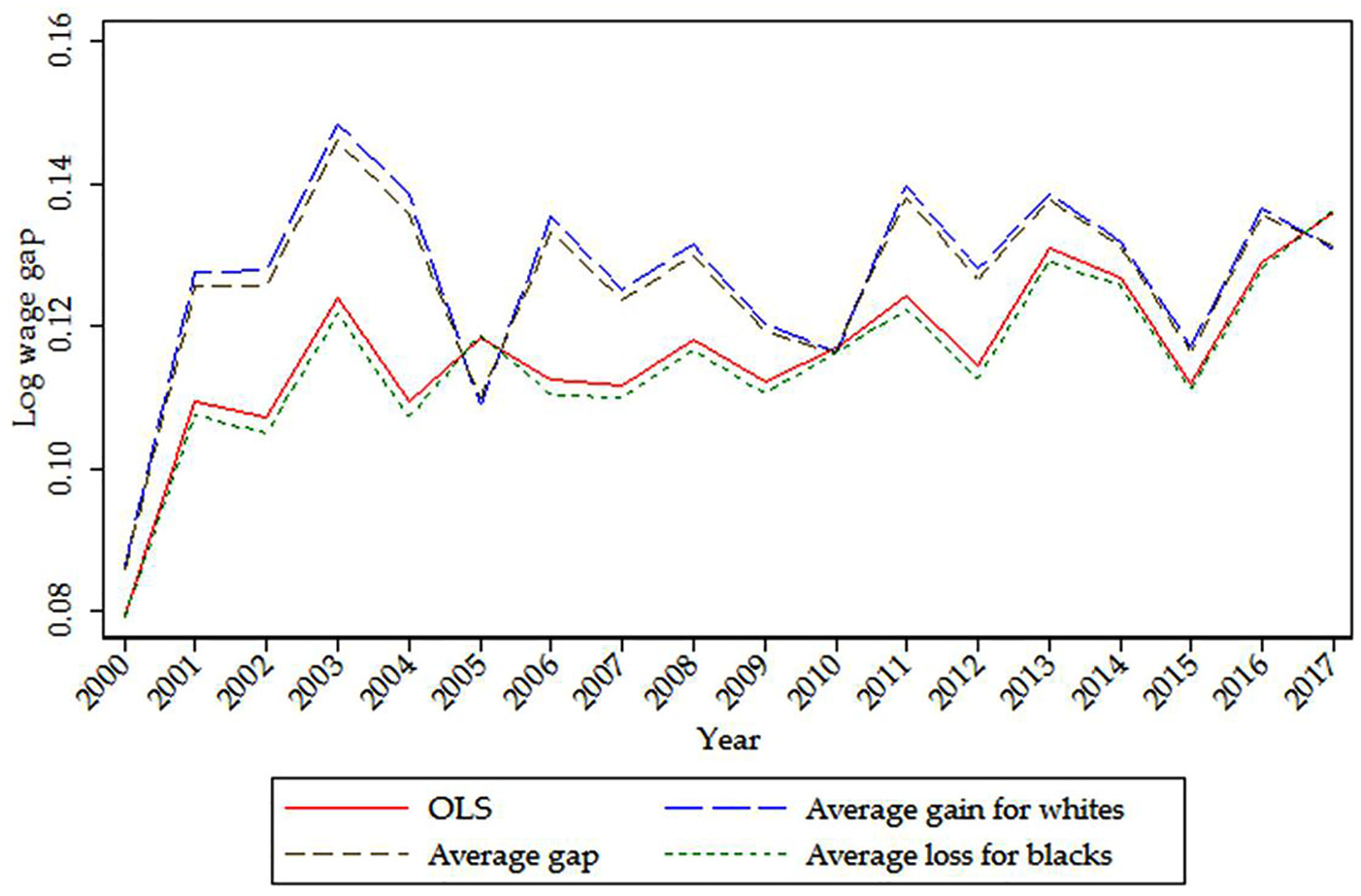
Table 2 and Figure 1 report the estimates of
Black–White Wage Gaps in the Current Population Survey (CPS)
It should also be noted that, generally speaking, the differences between the average loss for blacks and the average gain for whites are rather small in the CPS data, and hence
Black–White Wage Gaps in NLSY79
A common concern about the CPS data is that it lacks information about some important determinants of wages. In particular, Neal and Johnson (1996) demonstrated that the black–white wage gap nearly disappeared after controlling for age and performance on the Armed Forces Qualifying Test (AFQT). Unsurprisingly, this measure of ability is unavailable in most microeconomic data sets, including CPS. It is recorded, however, as part of the NLSY79, which is a panel study of individuals born between 1957 and 1964 that began in 1979 and which was also the source of data in Neal and Johnson (1996).
More recently, Lang and Manove (2011) built a model of educational attainment predicting that, conditional on ability (as proxied by AFQT scores), blacks should receive more education than whites. On the basis of this model, whose predictions are broadly consistent with the NLSY79 data, Lang and Manove (2011) recommended that one should control for both AFQT scores and education when studying black–white differences in wages. Interestingly, when Lang and Manove (2011) augmented the specifications of Neal and Johnson (1996) with education, a substantial black–white wage gap re-emerged.
In this article, I borrow the sample and covariate selections from Lang and Manove (2011: table 5). Because I focus entirely on the black–white gap, I also drop all Hispanics. I study log hourly wages of black and white men from the 1996, 1998, and 2000 waves of the survey. The list of control variables is reported in Table 3, together with regression estimates of the black–white wage gap as well as estimates of
Black–White Wage Gaps in NLSY79
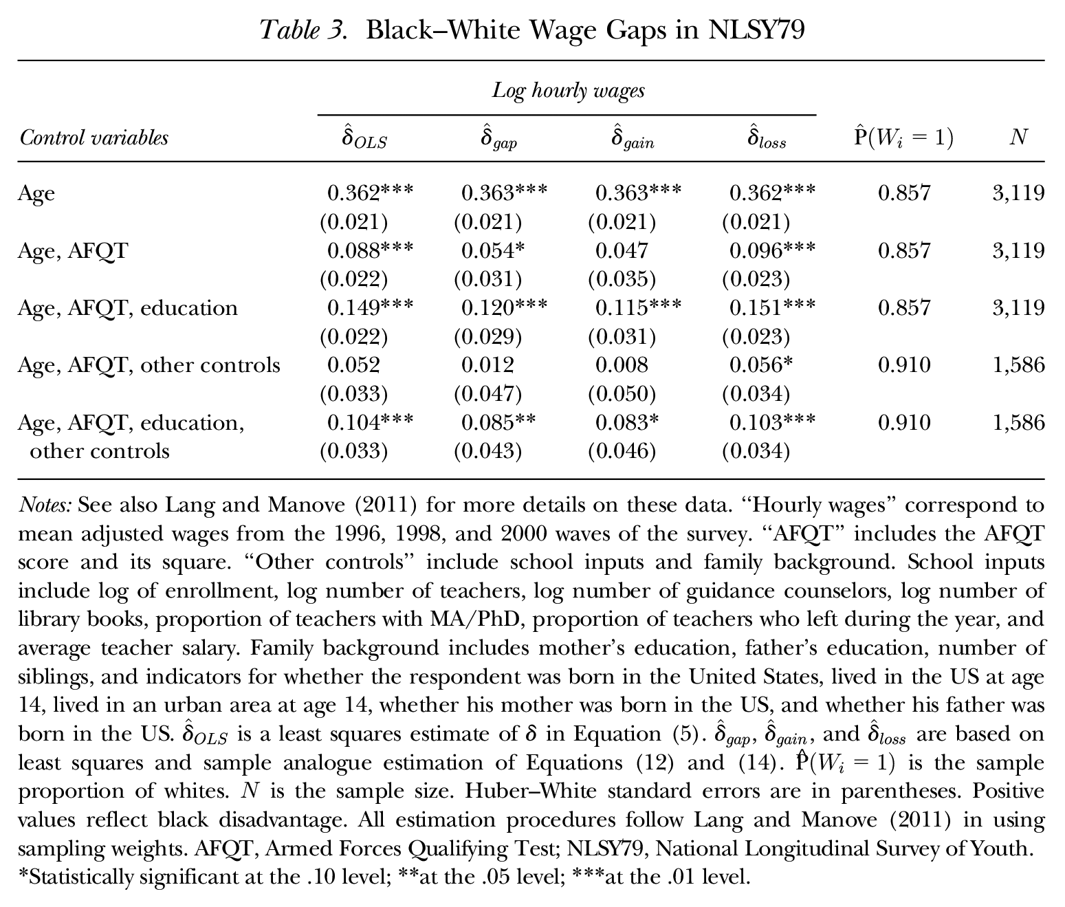
Notes: See also Lang and Manove (2011) for more details on these data. “Hourly wages” correspond to mean adjusted wages from the 1996, 1998, and 2000 waves of the survey. “AFQT” includes the AFQT score and its square. “Other controls” include school inputs and family background. School inputs include log of enrollment, log number of teachers, log number of guidance counselors, log number of library books, proportion of teachers with MA/PhD, proportion of teachers who left during the year, and average teacher salary. Family background includes mother’s education, father’s education, number of siblings, and indicators for whether the respondent was born in the United States, lived in the US at age 14, lived in an urban area at age 14, whether his mother was born in the US, and whether his father was born in the US.
Statistically significant at the .10 level; **at the .05 level; ***at the .01 level.
The second and fourth rows of Table 3 correspond to the specifications of Neal and Johnson (1996). It turns out that focusing on the average wage gap, as opposed to regression estimates, would have strengthened their conclusions. Even though
At the same time, the main conclusion of Lang and Manove (2011) still holds true. When we also control for education, as in the third and fifth rows of Table 3, all measures of the black–white wage gap become substantially larger. Still,
Black–White Wage Gaps in NSW
My results on black–white differences in ECLS-K, CPS, and NLSY79 data share an essential feature: in each case,
Following LaLonde (1986), Dehejia and Wahba (1999), and Smith and Todd (2005), many studies have used the data on men from the NSW Demonstration, together with non-experimental data sets constructed by LaLonde (1986), to compare the effectiveness of various identification strategies and estimation methods for average treatment effects. In short, NSW was a US work experience program that operated in the mid-1970s and that randomized treatment assignment among eligible participants. This program served a highly disadvantaged population whose members were disproportionately black (Smith and Todd 2005).
As noted previously, these data are typically used to study the effects of the NSW program itself. There is little reason, however, why they should not be used to study black–white wage gaps, although of course the results may not reflect the magnitudes of these gaps in the whole US population. I analyze the original data on the experimental treatment and control groups, as in LaLonde (1986). To be consistent with the previous empirical applications, I focus on log wages and exclude Hispanics; these two restrictions reduce the sample size to 460 individuals, 87% of whom are black.
Table 4 reports the estimates of
Black–White Wage Gaps in the National Supported Work (NSW) Demonstration
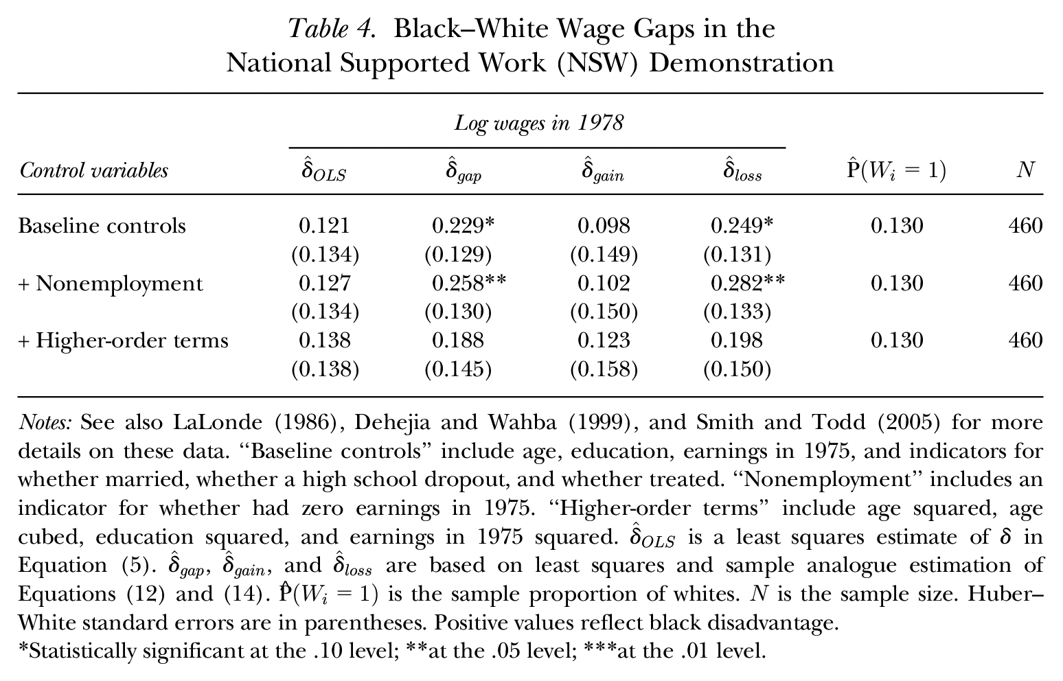
Notes: See also LaLonde (1986), Dehejia and Wahba (1999), and Smith and Todd (2005) for more details on these data. “Baseline controls” include age, education, earnings in 1975, and indicators for whether married, whether a high school dropout, and whether treated. “Nonemployment” includes an indicator for whether had zero earnings in 1975. “Higher-order terms” include age squared, age cubed, education squared, and earnings in 1975 squared.
Statistically significant at the .10 level; **at the .05 level; ***at the .01 level.
Unlike previously, the average loss for blacks is not approximated by
Conclusion
In this article, I have borrowed a recent result from the program evaluation literature to demonstrate that the interpretation of regression estimates of between-group differences in economic outcomes necessarily depends on the relative proportions of these groups. If the disadvantaged group is also a numerical minority, as is often the case with blacks, regression estimates will be similar to the average loss for this group. I have demonstrated the empirical relevance of this prediction in applications to black–white test score gaps in ECLS-K data and black–white wage gaps in CPS and NLSY79 data.
Sometimes, however, the disadvantaged group does not constitute a numerical minority, in which case regression estimates will not approximate the average loss for this group. When the majority group is, in fact, disadvantaged—say, blacks in an urban school district, in South Africa, or in NSW data—regression estimates will be similar to the average gain for advantaged individuals. Unfortunately, in most applications, this parameter is also less likely to be of direct interest.
In an intermediate case, where the proportions of both groups are similar—which is to be expected, for example, in a typical study of gender wage gaps—regression estimates will be similar to the average outcome gap. There are reasons to believe that this is an interesting parameter, as it is equal to the difference between mean outcomes in two counterfactual distributions. In the first distribution, outcomes of both groups are determined according to the conditional mean of advantaged individuals. In the second distribution, all outcomes are determined using the conditional mean of disadvantaged individuals.
Of course, instead of relying on regression estimates, researchers may prefer to explicitly choose their parameter of interest. While its estimation would be easy to implement semi- or nonparametrically, following a more traditional approach of using parametric decomposition methods is also possible. If we wish to estimate the average gain for advantaged individuals or the average loss for disadvantaged individuals, we need to use one of the most basic versions of the Oaxaca–Blinder decomposition (Oaxaca 1973; Blinder 1973). If instead we are interested in the average outcome gap, we need to apply the main contribution of this article: a new decomposition whose unexplained component is equal to this parameter. Interestingly, under a particular conditional independence assumption, this object is also equivalent to the average treatment effect.
These decompositions and the framework of this article can be relevant for public policy. For example, Blau and Kahn (2017: 800) explained, without using this particular notation, that
There are also other contexts in which focusing on
What follows, even if we were potentially interested in such general equilibrium effects, focusing instead on
Finally, important empirical contexts exist, in which the notion of a “nondiscriminatory” or “competitive” conditional mean generally does not apply. Among these are black–white gaps in test scores, infant mortality, as well as comparisons of wage structures across time. In these cases, a partial equilibrium approach is perhaps natural, as is the focus on parameters such as
Future work might add to our understanding of formal conditions under which causal effects of race, gender, and other immutable characteristics can be identified and estimated (see Kunze 2008, Greiner and Rubin 2011, and Huber 2015 for recent discussions). As already suggested by Fortin et al. (2011), the economic structure behind decomposition methods should also be improved. Finally, understanding the links between the decomposition methods and the program evaluation literature is essential. Following an important review in Fortin et al. (2011), this article has attempted to take this ongoing discussion one step further by providing an interpretation of regression estimates of between-group differences in economic outcomes and developing a new decomposition compatible with the treatment effects framework.
Footnotes
Acknowledgements
I am grateful to Arun Advani, Joshua Angrist, Anna Baranowska-Rataj, Elizabeth Brainerd, Brantly Callaway, Thomas Crossley, Todd Elder, Steven Haider, Krzysztof Karbownik, Patrick Kline, Michał Myck, Mateusz Myśliwski, Ronald Oaxaca, Pedro Sant’Anna, Jörg Schwiebert, Gary Solon, Adam Szulc, Joanna Tyrowicz, Glen Waddell, Rudolf Winter-Ebmer, Jeffrey Wooldridge, seminar participants at Bank of Canada, Brandeis, CEPS/INSTEAD, and SGH, and participants at many conferences for helpful comments and discussions.
I acknowledge financial support from the National Science Centre (grant DEC-2012/05/N/HS4/00395), the Foundation for Polish Science (a “Start” scholarship), the “Weź stypendium – dla rozwoju” scholarship program, and the Theodore and Jane Norman Fund.
This article builds on ideas from and supersedes my papers, “Population Average Gender Effects” and “Average Wage Gaps and Oaxaca–Blinder Decompositions.” Data and copies of the computer programs used to generate the results presented in the article are available from the author at
1
2
3
In this case, of course, all elements of ![]() .
.
4
Also, for a generic random variable
5
The exact expressions for
6
See, for example, Blau and Beller (1988), Weinberger and Kuhn (2010), and ![]() . Note, however, that none of these three studies restricts its attention to such simple regression estimates.
. Note, however, that none of these three studies restricts its attention to such simple regression estimates.
7
Note that Duncan and Leigh (1985) used a similar decomposition in an application to union wage premiums. ![]() , however, criticized this approach as being “not a very intuitive procedure.”
, however, criticized this approach as being “not a very intuitive procedure.”
9
At first, this finding might seem inconsistent with the stylized fact reported in ![]() that black–white wage gaps decrease with education, to the extent that no significant wage differences occur between high-skilled blacks and high-skilled whites. If this is true, then we should expect
that black–white wage gaps decrease with education, to the extent that no significant wage differences occur between high-skilled blacks and high-skilled whites. If this is true, then we should expect
10
In an earlier working paper version of this article, I focused on the subset of the experimental treatment and control groups constructed by ![]() ; I also did not exclude Hispanics from the sample. Many of the estimates were quite different than currently reported, although the main message remains unchanged: With a large proportion of blacks,
; I also did not exclude Hispanics from the sample. Many of the estimates were quite different than currently reported, although the main message remains unchanged: With a large proportion of blacks,