
Abstract
The stock market is the reflection of the trading pattern of various investors. The present study attempts to examine the trading behaviour followed by foreign institutional investors, domestic institutional investors and mutual funds during 2010–2020 in the Indian stock market. The whole time period is divided into two subperiods using the chow breakpoint test. Two vector autoregression framework models accompanied with impulse response function and variance decomposition analysis are employed in both the subperiods, namely calm period and volatile period. It is found that the institutional investors do not pay heed to the market returns in the calm period, while the interdependency among the institutional investors increases in the volatile period. The structural break enhances the forecasting accuracy of the model significantly. This study will help the government to understand the impact of calm period and volatile period on the trading behaviours of the institutional investors and thereby their sentiments in the Indian stock market.
Keywords
Introduction
The stock market of any country is claimed to be a function of the trading behaviour manifested by the institutional investors. There are broadly three important types of institutional investors which are believed to paint the stock markets with the colour of their trading patterns. Foreign institutional investors (FIIs), domestic institutional investors (DIIs) and mutual funds (MFs) are the investors which hold great power and either get influenced by the market returns or influence the market return. The momentum of trading for all the three types of investors has increased enormously.
Indian market is looked at as a profitable investment destination by institutional investors. To ratify this fact, India stood at the sixth position in the world with respect to nominal GDP and at the third position with respect to purchasing power parity at the end of 2020. Moreover, India was the second capable country after China in converting the net withdrawal of funds in March 2020 due to the nationwide lockdown to net infusion of funds in June 2020 among the BRICS countries. In other words, investors perceive Indian market as a promising destination despite it being a developing nation. Thus, Indian market brings a sense of curiosity and, therefore, must be studied in context with the behaviour exhibited by the investors during trading in the Indian market. The Indian market has seen an extreme condition in its macroeconomic variables during the lost decade (2010–2020), and thus, the authors believe that the trading patterns of the investors must have altered simultaneously (Kumar et al., 2021; Sibande et al., 2021; Vardhan & Sinha, 2016). To corroborate, the Indian GDP was in double digits in the first quarter of 2010 but dwindled down and reached in negative territory at the end of the decade; thus, the term ‘lost decade’ has been coined for this period. Thus, the selected time frame, division of the time span – calm period and volatile period and, lastly, the trading behaviour of the institutional investors is a judicious mix of understanding the Indian stock market.
To emphasise, the trading behaviour of the investors dictates the movement of the stock market index due to the large involvement depicted by them, both in isolation and in herding patterns as found by previous research studies (Chittedi, 2014; Kim & Wei, 2002). A majority of the studies in the past have focused upon understanding the trading behaviour depicted by FIIs and DIIs. MFs are often ignored to be studied separately as it is a category within the DIIs. Further, a comparative analysis of the trading patterns of all the three institutional investors, that is, FIIs, DIIs and MFs, remains as a research gap which is yet to be studied. It is important to consider MFs as they have grown tremendously from J25 crore assets under management in 1965 to J31.64 lakh crore in 2021.
Therefore, the objective of the current study is to analyse the trading behaviour of the three institutional investors, namely FIIs, DIIs and MFs during 2010–2020. The selected time frame has been divided into two sample periods based upon the structural break found using the chow breakpoint test. Our results suggest that the trading behaviour of the institutional investors remains the same in both the subperiods, but the magnitude and their relation among themselves change significantly. The results of the current study contribute to the existing literature in a significant manner and refute the findings of Boot and Pick (2020).
Review of Literature
An extensive literature review has been conducted based on the Indian and international studies. Some of the studies in the Indian and international contexts are as follows:
Indian Studies
A long-lasting debate exists in deciding the role played by the FIIs in the Indian scenario. Some research works claim foreign investors to have an upper hand when compared to the DIIs in influencing the stock market returns. In other words, foreign investors have a higher influential power than the domestic investors (Pal, 1998). FIIs are largely associated to have a positive correlation with the Indian stock market (Mishra et al., 2009; Sehgal & Tripathi, 2009). In other words, the majority of the past research concludes that foreign investors follow a positive feedback trading strategy (Bhanumurthy & Singh, 2013; Bose, 2012; Mehla & Goyal, 2013). One startling fact to take into consideration is that Pal (1998) and Ananthanarayan et al. (2009) claim that foreign investors do not impact the stock markets significantly, while Mehla and Goyal (2013) claim that foreign investors influence the Indian stock market significantly. Mishra (2015) found that foreign investors and domestic investors follow opposite trading strategies. In other words, when the market return surges, the foreign investors buy and domestic investors sell (Arora, 2016; Bansal & Rao, 2018; Chauhan & Chaklader, 2020; De & Ghosh, 2019; Jalota, 2017; Raphael & Jacob, 2018; Sathish, 2020). It can also be deduced that foreign investors are return chasers. Lastly, it is also reported by the past studies that domestic investors feed upon the discarded stocks of foreign investors (Bhanumurthy & Singh, 2013; Jalota, 2017). To its contrary, Badhani and Kumar (2020) reports that FIIs and DIIs do not have superior market timing skills.
However, all the studies do not provide a comparative analysis of the trading behaviour depicted by the three major institutional investors in the Indian stock market.
International Studies
A brief literature review has also been conducted with respect to international countries or international groups. It is important to take into consideration the trading strategies adopted by the institutional investors worldwide. Therefore, an attempt has been made to cover international studies so as to build up a generalised view about the trading behaviour exhibited by the institutional investors.
The trading behaviour adopted by the foreign institutional investors is widely reported in the past research work. Research work by Stulz (1999) concludes that foreign investors do not actively contribute towards the upliftment of capital markets post-liberalisation, while Froot et al. (2001) claim that foreign investors have the ability to predict the future returns, especially in the emerging nations. Kim and Wei (2002) have reported the trading behaviours in the context of FIIs and foreign individual investors. It is found that FIIs follow a positive feedback trading strategy, while the individual investors follow a negative feedback trading strategy. The same is reported by Cai and Zheng (2004) and Boyer and Zheng (2009). Kim and Yi (2015) have reported that DIIs invest with a long-term perspective. Schuppli and Bohl (2010) found that DIIs follow a positive feedback trading strategy in the B-share markets post-liberalisation and FIIs do not destabilise the Chinese A-share markets. Zou et al. (2016) also report the opposite trading strategies adopted by FIIS and DIIs.
Therefore, it can be seen that MFs are less studied despite their tremendous growth in the Indian scenario. Thus, we made an attempt to cover all the three major institutional segments to examine the trading behaviour followed by each one of them during the lost decade.
Hypotheses in the Study
According to the review of literature and the objective, following are the hypotheses:
Research Methodology
Data and Sample
The present study conducted a comparative analysis of the trading behaviour depicted by the FIIs, DIIs and MFs in the Indian stock market during 2010–2020. The selected time frame can be recalled as a lost decade for the Indian economy on account of GDP growth. The GDP growth was as high as 11.4% in the first quarter of 2010 but headed its journey towards a downward slide from 2018 onwards. Moreover, COVID-19 exacerbated the GDP growth in the negative territory in 2020. Also, the selected time frame is important to study because of the political events which happened and affected the trading pattern of the investors. The political events like the Shanghai crash in 2015 witnessed a surge in foreign flows in the Indian stock market; demonetisation in 2016, the goods and services tax regime in 2017 and, lastly, the COVID-19 pandemic in 2020 make this period an important period to study. It is vital to study the behaviour of institutional investors during such an unstable period. The methodology adopted in the present study has been employed in prior research works too, thus confirming the right selection of tools and techniques (Bansal & Rao, 2018; Froot et al., 2001; Naik & Padhi, 2015; Vardhan & Sinha, 2016).
Variables Used in the Study
The trading pattern of the investors can be best captured by their net flows in totality. In other words, net flows of institutional investors include the purchasing and selling activities, and thus, it is the most suitable variable for measuring the trading activity exhibited by the investors. The variables selected in the present study are net flows arising from foreign institutional investors (FIIN), domestic institutional investors (DIIN) and mutual fund (MFN). The daily frequency of the net flows has been considered during the selected time frame for gauging the behaviour. Nifty 50 return proxies the Indian market return because it covers a diversified portfolio of 50 stocks. Therefore, Nifty 50 returns are used as the benchmark index in the current study (NSER).
Tools and Techniques
To discern the trading behaviour exhibited by the institutional investors in the Indian scenario, we applied the vector autoregression framework (VAR) accompanied with the impulse response function (IRF) and variance decomposition analysis (VDA) using Eviews 11 version. The VAR framework considers all the variables as endogenous, and it gauges each variable by the lag values of other variables and its own lag value. It is best suited for the multivariate time series and for the present study in discerning the trading behaviour of the institutional investors in the Indian scenario. It can be best understood through Equation (1).

Where
yt = The k endogenous variables are collected in the yt vector.
t = Each period of time is numbered 1, …, t.
yt − p = It denotes that the value of the variable is p periods earlier than the current period. In other words, it represents the lag value of that variable.
Ai = Time invariant matrix.
et = k-vector of error terms.
To apply the VAR framework for analysing the interrelationship among the endogenous variables, it is necessary to determine the stationarity of the variables. For checking the presence of the unit root and thereby stationarity or non-stationarity, the augmented dickey fuller (ADF) test has been used. The presence of unit root indicates non-stationarity in the time series, which leads to spurious regression results. The basic form of the ADF equation is given in Equation (2):

Where
Yt is the time series at t time period;
Xe is the set of exogeneous variable; and
α is the coefficient of the first lag on Y
Further, to determine the optimum number of lags in the model, the Schwarz information criterion (SIC) is used. SIC has a better forecasting accuracy and leads to the selection of efficient order models (Koehler & Murphree, 1988; Poskitt, 1994; Shittu & Asemota, 2009).
Further, the established models were checked for parameter stability and misspecification in the model using the cumulative sum control chart (CUSUM) and Ramsey regression equation specification error test (RESET). Also, to check the serial correlation, the Breusch–Godfrey serial correlation LM test was used. Further, in order to find the behaviour of institutional investors during different periods, structural break was found using the chow breakpoint test.
It is important to identify trading behaviour in favourable and unfavourable situations persisting in an economy. It is believed by some researchers that recognising the structural break in the sample period leads to improved accuracy (Pettenuzzo & Timmermann, 2011), while other researchers claim that identifying structural break does not significantly increase the forecasting and accuracy of the model (Boot & Pick, 2020; Stock & Watson, 1996). Therefore, in order to verify the significance of structural break, we checked for the structural breaks using the Chow breakpoint test. The significant breakpoint was found on 13 April 2020. A study by Boot and Pick (2020) claims that any structural break occurring in the later part of the sample does not improve the accuracy of the model significantly. However, we chose to include the structural break to examine the difference in the results of the two subperiods, if any, as opposed to the findings of Boot and Pick (2020). As a result, we divided our selected time frame into two periods ranging from 1 January 2010 to 12 April 2020 and 13 April 2020 to 31 December 2020. The output for the significance of the breakpoint is given in Table 1.
Chow Breakpoint in the Sample Period.
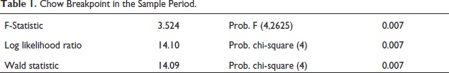
Chow Breakpoint in the Sample Period.
We termed the first period ranging from 1 January 2010 to 12 April 2020 as the calm period because the stock market did not experience any havoc during this period despite the falling GDP while the second period ranging from 13 April 2020 to 31 December 2020 as the volatile period due to the stock market crash due to COVID-19. The structural break was created due to COVID-19, leading to Indian stock market crash. The analysis of the VAR framework, IRF and VDA has been conducted for both the periods to diagnose the behaviour of institutional investors in the calm and volatile periods.
VAR Framework
Table 2 produces the results regarding the stationarity of the variables used in both the models.
Stationarity of Selected Variables (Net Investments).
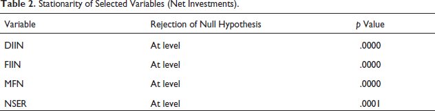
All the variables are stationary at 1% level of significance. Thus, the selected variables can be used in the VAR framework for analysis purpose in different time frames.
The equations tested for in the VAR framework are as follows:


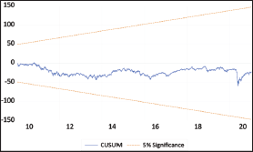
In all the equations, each endogenous variable is explained by its own lag value and lagged value of other variables. Before applying the VAR framework, the model was checked for stability using CUSUM test.
Figure 1 indicates that the blue line denoting cumulative sum based on recursive residuals does not go outside the critical lines, and hence, we can say that there is a stability in parameters. Also, RESET test was conducted for checking any misspecification present in the model. The results suggest that RESET statistic is 2.06 with p value = .1534, which is more than .05, which indicates that there are no misspecifications present in the model.
CUSUM Test at 5% Level of Significance for VAR Model.
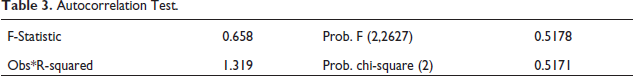
Further, we have also checked for any serial autocorrelation present in the residuals using the Durbin Watson test and Breusch–Godfrey serial correlation LM test. The results indicate that there is no autocorrelation present in the model. The results of the Breusch-Godfrey serial correlation LM test can be seen in Table 3. It indicates that the null hypothesis claiming no serial correlation has been accepted as the p value is greater than .05. Also, the Durbin Watson test shows a value of 1.987, and therefore, it is safe to believe that our model does not have the problem of autocorrelation.
Autocorrelation Test.
VAR Results for the Calm Period
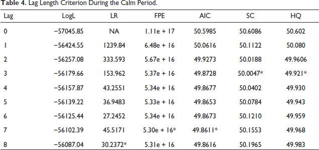
The lag value used in the model is selected as 3 according to the Schwarz information criterion as shown in Table 4.
Lag Length Criterion During the Calm Period.
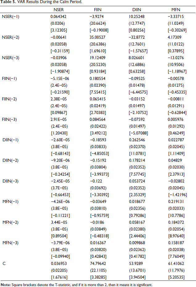
The VAR results depicting the trading behaviour of the institutional investors during the calm period are given in Table 5. The result depicts that market return does not influence FIIN and MFN. Moreover, it can be observed that FIIN and DIIN move opposite to each other, while MFN and DIIN move in the same direction.
VAR Results During the Calm Period.
We employ IRF to better understand the trading pattern of the investors. Figure 2 shows the result obtained by employing IRF.
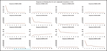
The figure clearly depicts that FIIs and DIIs follow a trading strategy opposite to each other. It can be noticed that none of the investors respond aggressively to changes in the market return, but it is clearly observable that FIIs respond positively to NSER while DIIs respond negatively to NSER. However, mutual funds do not respond significantly to the market returns proxied by NSER but respond contrary to the trading patterns followed by FIIs. Thus, we can conclude that neither the MFs respond to the changes in any of the other endogenous variables present in the model actively nor do they influence other variables. Thus, MFs act as passive investors during the calm period. A similar result has been obtained by Bhanumurthy and Singh (2013).
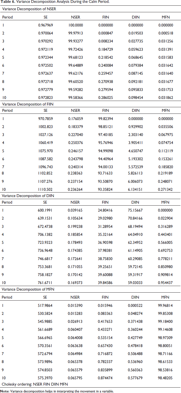
Further, we employed VDA to find out the cause of the variance in each of the endogenous variable. Table 6 shows the result for VDA. The results signify that DIIs are highly influenced by the trading pattern adopted by the foreign investors. The variance in the MFs is caused by itself and not by other variables present in the model. In other words, MFs are not interdependent on any of the other variables and invest on the information possessed by themselves. It is also observed that domestic investors are highly efficient in influencing the market returns than foreign investors (Kotishwar & Alekhya, 2015).
Variance Decomposition Analysis During the Calm Period.
Thus, it can be concluded that when the economic position is calm and favourable in terms of GDP growth rate, the institutional investors do not get affected by the market returns.
Therefore, we can conclude that FIIs follow a positive feedback trading strategy and DIIs follow a contrarian trading strategy (Ananthanarayan et al., 2009; Bose, 2012; Kotishwar & Alekhya, 2015). MFs are passive investors who neither get affected nor affect the trading pattern adopted by institutional investors (Bhanumurthy & Singh, 2013).
VAR Results for the Volatile Period
Before applying the VAR framework during the volatile period, we have checked the stability and misspecification in the model if any using CUSUM test and RESET test, respectively. Figure 3 represents the result of CUSUM test.
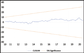
Figure 3 suggests that parameters of the model are stable. Further, the results for RESET test suggest that RESET statistic is 1.97 with p value = .1436, which is more than .05, which indicates that there are no misspecifications present in the model.
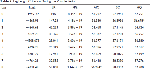
The lag value used in the model is selected as 1 according to the SIC as shown in Table 7.
Lag Length Criterion During the Volatile Period.
The VAR results depicting the trading behaviour of the institutional investors during the calm period is given in Table 8.
VAR Results During the Volatile Period.
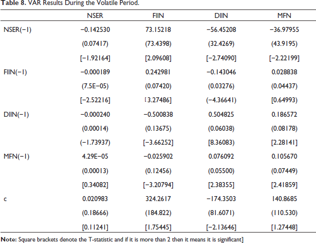
The VAR result suggests that NSER has a significant negative relation with DIIs and MFs while a significant positive relation with FIIs. Further, FIIs and DIIs follow opposite trading strategies and MFs follow a strategy similar to DIIs. It can also be noticed that the lag value of mutual funds is capable of influencing the trading patterns of the other two investors significantly.
Further, we applied IRF to examine the response of one variable to the changes in other variables. Figure 4 shows the impulse response function during the volatile period.
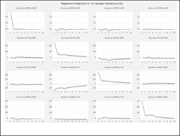
Figure 4 depicts that FIIs react positively to the market returns and adopt an opposite trading strategy to DIIs and MFs. Further, DIIs respond negatively to the market return and FIIs while positively to MFs. Lastly, MFs respond negatively to FIIs and positively to DIIs. Further, we employed variance decomposition analysis to find out the cause of the variance in each of the endogenous variable.
Table 9 shows the result obtained by applying VDA during the volatile period. It indicates that the variance in the market return is explained majorly by FIIs. Further, FIIs are influenced by DIIs and market return. Domestic investors are highly influenced by the trading pattern adopted by FIIs followed by market return. Lastly, the variance caused in the net flows arising from MFs is explained by domestic investors and market return in an equal proportion approximately. Therefore, FIIs follow a positive feedback trading strategy, whereas DIIs and MFs follow a contrarian trading strategy.
Variance Decomposition Analysis During the Volatile Period.
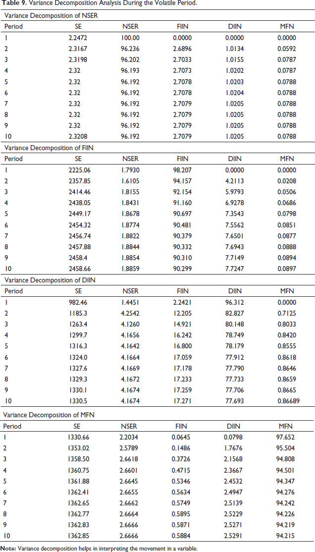
Thus, we can conclude that the interdependency of the institutional investors among themselves and on the stock market returns increases during periods of high volatility in the Indian stock market compared to calm periods.
The results indicate that FIIs follow a positive feedback trading strategy, while DIIs and MFs follow a contrarian feedback trading strategy in both the models. Thus, we accept all the alternate hypotheses as the results found in this study align with the formulated hypotheses. FIIs act as destabilisers in the Indian stock market, and DIIs and MFs act as stabilisers in the Indian market (Bansal & Rao, 2018; Chauhan & Chaklader, 2020; De & Ghosh, 2019; Dhingra et al., 2016; Raphael & Jacob, 2021; Sathish, 2020).
It is startling to compare the role played by MFs in both the subperiods. During the calm period, mutual funds were passive investors (Bhanumurthy & Singh, 2013; Bose, 2012). On the contrary, MFs increased their investments and significantly influenced trading patterns of the other two institutional investors in the volatile period (Lakshman et al., 2013). Therefore, we can conclude that MFs were looked as an important and influential category of investors during the period of high volatility. The herding behaviour during the volatile period could be sensed in the present study, which is corroborated in the commodity market as well (Kumar et al., 2021). In other words, the interdependency or herding behaviour increases during the bearish sentiments in volatile times as found by Sibande et al. (2021) in the currency market. This simply means that investor behaviour during volatile period remains the same irrespective of the type of market.
To conclude, in the present study, we have observed similar trading strategies followed by each of the three institutional investors in both the sub-periods. In other words, FIIs are positive traders while DIIs and MFs are contrarian traders in both the volatile and calm periods as distinguished in the study. However, some significant details regarding the interdependency/herding among the behaviour of institutional investors are observed in the volatile period when compared to the calm period, and hence, we can say that the structural break helps to enhance the forecasting and accuracy of the model as opposed by Boot and Pick (2020).
Conclusion
The present paper deals with examining the trading behaviour exhibited by the three most important institutional investors in the Indian stock market during the calm and volatile periods created through structural breakpoint. The trading behaviour of the institutional investors remains the same in both the subperiods, but the magnitude and their relation among themselves change significantly. FIIs adopted a positive feedback trading strategy, while DIIs and MFs followed a contrarian feedback trading strategy (Bose, 2012; Kim & Wei, 2002; Reis et al., 2010; Srinivasan & Kalaivani, 2015).
Implications
This study has some practical implications for policymakers and investors. First, it will help the concerned authority to understand the impact of market crash on the trading behaviours of the institutional investors and thereby their sentiments in the Indian stock market. Second, the retail investors will be benefitted to a great extent. They will be in a better position to decide whether to follow FIIs or DIIs. The present study limits itself in analysing the trading behaviour of investors in the stock market only. Future researchers can analyse the behavioural pricing in commodity or currency markets with respect to different categories of institutional investors and can take the support from leading research papers like Kumar et al. (2021) and Sibande et al. (2021).
Footnotes
Declaration of Conflicting Interests
The authors declared no potential conflicts of interest with respect to the research, authorship and/or publication of this article.
Funding
The authors received no financial support for the research, authorship and/or publication of this article.