
Abstract
The empirical relationship between tourism inflow and international trade has been explored during recent years, supporting the argument that international tourism inflow promotes international trade between countries. However, the impact of international tourism inflow on agricultural exports has been neglected within standard agricultural trade models such as agricultural exports function and gravity model. The main aim of the article is to provide theoretical and empirical evidence that international tourism inflow matters for agricultural trade. The study uses an agricultural export demand function and augmented gravity model to examine the impact of tourism inflow on agricultural exports of India from the top 10 importing countries for the period 2000–2019. The agricultural trade model is estimated using random effect and fixed-effect model. To overcome the problem of panel heteroscedasticity and autocorrelation, it uses the panel corrected standard error model. Further, potential endogeneity is treated by using a 2SLS model. The empirical evidence confirms the significant and positive impact of tourism inflow on agricultural exports of India.
Introduction
India’s integration into the world economy should be analysed through its performance in the world economy, especially its contribution to total agricultural trade (Barma, 2017). The value-added of total agricultural and allied in the country’s gross domestic product (GDP) has come down from 21.6% in 2000 to 16.6% in 2019 while still employing 42.6% in the labour force (Worldbank database, 2021). The gap between the percentage of the labour force and the percentage of income generated in the agricultural sector poses stress and inequality in the economy. Increasing the total value added in the agricultural sector will contribute to the overall growth economy and also re-establishes the income balance within the economy. This objective can be realised through international trade of agricultural exports. However, even after 30 years of liberalisation, India’s contribution to world trade is merely 1.7%, out of which the agriculture sector is contributing about 11.5% in 2019 (WTO, Country Trade Profile, 2021). The share in agricultural exports rose from 1% in 2000 to 3.6% in 2019 (compiled from WITS, World Bank Agricultural Trade Data). Clearly, Indian agricultural exports show a massive growth relative to the world share of total agriculture exports. In 2019, India’s top 10 agricultural imported countries contributed about 49% of total agricultural exports. Among these top 10 importing countries, USA contributed 12.56%, China (7.7%), Iran (6.21%), Vietnam (5.8%), UAE (4.65%), Bangladesh (3.54%), Nepal (2.35%), Malaysia (2.26%), Indonesia (2.01%), and Sri-Lanka contributed 1.15% in 2019 (compiled from UNCOMTRADE, 2021).
From the point of trade policy formation, there is a need for a comprehensive study on various determinants of agricultural exports in the face of the highly changing and competitive world market. Various studies have focussed on the impact of trade on economic growth (Modak & Pallabi, 2014), poverty and inequality (Topalova, 2010), productivity (Mahadevan, 2003), determinants of bilateral trade (Srinivasan & Archana, 2009) and mainly on efficiency (Barma, 2017) among others. The present article will add literature by employing the role of tourism inflow on agricultural exports.
While much has been researched about the success or lack of India’s international trade front, very little work has been done to study the role of tourism inflow on agriculture trade. India is a large market for international tourism. India is gifted with more than 500,000+ heritage sites, and about 30 (out of 38) cultural heritage are world heritage sites identified by UNESCO (Niti Aayog, 2019). In addition, improving infrastructure and developing India’s thematic tourism (religion, nature, history, etc.) are further reasons for increasing tourist demand (India Brand Equity Foundation report, 2018). India is ranked 32 in the tourism competitiveness across the world. Its contribution to GDP was US$ 121.9 billion in 2020 and is expected to reach US$ 512 billion by 2028. During 2014–2019, India witnessed huge growth in jobs creation (6.36) due to tourism inflow, followed by China (5.47million) and the Philippines (2.53) (World Economic Forum, 2019).
Researchers have been growing interested in knowing the relationship between tourism inflow and international trade in recent years. Empirical studies have tested relations using co-integration and causality techniques (Khan et al., 2005; Kulendran & Wilson, 2000; and more recently Santana-Gallego et al., 2016). The main conclusion of studies is that there exists causality between tourism inflow and international trade, and it happens mostly that tourism stimulates international trade. However, despite this evidence, the impact of tourism on international trade (particularly on agricultural trade) has been neglected within the international trade models like export function or gravity model (Santana-Gallego et al., 2016).
In literature, various channels have been suggested through which tourism inflow affects international trade. First, represents the preference channel indicating that tourists present important and costless information on foreign demand preferences, which helps the domestic firms produce new goods for the international market (Marrocu & Paci, 2011). Brau and Pinna (2013) present that tourism provides information on local products and foreign preferences. The second involves the transaction costs channel indicating that successful tourism trips promote exports and imports in subsequent periods (Kulendran & Wilson, 2000). Third represents the market size channel showing that tourists purchase food, transportation, and other goods and services in a foreign country (Khan et al. 2005).
From various literatures, tourism inflow can be introduced in the agricultural trade model by recognising that tourism inflow reduces both variable and fixed costs. Trade variable costs represent the transportation costs and tariffs on trade. On the other hand, fixed trade costs represent foreign standards, regulatory environment, and shipping rules set up by foreign agencies (Melitz, 2003). Tourism inflow reduces the trade costs by improving the knowledge about business habits and foreign culture. Further, it helps to learn foreign languages and therefore helps to make foreign easier. Concerning fixed trade costs, tourism reduces the information deficiencies about favourable contracts and production. It provides the necessary information to domestic firms that can be exploited to develop a positive impact on efficiency level (Marrocu & Paci, 2011). Direct contact between local markets and tourists presents a cheap way to supply particular goods than simply promoting international advertising (Khadaroo & Seetanah, 2008). Further, investment in transport and infrastructure decreases trade costs (Kalirajan, 2011).
Figure 1 reveals that India’s tourist inflows and agricultural exports to the top 10 importing countries are positively correlated. To understand the nature of the relationship, we include tourism in the agricultural trade model by recognising that tourism could reduce trade costs and therefore increase agricultural exports. The agricultural trade model of paper is developed using the agricultural export function and gravity model. The agricultural trade model is estimated using random effect and fixed-effect model. To overcome the problem of panel heteroscedasticity and autocorrelation, we use the panel corrected standard error (PCSE) model. Further, we treat potential endogeneity by using the 2SLS model.
Correlation Between Tourism Inflow and Agricultural Exports from the Top 10 Importing Countries.
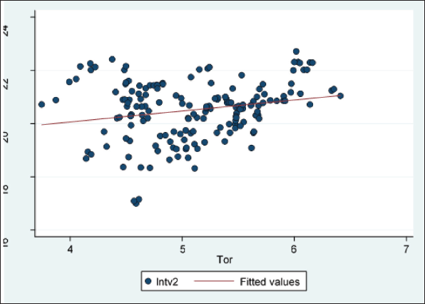
Correlation Between Tourism Inflow and Agricultural Exports from the Top 10 Importing Countries.
The structure of the article is follows as: Section II presents the findings of various previous papers. Section III discusses the theoretical model. Section IV presents the empirical estimation of the agriculture trade model and dataset used in the article. The empirical results of the article are discussed in Section V. Lastly, Section VI concludes the article.
In recent years, researchers have been growing interested in knowing the various determinants of agriculture exports. Most research has been carried out either using the agricultural export function or the gravity model. The agricultural export demand function assumes that agricultural exports mainly depend on the income of importing country, relative export price level, and the relative exchange rate between exporting and importing country (Bahmani-Oskooee, 1986; Wilson & Takacs, 1979). An increase in the income of importing countries induces more spending on our exports and therefore, our agricultural exports will increase. At the same time, if the increase in importing country income is due to an increase in their production of import substitutes, our agricultural exports will decrease. A rise in relative prices means our agricultural exports are relatively more expensive and expected to fall. Further appreciation of domestic currency makes agricultural exports less attractive for importers, and agricultural exports fall. Numerous studies had estimated the export demand function, including Shiells et al. (1986), and Bahmani-Oskooee (1998) at the aggregate level. For agricultural exports, the empirical studies are very limited, including Khan (1975), and so on.
On the other hand, supporters of the gravity model explain agricultural trade in terms of Newton’s law of gravity by the attraction of two masses measured in terms of GDP or population of two countries and weakened by the distance between them (Tinbergen, 1962). The basic gravity model is augmented with many variables to test whether they are relevant for determining agricultural trade between countries (Martinez & Nowak, 2003). These include agricultural inputs, exchange rate, inflation, arable land, various regional trade agreements, and other bilateral trade costs like a common language, common border, colony, etc. Sohn (2005) estimated the gravity model of bilateral trade between Korea and its 30 importing countries. A study conducted by Hassan (2001) examined the potential of SAARC using the gravity model. Other studies that estimated the gravity model are Huot and Kakinaka (2007) and Andre and Joe (2008).
In recent literature, researchers have had a growing interest in examining the role of tourism inflow on international trade. Most of these researches have been carried out using the cointegration and causality test, and results have been found mixed (Santana-Gallego et al., 2016). Kulendran and Wilson (2000) examined the relationship between tourism inflow and international trade for Australia with its four importing countries and found that tourism inflow Ganger causes international trade. Further, Santana-Gallego et al. (2011) showed that inbound tourism promotes international in OECD countries. On the other hand, Fry et al. (2010) found bi-directional causality between tourism inflow and international trade between South Africa and 40 importing African countries. However, the relationship between tourism inflow and international trade has been neglected with standard international trade theory like the gravity model (Santana-Gallego et al., 2016). Viljoen et al. (2019) applied the gravity model to determine international trade to bilateral African tourism flows. El-Sahil (2017) examined the causal effect of tourist inflows on non-OCED and European exporters from 1995 to 2013 using the gravity model. The result of the study indicates that an increase in inbound tourism leads to an increase in exports of a differentiated product. Santana-Gallego et al. (2016) examined the role of tourism in determining trade using cross-sectional data of 195 countries in 2012. To address the problem of endogeneity, they used a set of instruments, including the logo of tourism inflow in 2011. Their results indicate that a 1% increase in tourism inflow increases agricultural exports by 9%.
Studies on the nexus between tourism inflow and trade have accounted for international trade on total goods and services but not agricultural exports. Furthermore, we have not come across a study done on India. Therefore, the present article aims to contribute to the literature by exploring the role of tourism inflow on the agricultural exports of India while accounting for both the agricultural demand function and gravity model.
Empirical Estimation
Wilson and Takacs (1979) used the following empirical estimation for agricultural export demand function:

where
An increase in world income induces more spending on imports and therefore our exports rises. If world income rises due to the increasing production of import substitutes, domestic exports are expected to decline because of the rise in world income. Exports are relatively more expensive due to a rise in the relative price of exports, and therefore elasticity coefficient of exports with relative export prices is negative. A rise in the nominal exchange rate (an appreciation of domestic currency) makes domestic exports expensive, and exports are expected to decline. Therefore elasticity coefficient of exports with the nominal exchange rate is negative. Cho et al. (2002) argued that the negative impact of the exchange rate is more significant in agricultural trade than other sectors of the economy. Cho et al. (2002) were later empirically supported by Sheldon et al. (2013).
On the other hand, authors like Pokrivčák and Šindlerová (2011) adopted the following gravity model to explain the flow of trade between countries or regions.
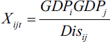
where
McCallum (1995) adjusted the basic gravity model for logarithm form and allowed adding supplementary variables as

where
By incorporating the variables of Equations (1) and (2), we built a model and added variable tourism inflow and fertilisers per hectare land as a determinant of agricultural exports. The modified agricultural exports demand function of India from the top 10 importing countries is:

where
The dependent variable used in the present study is the volume of Indian agricultural exports to the top 10 countries. We treat tourism inflow as exogenous flow. Tourist inflow impacts agriculture exports by reducing fixed and variable trade costs (Santana-Gallego et al., 2015). Variable trade costs include transport costs and tariffs (Melitz, 2003), while fixed costs are due to foreign standards and regulatory environment, set up distribution channels, and shipping rules specified by foreign countries. Tourism reduces the variable costs as it improves the knowledge about foreign culture and business habits. In addition, it stimulates the knowledge about foreign languages and therefore makes bilateral trade easy (Deardorff, 2014; Tadesse & White, 2010). Concerning fixed costs, tourism reduces the cultural distances and therefore reduces the costs associated with research of foreign standards (Santana-Gallego et al., 2015). Based on this, the expected marginal impact of tourism inflow on agricultural exports is positive.
For foreign income, we adopt conventional GDP (at 2015 prices) in US$ of importing partner representing the purchasing power and absorbing potential of importing countries. The theoretical framework of export function predicts either positive or negative marginal impact of foreign income, while the gravity model predicts a positive impact on agricultural exports (as discussed earlier). Fertilisers per hectare land is another conventional variable incorporated in the model to explain the relationship between agricultural productivity and India’s agricultural export flows. McArthura and McCord (2017) confirm that fertilisers are key to yield growth even with aggregate data and controlling factors like land–labour ratio and human capital. Therefore, the estimated coefficient of fertilisers has a positive sign.
To examine the effect of transportation cost, we include the variable of geographical distance between the capital cities of India (Delhi) and importing countries. Increasing distance between trading partners leads to higher transaction costs and decreases Indian agricultural exports flow. Therefore, the gravity model predicts a negative coefficient for the distance variable (Braha et al., 2017). On the other hand, lower transaction costs and lower transport costs are associated with neighbouring countries. Therefore, we expect a positive coefficient for variable agricultural exports with countries sharing a common border with India (Braha et al., 2017; Jansen & Piermartini, 2009). Further, the gravity model is augmented with dummy variable common language predicting effects of information and transaction costs through knowledge about home markets and languages. Literature suggests that common language may stimulate agricultural exports by lowering transaction and information costs and bringing their preferences for goods produced (see Braha et al., 2017; Parsons, 2005). In addition, we incorporate the dummy variable SAARC to capture the effects of trade liberalisation on Indian agricultural exports.
Following Braha et al. (2017), we used relative exchange rate, that is, a ratio of India’s exchange rate and importing country. We expect an increase in the exchange rate would appreciate Indian currency, and exports become costly. In such a case, an appreciation of domestic currency should decrease Indian agricultural exports. Therefore, as a result, we expect a negative coefficient of the exchange rate. Another factor influencing agricultural exports is price stability. To capture the impact of price stability, we include the ratio of household consumption prices of India and importing countries in the model. Therefore, we expect a negative sign for the coefficient of the ratio of household consumption prices. The description of variables of our model with data sources is in Table 1.
Variable Description.
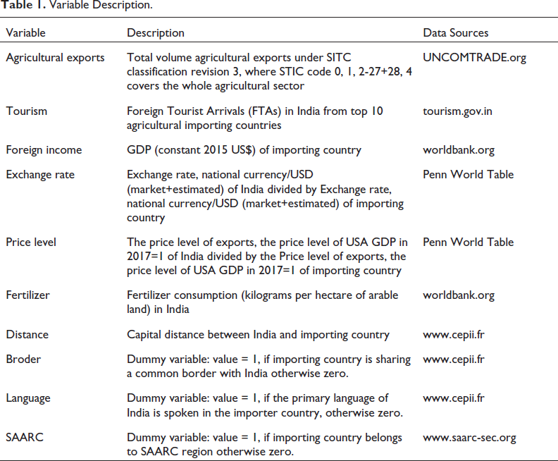
Specifically, we consider data for agricultural export flows from India to the top 10 importing countries from UNCOMTRADE database-based SITC classification. The tourism variable is obtained from the ministry of tourism of India. The distance variable, common border, common language are obtained from the GeoDist dataset. Data for foreign income and fertilisers per hectare land are obtained from the World Bank database; exchange rate and price of household consumption are collected from Penn World Table published by Groningen Growth and Development Centre. Lastly, the SAARC dummy variable is calculated from the official website of SAARC.
The present article examines the impact of tourism inflow on agricultural exports of India to the top 10 importing countries, namely, Bangladesh, China, Indonesia, Iran, Malaysia, Iran, Sri-Lanka, UAE, USA, and Vietnam. The study is based on secondary data and empirical in nature. It attempts to measure the marginal impact of tourism inflow on agricultural exports of India after controlling the core variables of agricultural export function. The study is restricted to 2000 to 2019 due to the lack of tourism inflow data of these countries before 2000. Further, the study is based on unbalanced data for countries/ cross-sections, Indonesia and Vietnam, starting from 2009, Iran (2006), and UAE (2006).
The research hypothesis of the present article implies that the tourism inflow coefficient is statistically zero, while as alternative hypothesis indicates that it is statistically positive. Tourism inflow reduces the variable and fixed trade costs and increases agricultural exports. Previous literature provides the positive values of the coefficient value of tourism inflow against the null hypothesis. The above-discussed model (Equation (3)) will check the coefficient value of tourism inflow on agricultural exports.
To verify the research hypothesis, parameters of Equation (3) are estimated using the random effect (RE) model, where it is assumed that country effects are uncorrelated with the independent variables. After that, parameters are estimated by the fixed effects (FE) model, which controls the correlation between explanatory variables and country effects. In the third step, the Hausman test is conducted to decide which model is best among random effects and fixed effects models. Further, the Wooldridge test is used to detect autocorrelation in panel data, and the Modified Wald test detects group-wise heteroskedasticity. In the presence of autocorrelation and heteroskedasticity, parameters are estimated using the PCSE model. PCSE estimates provide accurate standard errors, are less sensitive to outlier estimates, and are free from autocorrelation (Ikpesu et al., 2019). Also, the PCSE model performs better with dynamic heterogeneous panel data (Eboiyehi, 2017).
It is important to note that tourism has potential endogeneity, that is, tourism inflow between countries might also affect the agricultural trade between them. Various papers have applied a causality test (Kulendran & Wilson, 2000; Lin & Lee, 2002) and find evidence of a bidirectional relationship between tourism inflow and international trade. In addition, various authors like Awokuse (2002), and Dritsaki and Adamopoulos (2004) have found the bidirectional relationship between trade flow and economic growth. However, interpretation of the marginal impact of variables requires regressors as exogenous. Therefore, we need to address this endogeneity problem and attempt to correct it for more robust estimates.
There are two ways to remove the problem of endogeneity in panel data. One strategy is to use the lag of the right-hand side of variables. The past development of tourism and GDP can affect the current values of agricultural trade. Still, current values of agricultural trade will not affect the lag values of tourism inflow and foreign income. Therefore, we use the first lag of tourism and foreign income independent in RE, FE, and PSCE models. Bhattacharyya and Hodler (2010) and Bjorvatn et al. (2012) use a similar approach. The second strategy is to use the two-stage least square (2SLS) method. Following Farzanegan and Hassan (2016), we estimate parameters with 2SLS using two-year lags of tourism inflow and foreign income. To test the validity of instruments, we carry out three tests: Under identification test; Weak identification test; and Sargan statistic.
Empirical Results
We empirically test our hypothesis that tourism inflow increases agricultural exports in India by decreasing trade costs. Our estimation starts with RE, FE, and PCSE models. We use one lag of tourism inflow and foreign income to reduce the reverse feedback effect from these variables. The RE, FE, and PCSE are presented in Table 2. Hausman’s test confirms fixed effect model is more appropriate than the RE model. However, the Woodridge test confirms the presence of autocorrelation in panel data. In addition, the Modified Wald test detects group-wise heteroskedasticity in the FE model. Therefore, the PCSE model is more appropriate for the present study as PCSE estimates are free from autocorrelation and provide accurate standard errors.
Panel Regression Results.

Panel Regression Results.
Parenthesis in brackets shows P value; ***, **,* shows P value less than .01, .05 and .10, respectively.
The PCSE model confirms the negative and statistically significant marginal impact of tourism inflow on agricultural exports of India. The coefficient of tourism inflow means a one-unit increase in tourism inflow leads to a 0.0437 units increase in agricultural exports. Our results resemble the work of Santana-Gallego et al. (2016).
As predicted by our theoretical model, the relative price ratio exercises a negative marginal impact on agricultural exports. The law of demand justifies the theoretical justification. Increases in prices increase the costs and decrease the demand for agricultural exports. In addition, a sign of the coefficient of the relative real exchange rate is negative and significant as expected. The significance of relative exchange rate reiterates that depreciating real effective exchange rate enhances the competitiveness of agricultural exports in the international market (Love & Turner, 2001). Fugazza (2004) empirically found that 1% exchange rate depreciation could increase agricultural exports by 6%–10%.
The other determinant agricultural input use captured by fertilizer consumption per hectare of arable land has a significant and positive impact on agricultural exports. The estimated coefficient suggests that a one-unit increase in agricultural inputs leads to 5.22 units in agricultural exports. The result indicates the importance of using agricultural inputs to increase the production and productivity of high-value agricultural products and, therefore, increase India’s total agricultural exports. Kandiero and Randa (2004) also verify the positive coefficient of agricultural inputs.
The estimated coefficient of foreign income is negative implies negative elasticity of agricultural demand with foreign income. The economic theory may justify the negative coefficient that demand for agricultural products decreases with an increase in income, and people prefer to purchase high valued manufactured goods as income increases. However, the coefficient of foreign income is insignificant. The insignificance of this variable implies that foreign income does not increase the agricultural exports of India in the international market. Further, distance has an expected negative impact on the agricultural exports of India. The conventional gravity model justifies such an outcome. Distance is used as a proxy for trade costs. However, in our analysis, the estimated distance coefficient is positive and significant. These findings contradict the earlier studies (Osabuohien et al., 2019). Distance in the agriculture sector represents both transportation costs and a difference in cultivation and climatic conditions between trading countries. The farther away from the two trading countries, the greater differences in factor endowments and greater differences in agricultural products, which motivates more bilateral trade (Abdullahi et al., 2021).
Results of dummy variables (Common language and common border) of the augmented gravity model confirm the theoretical validity of the gravity model. The estimated coefficient of the dummy variable common language and the common border is positive and significant. Therefore, the result confirms higher agricultural export flow with countries with a common primary language and common border. Regarding the effect of trade liberalisation, the estimated coefficient confirms export diversion effects prevail from the foreign trade agreement with SAARC members. Accordingly, results induce a negative coefficient of SAARC but are statistically insignificant. The possible reason may be that free trade agreements in agriculture exports have delayed effects because of the asymmetric nature of foreign trade agreements. It may take several years to develop the export creation effect in the agricultural sector. Another possible reason may be the weak competitiveness of the Indian framers (for further explanation, see Braha et al., 2017).
Table 2 also presents the 2SLS estimation of Equation (3). We use 2-year lags of tourism inflow and foreign income as instruments. The set of other control variables is assumed predetermined. Our theoretical prediction and results of the PCSE model of the positive impact of tourism inflow on agricultural exports are supported by our 2SLS estimation. The positive effect of tourism inflow on agricultural exports is robust and slightly higher than the results of PCSE estimation. The positive estimated agricultural exports effect of tourism inflow is 0.4773 at the 1% level.
In 2SLS estimation, Anderson canon. corr. LM statistic of under-identification test strongly rejects the null hypothesis of under-identification. The value of Cragg–Donald Wald F statistics is higher than critical values and therefore rejecting the null hypothesis of weak instruments. Further, a P value of the Hansen J statistic fails to reject the null hypothesis of over-identification and confirms the instruments of study are valid. Therefore, the study results are robust and free from endogeneity and could be used for various policy implications.
The main contribution of the present article is to fill the gap left by theoretical and empirical research on the importance of tourism inflow for agricultural trade from agricultural export function and gravity model. From various literature on international trade, it may be concluded that tourism inflow could reduce variable and fixed costs through new information about markets provided by tourist visits, reduced cultural differences between trading countries, and improved infrastructural for tourist further facilitates agricultural trade. Thus in this article, tourism inflow is introduced as an independent variable by recognising that it could reduce the trade costs of agricultural exports. To address the impact of tourism inflow on agricultural exports of India, we use the unbalanced panel data of India’s top 10 agricultural importing countries over the period 2000–2019. Having discussed various econometric issues that ought to be considered, the PCSE model estimation results are preferred as the estimation technique yields robust results. In addition, to address the problem of endogeneity, we use the 2SLS model.
Our results support the theoretical prediction of a positive effect of tourism inflow on agricultural exports of India. Particularly, a 1% increase in tourism inflow increases the agricultural exports by 0.43%. These results are robust to the potential endogeneity between tourism inflow and total agricultural exports. Other findings based on agricultural export function and extended gravity model are; first, fertilisation per hectare of land in India stimulates agriculture exports. Second, India’s agricultural exports are negatively associated with the relative exchange rate and price ratio. Third, dummy variables of the common border and common language stimulate India’s agriculture exports. Fourth, the capital distance between India and importing countries positively determines the total agriculture exports of India. Lastly, foreign income and SAARC countries have an insignificant negative impact on the agriculture exports of India.
To facilitate the tourism inflow and promote their positive impact on total agricultural exports, India should focus more on tourism infrastructures, like better transportation, attractive tourist destinations, proper tax incentives, feasible hotels, and proper security arrangements with a free and peaceful environment for all potential tourists. Further, there is a need for firm supports from all sections of public authorities, private industries, and non-government organisations to attain sustainable growth in tourism inflows. All the economic actors must recognise the importance of this fast-growing industry and its positive impact on agricultural exports. Further, the Indian government should promote the latest inputs to improve agricultural productivity. In addition, depreciation of the Indian rupee against the currencies of importing countries would help to boost its agricultural exports. Lastly, maintaining low inflation reduces the costs and increases the demand for agricultural exports.
We admit that our study was limited to the impact of tourism inflow on India’s agricultural exports with only the top 10 importing countries. Therefore, the study results cannot be applied to agricultural exports as a whole. Future studies may add novelty to the literature by focussing on agricultural exports with more trading countries. Also, to incorporate the impact of tourism inflow on disaggregated product level agricultural data to examine the category of agricultural products most likely to be impacted by tourism inflow.
Footnotes
Declaration of Conflicting Interests
The authors declared no potential conflicts of interest with respect to the research, authorship and/or publication of this article.
Funding
The authors received no financial support for the research, authorship and/or publication of this article.