
Abstract
This article examines the disparities in poverty among the regions of Uttar Pradesh during the 2000s through a poverty decomposition exercise. While the poverty reduction from 2004–2005 to 2011–2012 is faster in the northern and southern upper Ganga plain, the reduction is slower in the eastern and southern regions. The poverty headcount ratio increases for the central region. While eastern and southern regions have higher real Monthly Per Capita Expenditure (MPCE) growth than the state average, the lower poverty elasticity in these regions caused slower poverty reduction. The southern and northern upper Ganga plain have high poverty elasticity causing a faster poverty reduction. This study finds that Uttar Pradesh’s central region faces a critical problem with increased Head-Count Ratio and declining MPCE. The differential change in poverty among the regions has also been analysed using the occupational pattern and landholding distribution among regions, both rural and urban areas.
Introduction
The post-reform period in India recorded a faster growth at the national and state level (Kumar & Subramanian, 2012). However, being a diverse country, the pattern of growth and poverty reduction among Indian states is uneven. There is vast literature on the backwardness and highest poverty ratio of the BIMARU 1 states, though the situation has improved in recent decades except for UP (Gaiha & Kulkarni, 2005; Kadekodi, 2020; Kathuria, 2008; Mohapatra & Giri, 2020). Uttar Pradesh (UP henceforth) is India’s most impoverished and populous state and accounts for the highest number of poor populations among the BIMARU states (Ojha, 2007; Pathak, 2010) and India. The annual change in poverty in UP is remarkably lower than the all-India figures during the recent period of 2004–2005 to 2011–2012 (Planning Commission, 2011).
The authors have found some aggregate-level studies on poverty in UP (Arora & Singh, 2017; Dubey et al., 2017; Mishra & Singh, 2020; Ojha, 2007; Pathak, 2010) and a few disaggregated studies (Pathak, 2010; Tiwari, 2014). However, there is a limitation to these disaggregated studies. UP has undergone significant administrative changes in the form of carving out the new state of Uttarakhand from UP in November 2000. Pathak (2010) and Tiwari (2014) have dropped the ‘Himalayan’ region from the erstwhile UP to compare it with the divided UP. While these are excellent academic works providing strict comparability among the four common regions of UP over a long period, the current policy relevance is moot. Arora and Singh (2017) have used the current classification, but their study is focused on identifying differential poverty incidence among regions of UP. To the best of the authors’ knowledge, no study has attempted to decompose poverty and inequality changes among all regions of post-reform UP. This study attempts to fill this gap by decomposing the poverty changes among all the regions of UP. It is also the first study to use the concept of poverty elasticity, as proposed by Besley et al. (2005) to explain the differential poverty changes among regions. Further, the change in the poverty incidence is explained by analysing occupational shifts and the size of operational holdings in regions.
The flow of the article is as follows. The second section presents a literature review. The third section presents the data and methodology used in the study. Section four deals with the poverty among regions of UP. Section five presents the poverty and inequality elasticity of growth among the regions of UP. Section six describes the decomposition of annual change in poverty among the regions of UP. Section seven presents the landholding patterns as a possible factor of regional differences in poverty changes, followed by a conclusion and policy suggestion in the last section.
Literature Review
Economic growth has a weak relationship with poverty alleviation (ODI, 2008). The extent to which growth decreases poverty appears to be associated with the poor’s participation in the growth process. Distribution created in the growth process is intrinsically related to economic growth and impacts poverty alleviation. It is vital to effectively execute income and asset redistribution policies for economic growth to alleviate poverty (Ahluwalia & Chenery, 1974). Poverty-eradication tactics evolved from basic growth to growth with income redistribution based on this concept. The concept of ‘pro-poor growth signified this new order’.
The issue of pro-poor growth has been studied at the country and cross-country levels (Sahoo, 2017; Son, 2004). The same has been studied at the state or regional level. Dubey and Tiwari (2018) found that inequality is the primary barrier to reducing poverty in the Indian states. However, this study is limited to the urban area of Indian states. A similar result has been found by the study of Dubey et al. (2017), which showed poverty reduction among the social group of Indian states.
Ojha (2007) found that poverty in rural UP had decreased by 6.56 percentage points during six years (1998–1999 to 2004–2005) in sample areas. This decline, however, was not unidirectional; instead, it was the outcome of two opposing movements. While some non-poor households fell into poverty, others who were previously poor could escape poverty. Mishra and Singh (2020) decomposed the poverty change between growth and redistribution effect for UP. They found that redistribution positively impacts urban Head-Count Ratio (HCR) due to the lower wage of casual workers and technical advancement. However, this study has not disaggregated the UP based on regions.
Tiwari (2014), using the Kakwani and Pernia (2000) decomposition method, found a positive effect of growth on poverty reduction in the central region during 2004–2005 to 2011–2012. However, our study differs from this; first, based on the method and second, based on regional classification. He has classified the UP region in four parts (to compare with the other round), whereas NSSO has been classifying the UP in five regions based on the agro-climatic zone. Thus, a study based on all the five regions of UP will be more relevant and informative for policymaking. Therefore, this study examines the pro-poorness of growth in all five regions of UP.
UP has been suffering from regional disparities and inequality for a long time, around six decades after independence (Diwakar, 2009). Arora and Singh (2017) show that UP has experienced an overall decline in poverty; however, inter-regional poverty represents an increasing trend in the level of deprivation in the rural Southern region (SR), in the urban Eastern region (ER) and both the rural and urban areas of the Central region. They also observed that there has been a decline in the inter-regional disparity in poverty. It can be further eliminated if there is a continuous decline in rural SR and urban ER poverty and a similar advancement in the deprived sections. Kozel and Parker (2003) observe three major challenges faced by the state while dealing with poverty. The first includes the expansion of economic opportunities, the second is concerned with the distribution of these opportunities among the poor (whether they can enjoy the benefits of these opportunities or not), and the third is to ensure the availability of a safety net to protect the very poor and to reduce the vulnerability. According to Srivastava and Ranjan (2016), the general development scenario has been influenced by poor governance and at the same time, ‘social justice’ oriented government has influenced socially inclusive development. As against this, Rasul and Sharma (2014) argue that the reason behind the low human development is the low level of financial assistance received from the Union government. Furthermore, political instability and class, caste, and ethnic-based social conflicts also added to the impoverishment of the state.
Data and Variables
The expert group methodology for the poverty line, as given by the Tendulkar Methodology (Planning Commission, 2011), has been used to compute the HCR, poverty gap (PG) and squared poverty gap (SPG) for the regions of Uttar Pradesh. The NSSO unit-level data on the ‘Consumer Expenditure Survey’ (CES) for the 2004–2005 (61st) and 2011–2012 (68th) rounds has been used. The MPCE figures are converted into real MPCE at 2004–2005 prices by using the poverty lines for both years. The National Sample Survey Offices (NSSO) classification of five regions based on agro-climatic zones in UP is used for our analysis. The percentage of poor (HCR) and the percentage of total poor, and the poverty risk among the regions have been calculated. The percentage of poor refers to the percentage of the population below the poverty line for a particular group, while the percentage of total poor refers to the contribution of a particular group to total poor. The percentage of total poor depends on the population of the particular group. The poverty risk of a group is the ratio of the percentage of poor of that group to the average percentage of total poor. The poverty risk greater than one implies the poverty for a particular region is higher than the average, and hence that region is more deprived. The annual rate of change in the percentage of poor among these regions is calculated and decomposed using the methodology described below. The landholding data of the CES is used to explain the regional difference in poverty among the regions of Uttar Pradesh, both in rural and urban areas.
Analytical Framework
Following Besley et al. (2005), the poverty reduction between two time periods in a region will be a function of both the poverty-growth elasticity

The value of
UP has been one of the backward states in India for decades. In terms of per capita income, it lags behind the national average and most states. It is in national headlines for hunger, starvation, malnutrition, death, and mass poverty. The state comes third after Bihar and Odisha in terms of the highest percentage of poor (Planning Commission, 2011). UP’s annual per capita income for 2019–2020 is estimated to be ₹70,418.00 compared to the all-India average of ₹96,536. The state has 71 districts classified into five different regions by NSSO: eastern, southern, central, southern upper Ganga plains (SUGP) and northern upper Ganga plains (NUGP) (the western region is divided into two parts: SUGP and NUGP). The ER currently has 27 districts, the central region nine districts, the SR 7 districts, the SUGP region has 18 districts, and the NUGP has 10 districts. UP has diversified geographical regions in terms of climatic condition, demographical characteristics and occupational distributions. Western (now SUGP and NUGP) and ERs contribute about 37% and 40% to the state population. Around 20% of the state’s population is in the Central region, and merely 5% in the SR. The population density of the SR is less than half that of the state, whereas the ER has the highest population density along with the lowest per capita availability of land (Srivastava & Ranjan, 2016). The NUGP and SUGP regions are the most developed regions of the states concerning economic prosperity. Their agricultural and industrial performances have made them leaders among the other regions.
UP has made considerable progress in reducing its poverty in 2004–2005 to 2011–2012 compared to 1993–1994 to 2004–2005. The rural poverty in the state has declined by 12 percentage points between 2004–2005 and 2011–2012. However, urban poverty reduction in the state has been relatively less impressive (about eight percentage points) for the same period. Compared to it, the pace of poverty reduction in India has been higher for rural and urban areas during this period (Figure 1).
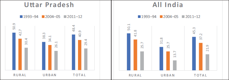
Table 1 presents the HCR, share in the total poor, and the poverty risk among the regions of rural UP. Though the HCR has declined for rural UP between 2004–2005 and 2011–2012, the eastern, southern, and central regions have HCR higher than the state average. The NUGP and SUGP have lower HCR than the state average. The ER contributes 50% of the rural poor in Uttar Pradesh, while 40% comes from the central and southern Ganga plain. The percentage contribution to total rural poor is lower among the northern Ganga plain and the SR. Though SR HCR (30.22) is higher than the state rural average in 2011–2012, the percentage share to total poor of this region is too low, 5.15%, which might be due to the lower percentage of the population in the SR. The poverty risk higher than one in the eastern and SRs implies a higher HCR and more deprivation than the state average. The northern and southern Ganga plains have a lower poverty risk than the state average. The central region recorded a rise in the poverty risk during the period.
Poverty Scenario Among the Rural Regions of UP.
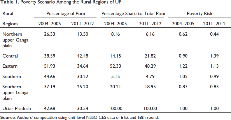
Table 2 shows that though the urban HCR has declined, the eastern, southern, and central regions have HCR higher than the state average. The urban HCR is lower among the upper Ganga plains, both the northern and southern. The central region recorded a rise in HCR, unlike every other region. The ER contributes 30% of the total urban poor in UP, while 31 comes from SUGP. The percentage contribution to the total poor is lower among the NUGP and the SR. Though SR HCR is higher than the state urban average in 2011–2012, the percentage share to total poor of this region is low 5.37% that could be due to the lower percentage of the population in the SR. The eastern, southern, and SUGP regions with a greater than one poverty risk imply a higher HCR than the state average and more deprivation. The northern and central regions have lower poverty risk than the state average. The central region recorded a rise in the poverty risk during the period.
Poverty Scenario Among the Urban Regions of UP.
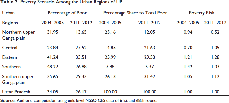
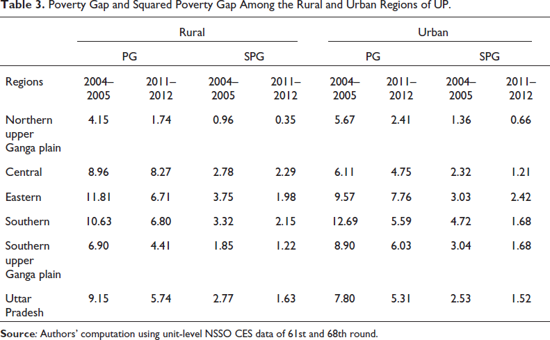
Table 3 shows the PG and SPG among the regions of UP for rural and urban areas for the year 2004–2005 and 2011–2012. The changes in PG and SPG are more or less similar to the HCR trends of Tables 1 and 2 for rural and urban areas. The fall in PG and SPG for all regions indicate the poor have moved closer to the poverty line, and inequality has fallen among the poor. Though the central region witnessed a rise in rural and urban HCR, the depth and severity of poverty have declined in this region.
Poverty Gap and Squared Poverty Gap Among the Rural and Urban Regions of UP.
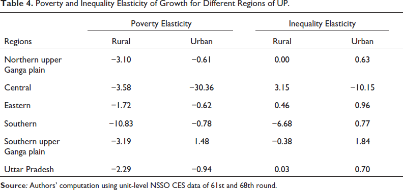
The relationship between growth and poverty can be established from poverty elasticity and growth and inequality from inequality-elasticity. The poverty elasticity is the ratio of relative change in poverty percentage between two periods to the relative change in MPCE between these periods. The inequality elasticity is the ratio of the percentage change in the Gini coefficient to the percentage change in MPCE between two periods. The value of the poverty elasticity will always be negative, implying that with a rise in MPCE, there will be a decline in poverty between the two periods. The poverty elasticity greater than one (ignoring the sign) implies that the poverty reduced faster than the rise in MPCE. Hence the greater the poverty elasticity, the better off the poor are from the growth process. If the poverty elasticity is lower than one, it implies that poverty reduction is lower than the rise in MPCE or income.
With a rise in MPCE or income, inequality might rise or fall, implying that the inequality elasticity between the two periods can be positive or negative. The positive sign of inequality elasticity implies that the growth in MPCE causes a rise in inequality which only benefits certain upper-income strata, while the negative sign of inequality elasticity implies a rise in MPCE leads to a reduction in inequality, implying that the lower strata has benefitted more than the upper-income groups.
Table 4 shows the poverty and inequality elasticity among regions of UP between 2004–2005 and 2011–2012 for the rural and urban areas. The poverty elasticity in rural areas is higher in the southern and central regions for the urban areas. The inequality elasticity is also negative and too high among these two regions in rural and urban areas, respectively. The higher poverty elasticity might be due to the anti-poverty programmes like MNREGA and the rise in public spending and spending on several welfare schemes, and reduction in inequality among these two regions, which is faster than the other regions. The poverty elasticity in the ER is too low both in rural and urban regions and is lower than the state average. The HCR in this region is also higher than in the other regions. The decline in HCR in the ER is slower than in other regions showing the ER as more deprived. Though the mean MPCE growth of this region is higher than the state average, it is the rise in inequality that is offsetting the poverty reduction in the ER of the state. The ER of the state remained more deprived. It recorded both a rise in MPCE and the rise in inequality over the period, which offset poverty reduction. The poverty elasticity in this region is negative but very small, implying a rise in MPCE causes a small reduction in poverty. The SR though witnesses a negative elasticity in the rural regions records a positive elasticity in the urban regions.
Poverty and Inequality Elasticity of Growth for Different Regions of UP.
Poverty and Inequality Elasticity of Growth for Different Regions of UP.
The inequality elasticity is positive in rural and urban UP, implying that the growth in MPCE causes a rise in inequality. Inequality-elasticity is negative for the rural SR and SUGP, whereas it is positive for the rest of the regions. The rural central region witnessed a high positive elasticity, implying a higher rise in inequality with a rise in MPCE during this period. In the urban regions, the central region witnesses a high negative inequality elasticity and elasticity is positive for the other regions of UP. While the rural areas of the central region witness positive inequality elasticity, the urban region witnesses a negative elasticity. Hence with growth in the central regions the rural area records a rise in inequality while the urban area records a fall in inequality. The ER, which witnesses a lower poverty reduction, witnesses a positive elasticity showing a growth in MPCE causes a rise in inequality offsetting the poverty reduction.
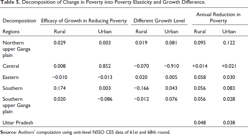
We have used the Besley et al. (2005) method to decompose annual changes in poverty to make a comparative analysis of poverty reduction among the regions of UP and the state average. As each region has different growth in MPCE and different poverty elasticity than the state average, the annual change in poverty among the region can be decomposed into the annual change in poverty in the state, difference in poverty elasticity between the state and the specific region, and difference in MPCE growth of a region with the state average. The methodology is explained in the data and methodology section of the article.
Table 5 compares the poverty elasticity and growth level of different regions with the state average in rural and urban regions. The NUGP witnessed a faster reduction in poverty among the regions, while the central region witnessed a rise in poverty HCR. The annual change in poverty among the regions can be decomposed into the average change in poverty, elasticity, and growth level. In the rural areas, the poverty elasticity is higher in the northern Ganga plain than the other regions and the state average, while the ER witnesses a lower poverty elasticity than the state average. At the same time, the growth in MPCE is higher in the eastern state and NUGP than in other regions, and the state average and the other regions witnessed a lower growth in MPCE than the state average. The high growth in MPCE and high poverty elasticity in the northern Ganga plain cause a faster poverty reduction. While the ER records a higher growth level, the lower poverty elasticity of the region causes a slower reduction in poverty in this region. Similarly, though the poverty elasticity is higher in the SR, the slower growth in MPCE causes a slower reduction in poverty in the rural areas.
Decomposition of Change in Poverty into Poverty Elasticity and Growth Difference.
Decomposition of Change in Poverty into Poverty Elasticity and Growth Difference.
In the urban UP, poverty reduction is higher in the northern Ganga plain followed by southern, eastern and SUGP regions. In contrast, the central region witnesses a rise in poverty. Even though the poverty elasticity of the central region is higher than the urban UP average, the growth in MPCE of the former is too low compared to the urban UP average causing a rise in annual poverty. The urban area of the NUGP records MPCE-growth higher than the urban state average, which, coupled with a high poverty elasticity, caused a faster poverty reduction. The SUGP has poverty elasticity lower than the state average and growth in MPCE higher than the state average, causing poverty reduction. The SR has high poverty elasticity and high growth in MPCE than the state urban average, causing a faster poverty reduction. In contrast, the urban area of the ER records a high growth in MPCE and lower poverty elasticity than the state urban average causing a slower poverty reduction. The NUGP region witnesses a higher reduction in poverty in both the rural and urban areas due to the high growth in MPCE and high poverty elasticity. The central region records a rise in poverty because of the slower growth in MPCE, and the ER witnesses a slower reduction in poverty because of slower poverty elasticity. Except for the central region, every region and the state itself has shown a decline in poverty between 2004–2005 and 2011–2012. We are trying to explore probable causes for an increase in poverty incidence in the central region.
The above discussion raises an obvious question: Why is there a difference in poverty changes among the regions of the state. Many factors might cause such regional differences. The distribution of landholding patterns and occupational patterns are among them. This section analyses these two factors to explain the regional differences in the state. The NSSO has classified the households in rural and urban areas into five and four categories, respectively, based on their occupation.
Change in Proportion of Household Types and Related Average MPCE: Rural Uttar Pradesh
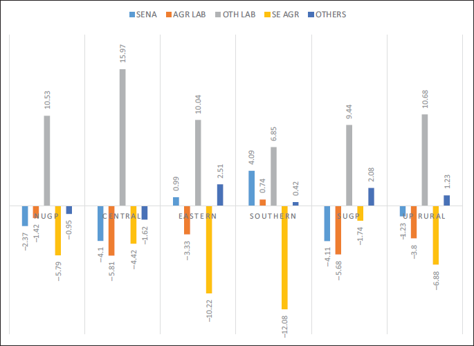
NSSO report ‘household types’ classified by the reported major source of income or livelihood during the last year for the household as a whole. Five household types are distinguished for the rural households by ownership or lack of physical or human capital, namely, (a) Self-employed in agriculture (SEA), (b) Self-employed in non-agriculture (SENA), (c) Rural agricultural labour (AL) and (d) Other rural labour (OL).
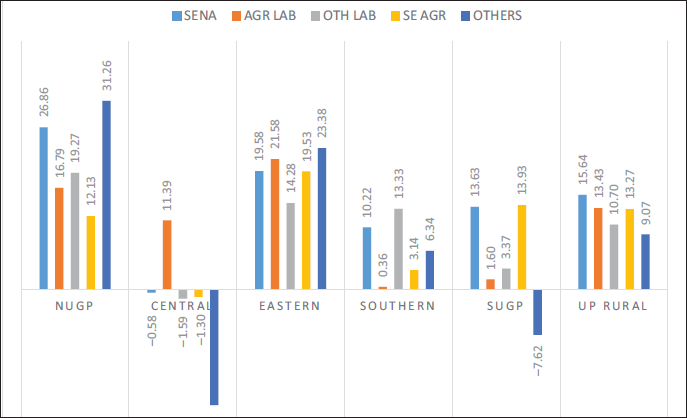
Figure 2 shows that among the regions of rural UP, the proportion of SEA and AL has decreased, and there is a rise in the population for the other labour category. It shows a structural transformation of employment where the population moves from farm to non-farm sector in rural UP from 2004–2005 to 2011–2012. The Central region is the only region to witness increased poverty in UP during this period. Even though there is a shift from rural farm to the non-farm sector, the average real MPCE has declined for every household type except AL between 2004–2005 and 2011–2012 (Figure 3).
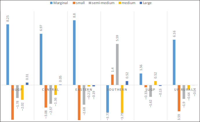
Rural Uttar Pradesh has witnessed a significant increase in marginal landholdings between 2004–2005 and 2011–2012. Except for the SR, marginal landholdings have increased while the medium, semi-medium and large holdings have decreased in all regions of UP. It indicates the growing fractionalisation of farms, possibly due to population pressure. The proportion of marginal landholdings has increased in the Central region. Agriculture has always played a significant role in the UP economy, and increasing fractionalisation of farms will affect the production and hence the income from the farm sector cause a rise in poverty in the state’s central region (Figure 4).
Change in Proportion of Household Types and Related Average MPCE: Urban Uttar Pradesh
For urban households, there are four categories, namely: (a) Self-employed households (SE), (b) Regular Wage and salaried earners (RWSE), (c) Casual labour households (CL), (d) others. Figure 5 shows the percentage point change in household types in urban UP, and Figure 6 shows the percentage change in real average MPCE for different household types between 2004–2005 and 2011–2012.
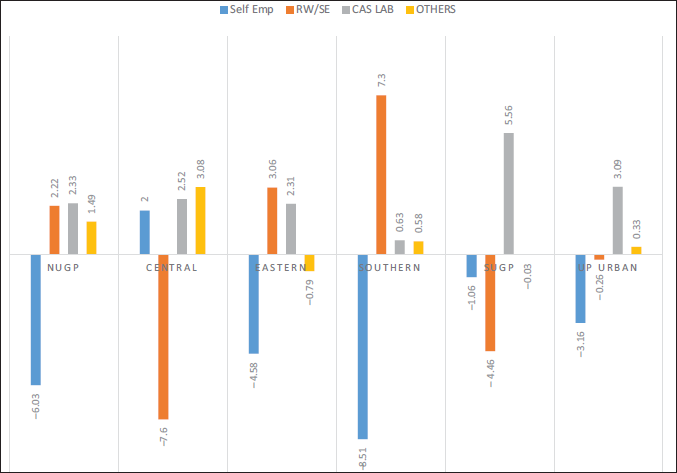
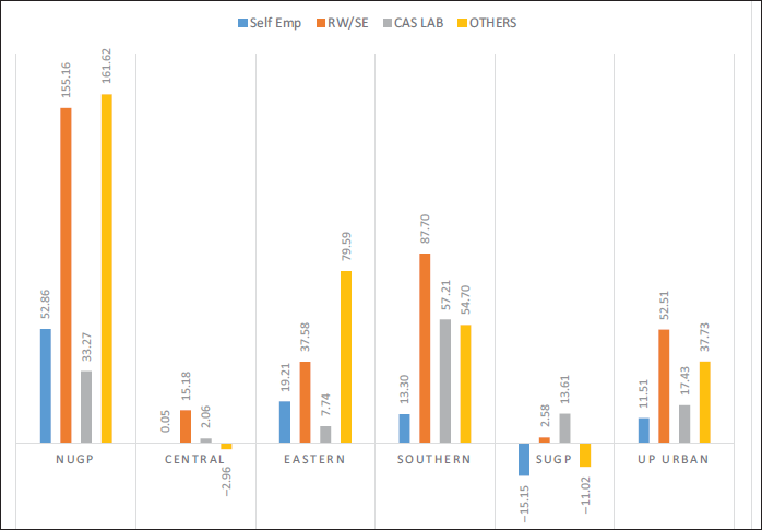
If we analyse the proportion of households based on the main occupation, we find that the proportion of self-employed households has increased between 2004–2005 and 2011–2012 in the Central region while that of the regular wage/salary earners (RWSE) has decreased. Self-employment is a vast spectrum ranging from petty self-employed to owners of well-doing household enterprises wherein the former dominates the category in terms of numbers. The real average MPCE of RWSE in the Central region in 2011–2012 was about ₹1446 while about ₹981 for the self-employed. It is also worth mentioning that the percentage increase in the real average MPCE of self-employed has been less than 1% while the average MPCE of the RWSE increased by about 15 per cent. A decline in the proportion of regular wage/salary earners coupled with the increase in self-employed could be one reason for the increase in poverty in the Central region between the two time periods. SUGP has also registered a decline in the proportion of households in RWSE, while the proportion of CL has increased. The average MPCE for this region has shown a 14% increase for CL and about a three percent increase for RWSE . It has decreased for all other household types between 2004–2005 and 2011–2012. It explains the increase in share of urban poverty in this region, though the overall poverty has declined.
Though UP achieved rapid poverty reduction in the post-reforms period, mainly the 2000s, the pace of poverty reduction is not the same among the regions. The NUGP region witnessed a higher poverty reduction in rural and urban areas due to the high growth in MPCE and high poverty elasticity. The central region recorded an increase in poverty because of the slower growth in MPCE. The ER witnessed a slower reduction in poverty because of low poverty elasticity despite high MPCE growth. The changing employment and occupational structure, land distributions and the respective earning potential could be responsible for the differential change in poverty among regions. The government should decline the disparity within the state and between the regions through more investment in the anti-poverty schemes and equal and fair distribution of income. There is a need to focus more on eastern, southern, and central regions for faster poverty reduction.
Footnotes
Acknowledgement
The authors would like to thank the editor and anonymous referees of the journal for their extremely useful suggestions to improve the quality of the article. Any remaining errors (if any) are ours. However, the usual disclaimer applies.
Declaration of Conflicting Interests
The authors declared no potential conflicts of interest with respect to the research, authorship and/or publication of this article.
Funding
The authors are thankful to BHU for the IOE Trans-disciplinary Grant received for the project.