Sage Journals: Discover world-class research

Abstract

The COVID pandemic seems to have raised the question, ‘whether existing supply chain (SC) disruption philosophies and strategies continue to remain valid?’. This article assesses the differences in the business scenarios pre-and post-COVID. The authors capture the mathematical and operational relationships amongst the relevant factors and propose a System Dynamics (SD) model to carry out the simulations. The approach considers the impact of the force majeure condition, that is, COVID period on individuals’ income, prices and demand of goods, cost of input and supply of finished goods. The results show that earnings may increase demand but, disruption in supplies of raw materials and finished products nullify the effect. On the other hand, even if flow returns to normal, reduced income affects normal goods businesses.

JEL Codes: R41

Keywords

COVID pandemic force majeure condition supply chain (SC) disruption demand system dynamics model policy and strategy experimentation

Introduction

On 30th January 2020, the World Health Organization (WHO) declared the COVID-19 as a public health emergency of internal concern (PHEIC). By the end of March 2020, affected countries in the EU, China and India were all under lockdown. At this time production stopped, movement of goods curtailed and the industry remained perplexed. The outbreak of this disease marked the beginning of a new era demanding re-thinking of business forms and management. It stopped the world from moving, and disrupted flow/network of flows of goods. The demand for shipping reduced and at the same time, the freight rates went up. This trend is unusual compared to the pre-COVID period. Figure 1 shows that before 2019 the volume of container traffic and shipping freight moved in a similar direction. That is, as the traffic grew, the rates also increased. Whereas, post-2019, the freight saw rise even when the traffic came down.

Figure 1.

Source: Created by author on data from Bloomberg.

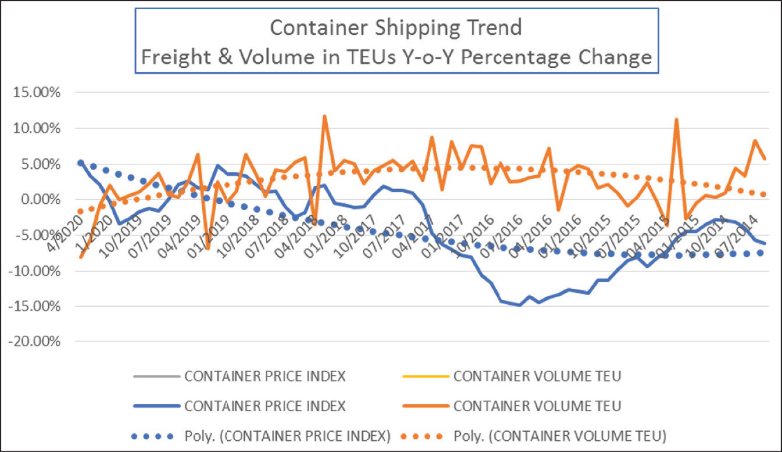
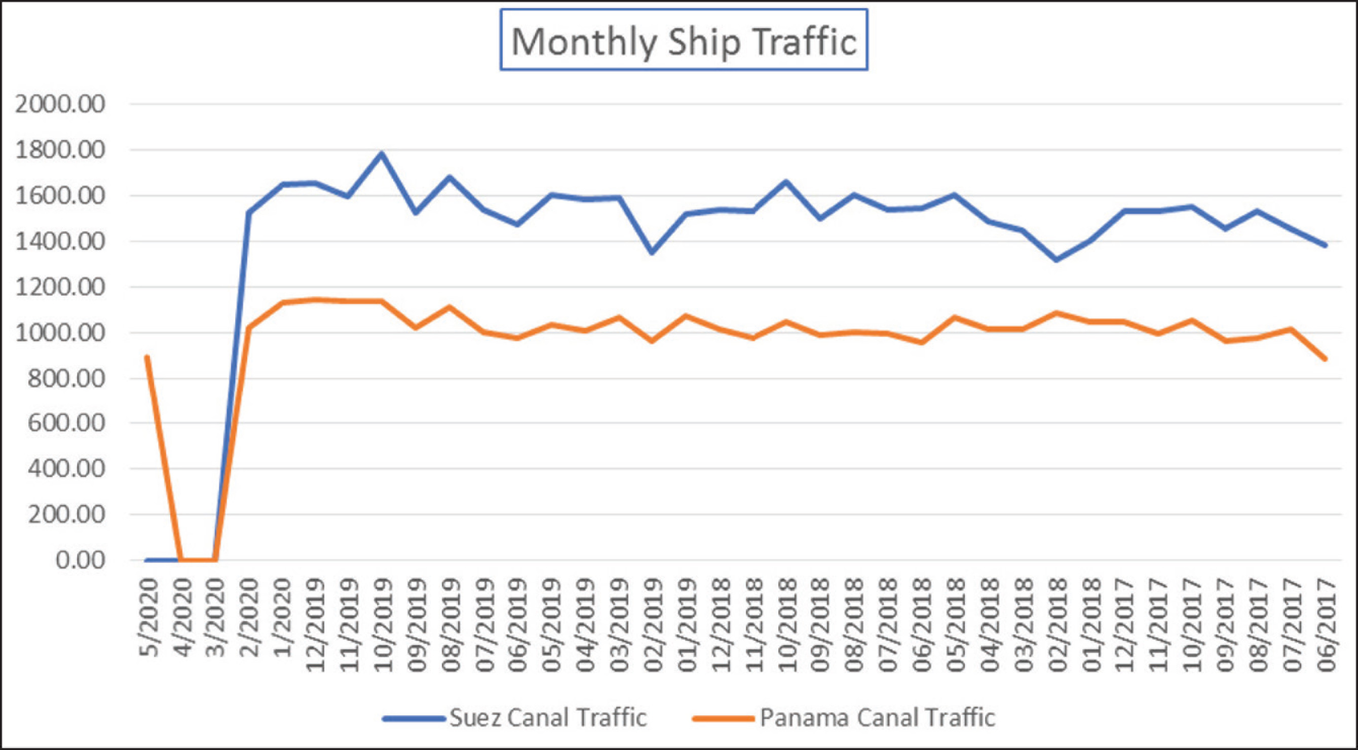
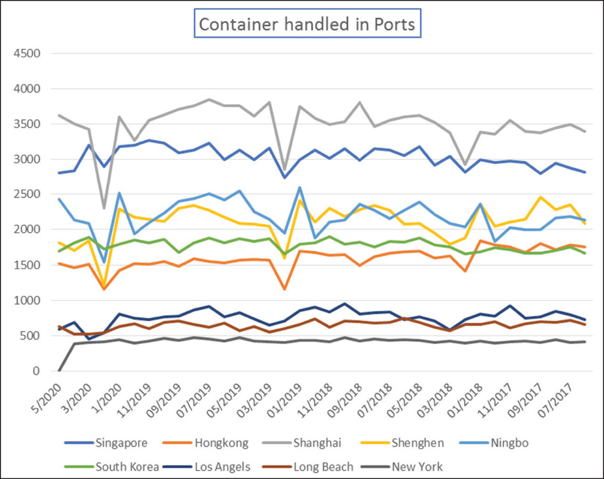
Figure 2 shows the drop in monthly vessel traffic across two crucial ship routes between January 2020 and May 2020. There was no vessel movement in March and April 2020. The container traffic in the world’s largest container port, namely dipped by 40 per cent in March 2020 compared to July 2019 (Figure 3). The port of New York handled zero traffic in May 2020. The total traffic in Chinese ports dipped by 39 per cent from September 2019 to February 2020.

Figure 2.

Source: Created by author on data from Bloomberg.

Although the basic definition of disruption of the supply chain remains unchanged, the previous researchers did not imagine this situation. This time the disruption is a global phenomenon.

Schmidt & Raman (2012) defined disruption as an ‘unplanned event that adversely affects a firm’s normal operations’. The instances of disorders showed regional focus such as natural-hazards, terrorist attacks and political disturbances. The present situation seems to have dis-proven the previous observation—‘disruptions have a significant impact on the least-developed country (UN, 2012)’. In June 2020, high-income countries such as USA, Italy, France, UK and Spain were the worst affected; following them are the emerging economies, namely, Russia, Brazil and India. Earlier studies discussed local or regional losses due to force majeure conditions, such as hurricane (reference on Katrina by Moynihan, 2009) or Tsunami (Koshimura & Shuto, 2015). They did not take into account the global disruption where no country or region gets spared. Therefore, in this article, the authors attempt to account for the impact of the pandemic on business, namely, its effects on income, price, demand, rate of production and supply of goods.

In this article, the authors reviewed the lean-agile-resilient and green (LARG) philosophy proposed by researchers till now, identified the shortfalls, explained the post-pandemic situation and offered a framework and a simulation model for policy experimentation under the global disruption. The model determines the causality between supply disruptions, economic recession and customer decisions.

Figure 3.

Source: Created by author on data from Bloomberg.

Ohio State University (2013) defined resilience (of an organisation) as its ability to survive, adapt and grow during disasters and catastrophic incidents. Cabral et al. (2012) observed that deploying the best practice and identifying key performance indicators (KPIs) is a complex problem when following the LARG paradigm. The authors advocated ‘systems for rapid response in emergencies and special demands’ as one of the LARG practices apart from strategic stock, and reuse of materials and packages. The KPIs remained inventory cost, order fulfilment rates and responsiveness to urgent deliveries. The existing model, thus, stood as shown in Figure 4.

The Existing Model

Figure 4 shows the causality of dimensions and variables under the LARG paradigm. It indicates that an increase in production lead time leads to an increase in lead time and cost, thus impacting the service level. The diagram demonstrates the need to enhance integration level and make supply chain (SC) resilient since this—reduces inventory level, causing a reduction in cost; and increases the service level. Inventory levels determine the leanness of an SC; lower inventory levels make organisations lean but impact the service level to drop. Thus, moving away from resilience and agility in SCM (Carvalho et al., 2011).

Figure 4 shows the conceptual diagram developed based on the System Dynamics (SD) approach, following the causality described by Carvalho & Machado (2009). In this causal scheme, it is possible to visualise how management characteristics affect performance indicators. A positive link indicates that the two nodes move in the same direction, that is, if the value of start node decrease, the value at the end node also decrease, when all else remains unchanged. In the negative link, the nodes change in opposite directions, that is, an increase will cause a decrease in another node, if all else remains unchanged.

Figure 4.

Source: Adapted from Carvalho & Machado (2009). Drawn using VENSIM software.

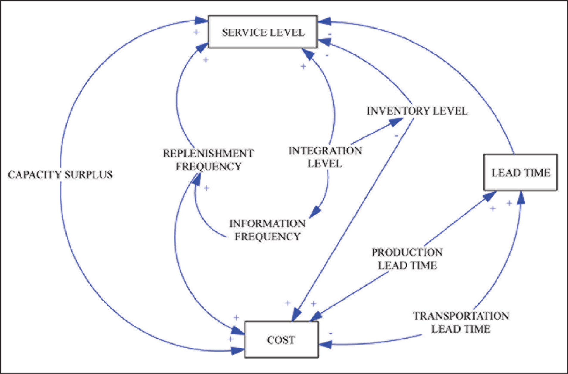
Inventory enhances service levels while at the same time, high inventory levels increase uncertainties (Van der Vorst & Beulens, 2002), making SC vulnerable to changes (Marley, 2006). More inventory leads to increased use of packaging materials and may lead to obsolescence, affecting the greenness of the SC.

The study by Cabral et al. (2012) revealed that the green aspect is the least significant factor in firms’ decision-making and reported that ‘systems for rapid response in emergencies and special demands’ is the most crucial aspect of practice for maintaining the SC service levels. These findings correlate the observations of Shakir Ullah et al. (2016)—SC managers give less priority to sustainability and affect ecology, leading to SC disruptions.

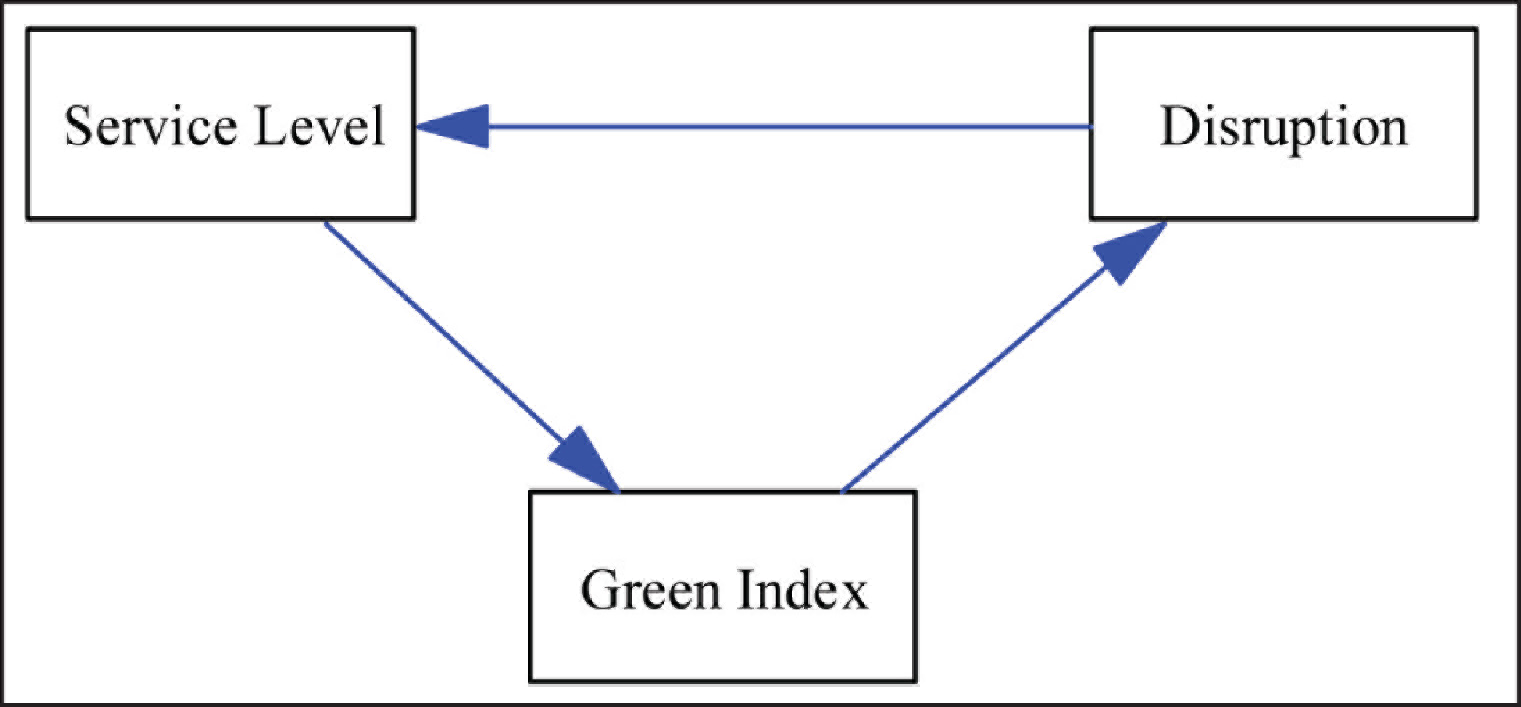
Considering this counter impact of the green state of business on supply chain disruption, the model described by Carvalho & Machado (2009) shown in Figure 4 needs to include the state variables: ‘Greenness’ and ‘Disruption’. Figure 5 shows the relationship between the disruption and green perspective.

Figure 5 signifies that greenness impacts the ecology leading to disruptions that, in turn, reduces the service levels. As the possibilities of disruptions increases, the inventory levels are increased to meet uncertainties, reducing the greenness of the firm’s SC.

Figure 5.

Source: Authors.

The Current Situation

The current (COVID-19) situation disrupts all the previously tested and conceptual models. The pandemic with the current economic slowdown and subsequent economic breakdown calls for re-orienting the supply chain decision models.

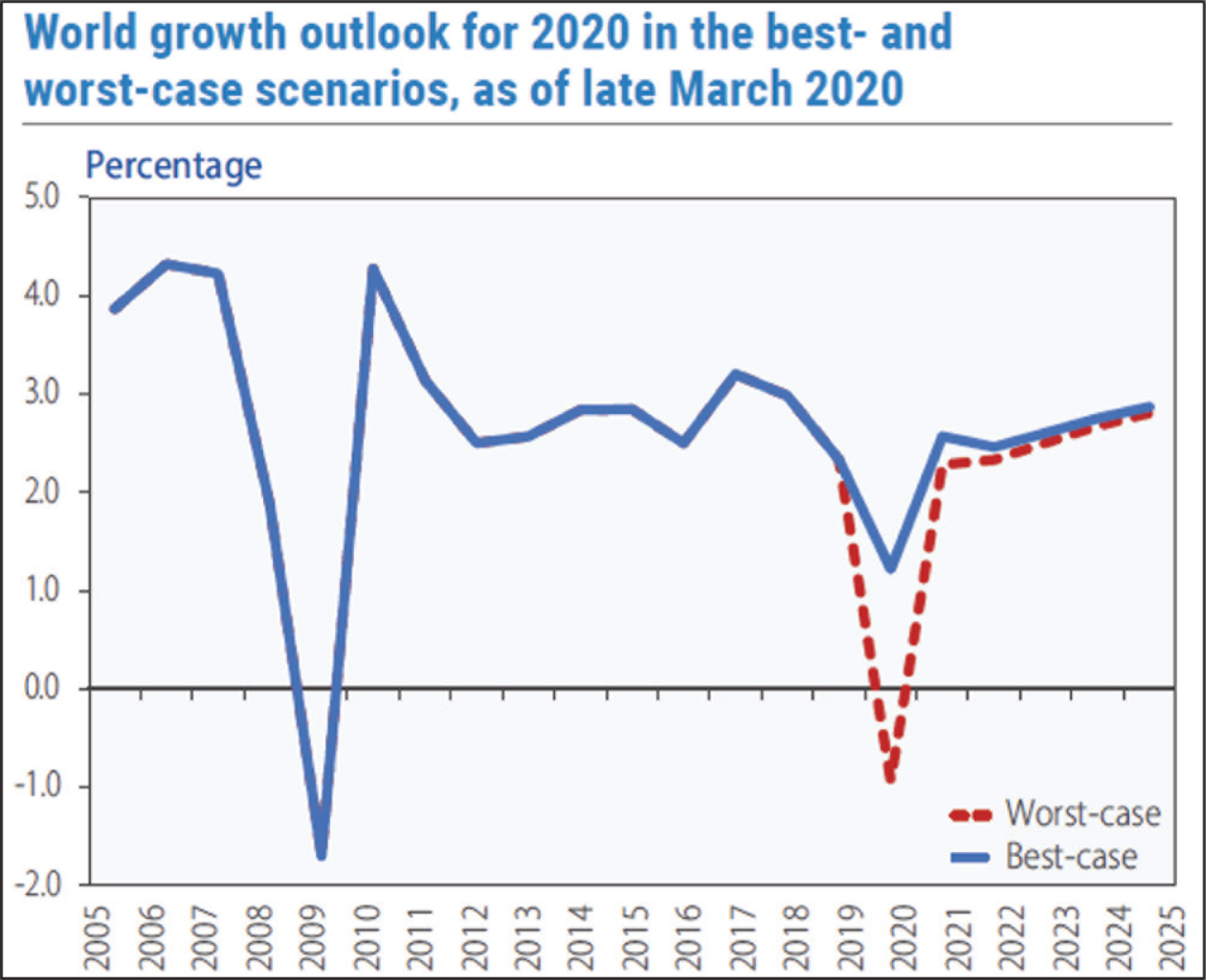
The data on the global economy and its projection (UN, 2020) shows that the economy can contract by 0.9 percentage and expected to bounce back to around 3 per cent after that (Figure 6).

Figure 6.

Source: Source: UN DESA.

Sinha and Dey (2018) observed that during economic slowdown inventory builds up, production slows down or stops and obsolescence increases. These outcomes impact working capital and finances leading to bankruptcy or scaling down of operations.

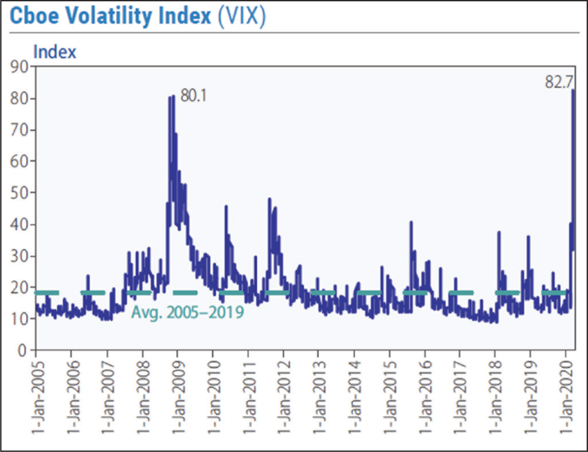
Figure 7 shows the volatility index indicating the market experiencing a high uncertainty level in the coming days. This uncertainty makes capacity-building difficult, along with the provisioning of funds.

Figure 7.

Source: Source: Cboe.

COVID-19 is likely to shrink global GDP by almost one percent in 2020. UN (2020) predicts a recession, and spillover of activities from developed to developing countries. These outcomes are likely to reduce incomes and impact both the manufacturing and the service sectors. The lockdown may create supply problems, and the extended restriction is likely to close down units followed by job losses. Thus, this transforms supply-side uncertainty to demand-side uncertainty. The closure of the businesses is likely to make people starve of food and essentials. UN estimates that in countries like Italy and Spain, the percentage of people who do not have enough savings to continue beyond three months is 27 and 40 percent. Closure of schools and their substitution with online classes is likely to create more educational divide in countries where school systems are still primitive.

Deloitte’s (2020) study reports a drop in industrial production by 9.1 per cent in April 2020, affecting the autos and steel firms. It expects the debt in the European Union to increase from 86 per cent to 100 per cent. In the US, unemployment increased and wage income dropped by 8 per cent, but the total income increased to 10.5 percent as the government transferred one-off transfer and increased the unemployment insurance. Nevertheless, the country witnessed a drop in spending as they preferred to save.

Thus, the current situation is all about income, educational and employment divide in nations. Regarding specific goods or products, one needs to see how it is affected by the price of goods and or income of buyers. Price-inelastic goods will continue to sell and bear demand subject to its logistics service, while price-elastic goods suffer when supply reduces due to closures and bankruptcies. The income-elastic goods, too, take a back seat as slowing down of the economy results in the lowering of individual incomes.

Besides, due to restrictions in the movement of people and goods, the inbound and outbound supply chains get disrupted. The world saw lockdowns or such restrictions, entirely or partially, since March 2020. The economy stalled, excepting some movement of essential goods. The oil price in the United States touched sub-zero in April 2020 (Web Desk, 2020). Shipping services suffered due to lack of demand and as passenger air services stopped, the change in ship crew got disrupted—the pending orders suffered due to the non-supply of inputs to production. The delay in the supply of orders and contraction of income led to the cancellation of orders.

Goods such as passenger cars demonstrate income elasticity (Sinha & Dey, 2018). Several authors (Dargay & Gately, 1997, 1999; Greenman, 1996; Medlock & Soligo, 2002; Lescaroux & Rech, 2008) link it to an S-shaped curve to depict the relationship between vehicle purchase and real per-capita income. Figure 8 illustrates the current situation. It captures sales of goods such as cars as the difference between the demand and the flow of goods to the customer. In pre-COVID situations, sales were the outcome of demand and supply. The illustration introduces a flow (rate of shipment) between the production and the orders. Previous works assume no restrictions on shipment of finished goods. Only the SC managers manipulated the time to ship or deliver with the inclusion of different modes of transportation. In this pandemic situation, transportation is allowed in different forms. For example, in India, under lockdown phase 1, only intra-state movements were allowed by road carriers, but goods trains continued to run; under lockdown phase 2, inter-state movements by road carriers were allowed and at present, that is, lockdown phase 2, inter-state airlines started operating. The shipping services were not stopped but suffered slow down due to port restrictions on crew transfer and halting of flights. Hub ports such as Singapore, Abu Dhabi and Shanghai halted crew transfer in March and April 2020. Besides, the flow of crew from the Philippines, the world’s largest crew provider, due to cancelled flights added on to the disruptions (Bloomberg, 2020).

Figure 8.

Source: Authors.

Thus the current situation envelops both the demand and supply shocks and one influencing the other.

Supply Chain Strategies: A Literature Review

Research on agile strategies for SCM dates back to the 1990s. It began with the recommendation of automation technology to achieve agility (Nagel & Dove, 1991; Goldman et al., 1995). Several authors worked on ways to implement agile SC (Sharifi & Zhang, 1999; Ismail et al., 2001) and advocated to view SCs as drivers of organisational competitiveness (Bowersox et al., 1998; Christopher, 1998). Authors in this field introduced the concept of demand chains to manage SC efficiently (Cox et al., 2000; Fine, 1998; Harland et al., 1999; Sharifi et al., 2002; Kehoe et al., 2004). Authors agreed that market sensitivity and responsiveness are the fundamental elements of an agile SC (Harrison et al., 1999; Christopher & Towill, 2000). They professed that there should be end-to-end integration for sharing information and process inter-connectivity. Van Hoek et al., 2001 stressed on responsiveness to volatile markets. The authors professed for customer involvement in the development of products followed by innovation to enhance responsiveness. Information on inventories becomes significant rather than physical inventory per se, and accordingly, SC infrastructure needs upgradations.

Ismail & Sharifi (2006) put forward the framework for agile SC (ASC) that accounted for market characteristics, including the business environment and prescribed the framework for design-for-supply-chain (DfSC). In DfSC, the SC strategy needs to capture customers’ voices (feedbacks), leading to identification and clustering of features and its alignment with internal and supplier capabilities.

Demand for normal-goods varies with income. As income increases, its demand goes up (Dargay & Gately, 1997, 1999; Greenman, 1996; Lescaroux & Rech, 2008). Researchers (Espey, 1998; Goodwin et al., 2004; McRae, 1994) have also shown that the long-run income elasticities vary with countries’ economies. It is higher for less developed countries than in developed countries and displays a temporal downward trend. The long-run income elasticities present more extensive variations: first they differ from one country to another, being almost systematically higher for less developed countries than for developed countries (McRae, 1994); second they display a temporal downward trend (Dahl, 1995; Espey, 1998; Goodwin et al., 2004). Normal-goods may demonstrate price elasticity (Neto, 2012; Wilkie & Godoy, 2001)

The previous studies proposed frameworks and SCM models based on the assumption that buffers and inventories, alternate sources and markets resolve the disruptions. There are significant works on optimising SC operations by trading off between redundancies or resilience and leanness.

In this article, the authors propose an SC framework that accounts for a drop in demand, restrictions in the inflow of inputs and outflow of finished goods. The authors suggest a SD model captures the sensitivity of goods on income and price, complete disruption in inflow and outflows, differentiated flows, both in and out of the manufacturing units. Thus, the authors propose a simulation exercise using VENSIM software to study the impact of different levels of uncertainties and disruptions.

The Conceptual Model

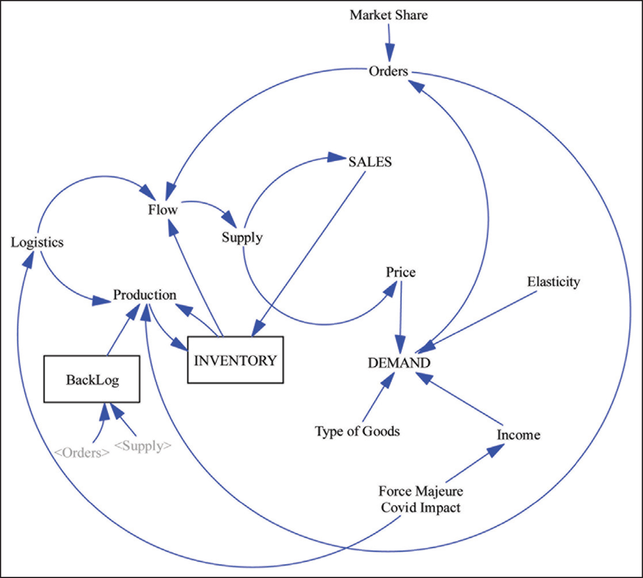
Figure 9 describes the conceptual model developed based on the understanding of the current situation and literature survey. The conceptual model helps in identifying the relationship between the auxiliary, rate and level variables. The study captures the variables and their relationships to develop the working simulation model, using the SD approach, for policy experimentation.

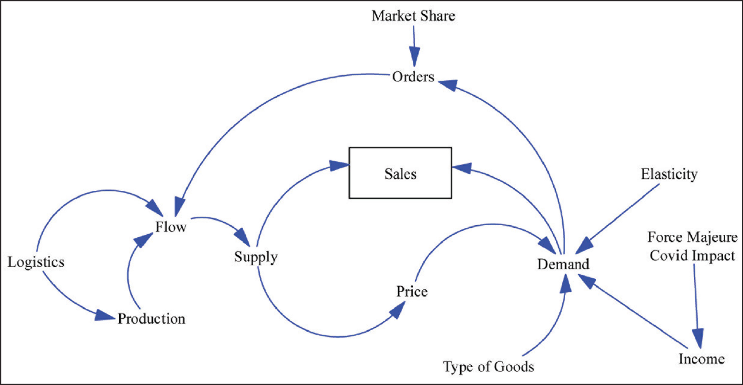
Figure 9 shows that there are two level-variables, that is, the inventory and backlog—these two variables, along with the order-rate, impact production rate. However, the rate of production is dependent on the flow of inputs and raw materials. In the current situation, there is a disruption in the logistics state and if the inflow of inbound materials is interrupted, the rate of production will be affected. Similarly, the flow of finished goods is dependent on the number of orders and the logistics state of the outbound supply chain. The sales will depend on the flow of finished goods and, in turn, will affect the inventory. The inventory builds up due to the difference between the rate of production and the rate of sales. The number of orders will depend on the type of goods, that is, either an essential good, not affected by either price of goods or income of consumers, or normal-goods that vary either with price or income. Thus the demand may vary with elasticity factors. The orders to individual companies will vary with their market share, that is, consumer preference. The backlog increases when the supply fails to meet the orders.

Figure 9.

Source: Authors.

Thus, the pandemic is not only affecting the income but also on the flow of goods. Figure 10 shows the causality of flow.

Figure 10.

Source: Authors.

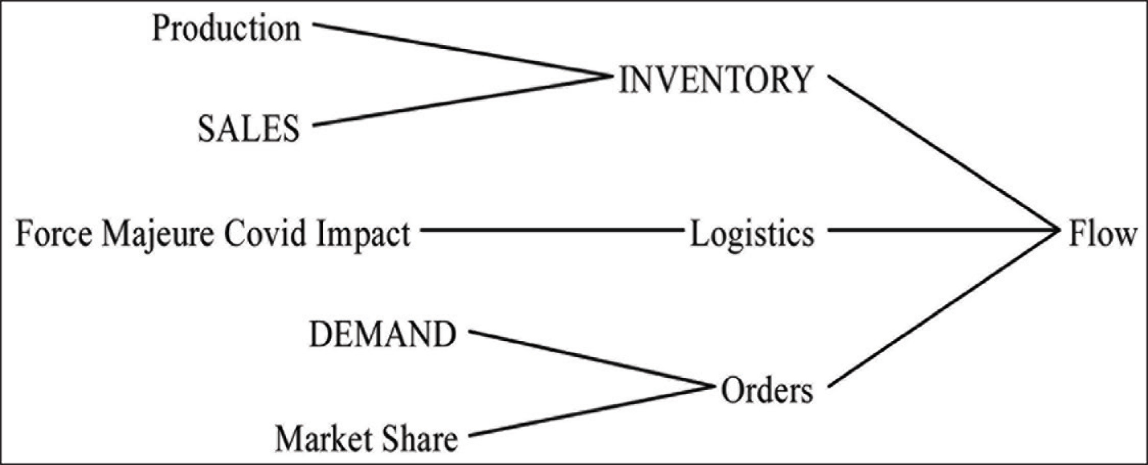
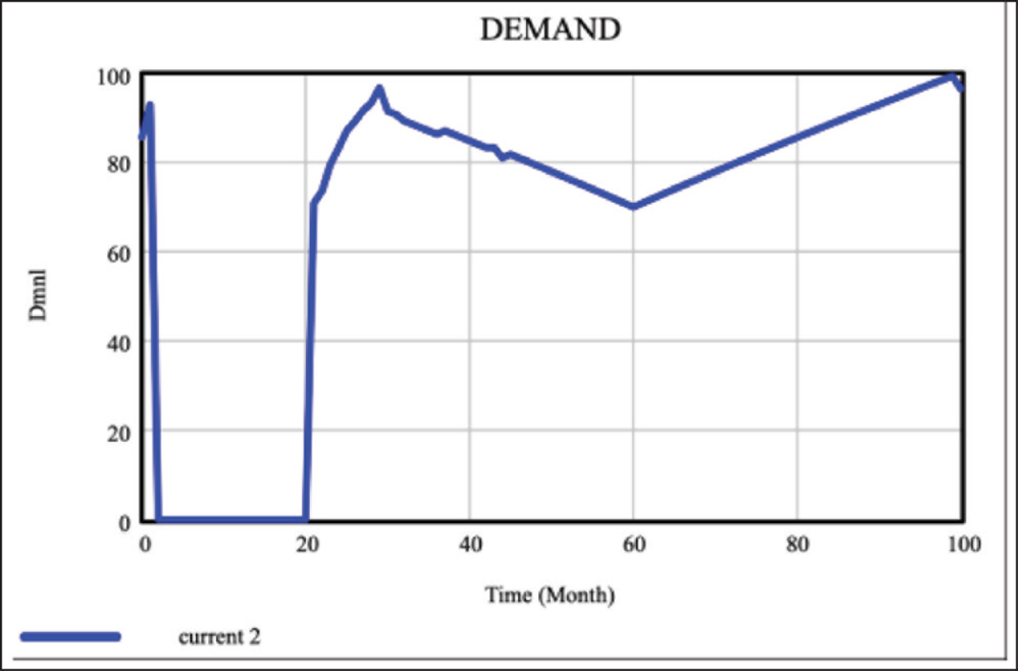
Figure 11 shows that the demand is affected by the types of goods and the elasticities (income and/ or price).

Figure 11.

Source: Authors.

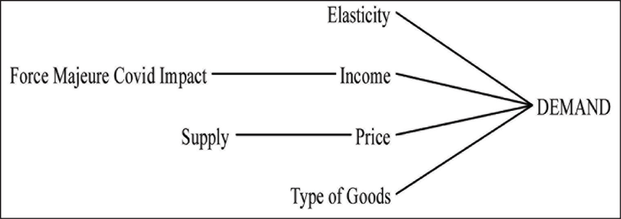
Figure 12 summarises the relationship between the economic trend and the inventory and backlog.

Figure 12.

Source: Authors.

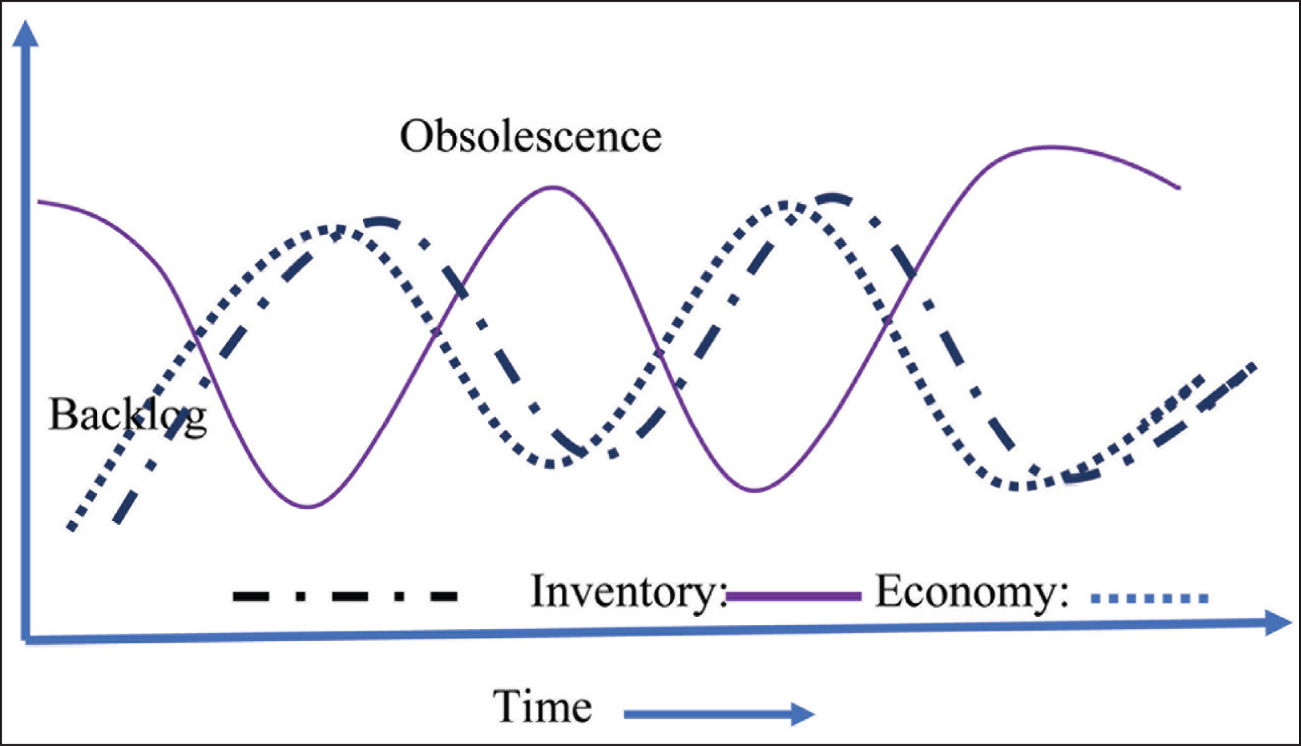
Figure 12 shows that as the economy slows down, inventory goes up, leading to obsolescence; on the other hand, as the economy recovers, inventory is expected to come down and backlog will increase unless the production gets ramped up. However, ramping up will depend on producers’ confidence to invest further or use additional resources and availability of inputs to production. The availability of inputs to production will depend on suppliers’ capability and willingness to ramp up their productions and logistics, ensuring the flow of goods.

The Proposed Model

The proposed model suggests that the rate of change of production (Qt) is dependent on the difference between the inventory and backlog and the number or quantity of order received, as shown in Equation 1.

d Q_{t d} = [\partial O_{t} - (I_{t} - B_{t})] * L

(1)

Where dQ_td is the desired rate of production in time t

O_t is the rate of order in time

I_t is the inventory in time t

B_t is the backlog in time t

L is the logistics factor affecting the shipment of inbound goods.

Equation 2 shows that the order rate is the product of a change in demand D_t for the specific goods and the market share or preference of the product (C) denoted as M_t at the given point of time t.

\partial O_{t} = D_{t} * M_{t}

(2)

Where ∂O_t is the order rate

D_t is the demand at time t

Demand D_t is dependent on the change in income or price and the corresponding elasticities for the given product C.

Equation 3 shows the relationship between change in demand D_t,P,_INdue to price and income elasticity e_p, and e_i respectively of goods C.

D_{t, P, I N} = D_{0} * P^{e_{p}} * I N^{e_{i}}

(3)

Where P represents the price of goods

Where IN represents the income of consumers

Income (IN_t) at a time is disrupted due to pandemic, that is, the force majeure factor (f_f) as shown in Equation 4.

I N_{t} = I N_{t - 1} * f f

(4)

f_f takes a value between 0 and 1, where 0 signifies complete stoppage of business while 1 denotes regular activity.

The force majeure factor (f_f),also impacts the logistics. Equation 5 shows the relationship between the state-of-logistics (L_t) and the force majeure factor (f_f).

L_{t} = L_{t 1} * f_{f}

(5)

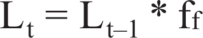
Equation 1 shows the production quantity at a time provided the flow of inputs is uninterrupted. However, the supply is affected during force majeure conditions; hence, Equation 1 is re-written as:

d Q_{t a} = [\partial O_{t} - (I_{t} - B_{t})] * L_{t}

(6)

The disruption in production causes backlog to increase. Thus, Equation 8 shows the increase in backlog as the actual production drops below the desired level.

[(B_{t})] = [\partial O_{t} - I_{t}] - \frac{d Q_{t a}}{L_{t}}

(7)

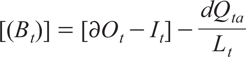
where dQ_ta is the actual rate of production.

The desired rate of production is $d Q_{t d} = \frac{d Q_{t a}}{L_{t}}$ . This disruption causes a supply shock and along with disruption in the logistics system, the cost of logistics increases leading to an increase in the price of finished goods. The increase in price, in turn, reduces the demand for normal-goods. This circular causality is required to be inbuilt in the model.

Equation 8 suggests the supply-price relationship.

P_{t} = P_{t - 1} * [1 + r]

(8)

Here, r is the rate of increase due to logistics supply shock.

Recently, the leading Indian car manufacturer declared an increase in its price to the extent of 5 per cent (ToI, 2020) and in April 2020, transporters announced an 80 per cent increase in the cost of logistics (ET, 2020). A study shows that machinery transportation is around 18 per cent in India (Pratap et al., 2020).

Thus, the model needs to update the changes in supply and demand conditions as one factor counter influences the other. An SD model based on the above framework can capture the direct and circular causalities. This SD model can enable a decision-maker to simulate the situations under different economic and supply conditions. The next section describes the SD model.

The System Dynamics (SD) Model

Forrester (1961, 1997) laid down the foundation of SD called industrial dynamics. This approach captures the way organisational structure, policies and time delays (in decisions and actions) influence organisations’ success. It allows interactions between the flow of resources, information, and external shocks, like economy, to study their impact on the outcomes, such as sales, revenue, inventory or backlogs. Senge (1990) extended SD to systems thinking, that is, contemplating the whole, and termed it as the fifth discipline to ensure organisational success. He substantiated the interrelatedness between the factors that may subtly give rise to effects but make the dynamics complex. That is, the short and long term effects are significantly different. In this research, the authors simulate such effects varying the impact of the pandemic (referred to as force majeure) on the exogenous factors such as income and price and endogenous ones, namely the rates of production and supply. The proposed model captures the interconnectedness and sees the impact on supply chain drivers such as inventory (Chopra & Meindl, 2001). There are several instances of SD indicating its application in the study of supply chain management (Angerhofer & Angelides, 2000). The most significant utility of an SD approach is its ability to include non-linearity and circular causality in the models (Forrester, 1994).

Figure 13 illustrated the system dynamics (SD) model developed in line with the proposed model described in the previous section.

Figure 13.

Source: Authors’ creation using Vensim software.

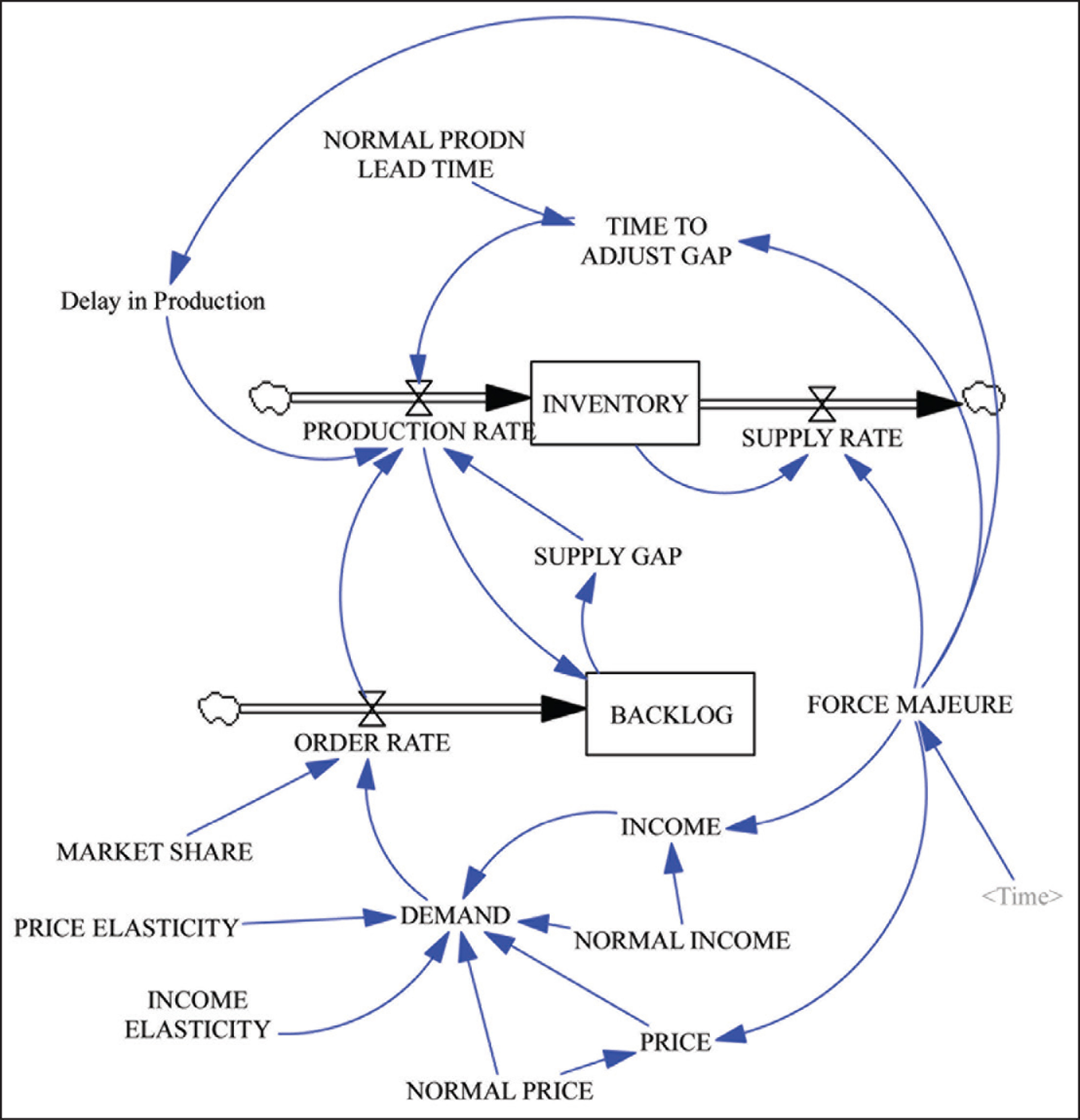
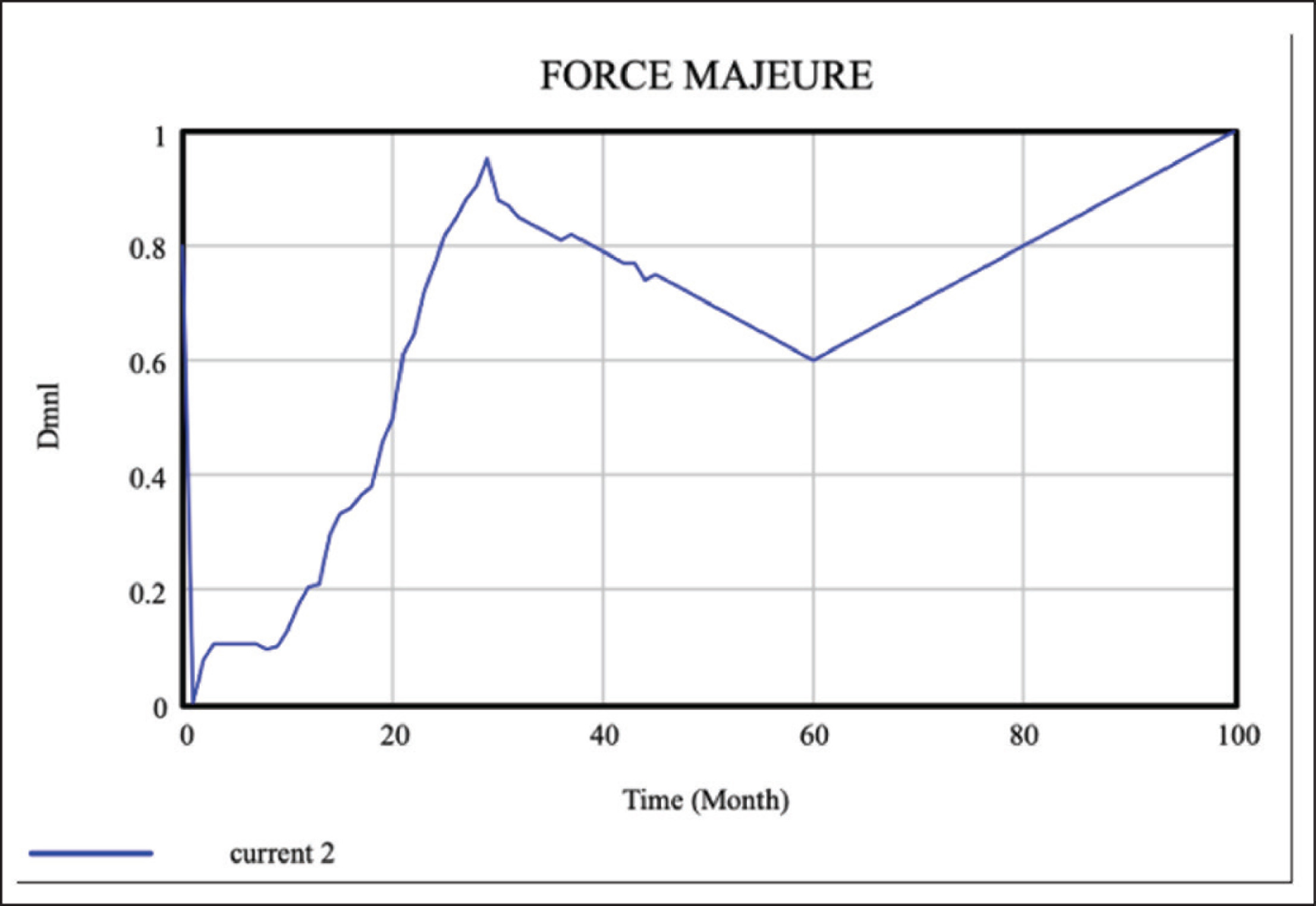
The model shows the pandemic’s (referred to as force majeure in the SD model) influence on the state of the business. The peculiarity of the model is in its ability to capture the supply and the demand shocks simultaneously. The force majeure impacts the income as businesses halts and prices as the supply chain gets disrupted. This factor is treated as a trend to capture its impact instead of a constant. Experts now opine it is uncertain to recommend time to return to normalcy. Hence, the model is simulated for 100 months, that is, approximately four years. Figure 14 demonstrates the impact indicating that it may appear to normalcy in two years, but due to the return of the second wave of the disease or so, the business may drop to say a 60 per cent level. Then, on the stability of medicines, vaccines, working protocols and treatment efficiencies, the situation bounces to normal unless some other disruption occurs. This depiction is the authors’ assumptions and any researcher can simulate the model with different trends.

Figure 14.

Source: Authors.

The variables (rate, level, auxiliary and constant) used in this model include:

Level variables:

B_t = The backlog in time

_t = The inventory in time t

Rate variables:

∂O_t = The rate of order in time t

∂Q_t = The rate of production in time t

∂S_t = The rate of supply in time t

∂Q_m = Maximum production rate in time t

Auxiliary variables:

D_t,P,I = Demand in time t, when price of product is P and income of buyers is I

P_t = Current price, i.e., during post – COVID period, say, June, 2020

IN_t = Current income, i.e., during post – COVID period, say, June 2020

M_t = Market share in time t

S_g = Supply gap

T_g = Time to adjust gap

D_e = Delay in production due to force majeure factor

Constants:

I_vb = Initial value of backlog

I_vi = Initial value of inventory

D₀ = Demand during pre – COVID period, say, December, 2019

P₀ = Normal price, i.e., during pre – COVID period, say, December, 2019

IN₀ = Normal income, i.e., during pre – COVID period, say, December 2019

e_p = Price elasticity

e_i = Income elasticity

L_n =Normal production lead time

T = Per unit time for simulation, equal to one month in this model.

Table graph values:

f_f = Force majeure factor, is a lookup table—a time–factor graph

The equations used in the model include:

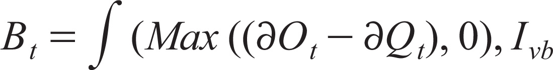
B_{t} = \int^{​} (\max ((\partial O_{t} - \partial Q_{t}), 0) I_{v b}

(9)

Equation 9 indicates the computation of backlog, which is the difference between the order rate and the production rate, with an initial value of backlog before the start of the simulation.

\begin{matrix} D_{t, P, I N} = I f T h e n E l s e ​ (I N_{t} \leq ​ 6000, 0.01, (D_{0} * ((P_{0} \div P_{t})^e_{p}) \\ * ((I N_{t} \div I N_{o})^e_{i}))) \end{matrix}

(10)

Equation 10 indicates that the demand is the function of initial demand and change in price and income and their elasticities. The demand is negligible (say, 0.01) when income drops below a certain level, say, $6000.

I N_{t} = f_{f} * I N_{o}

(11)

Equation 11 indicates that the current income is a function of normal-income and the force majeure factor.

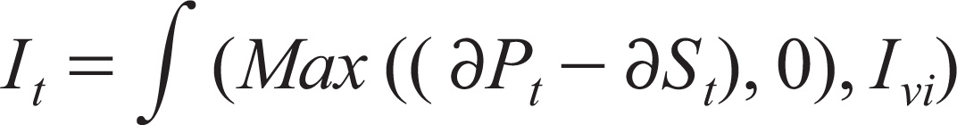
I_{t} = \int^{​} (\max ((\partial P_{t} - \partial S_{t}), 0) I_{v i})

(12)

Equation 12 indicates that the inventory is the difference between the production and supply rate with the initial inventory before the simulation run.

\partial O_{t} = D_{t, P, I N} * M_{t}

(13)

Equation 13 indicates that the order rate is the function of demand for the firm’s goods and market share.

P_{t} = \max ((P_{o} * (1 \div f_{f})), P_{o})

(14)

Equation 14 indicates that the price is a function of normal-price and the force majeure subject to the condition that the same does not drop below the normal-price.

\partial Q_{t} = (\min (((\partial O_{t} \div D_{e}) + (S_{g} \div T_{g})), \partial Q_{m}))

(15)

Equation 15 indicates that the production rate is the sum of the order rate and the supply gap in the previous month subject to the condition that the production rate has a specified maximum level. Every organisation has a limitation in increasing the production rate.

S_{g} = \max (B_{t}, 0)

(16)

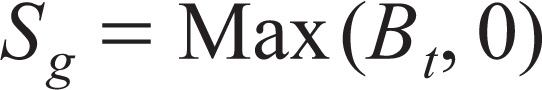
Equation 16 indicates that the supply gap is the backlog and does not take negative values.

\partial S_{t} = A c t i v e I n i t i a l (((I_{t}) * f_{f}), 10)

(17)

Equation 17 indicates that the supply rate is the function of the inventory and the force majeure factor. The initial rate of supply has been taken as 10 per month.

T_{g} = (1 \div f_{t}) * L_{n}

(18)

Equation 18 shows that a firm needs time to adjust its production rate beyond normal. As there is a backlog that requires ramp-up of production, the minimum time to do this is the ‘Time to Adjust Gap’. In times of pandemic, the standard production time is affected by the force majeure factor.

D_{e} = (1 \div f_{t}) * T

(19)

Equation 19 defines the delay in production as a function of force majeure factor, and per-unit time considered for simulation. In this model, the per unit time is taken as per month. That is, all rates, demand and income are values per month.

The model was validated using the case of a normal good. The simulation set up includes a timeline of 100 months and assumes that if the normal-monthly income (considered as 10,000 monetary units, say USD) drops below a certain amount ($6000), there is no demand for any normal or price elastic goods. The authors provide the initial values of level and auxiliary variables and constants such as price and income elasticities.

Figure 15 shows the model’s output compared to the baseline, that is, if there is no pandemic. The baseline structure serves as the reference model.

Figure 15.

Source: Authors.

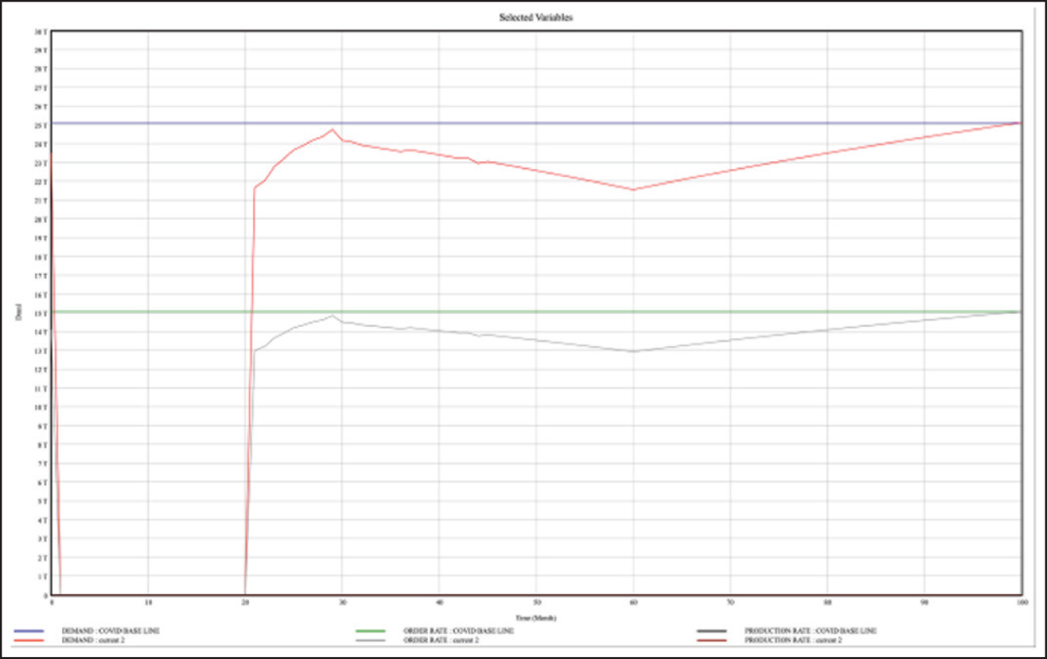
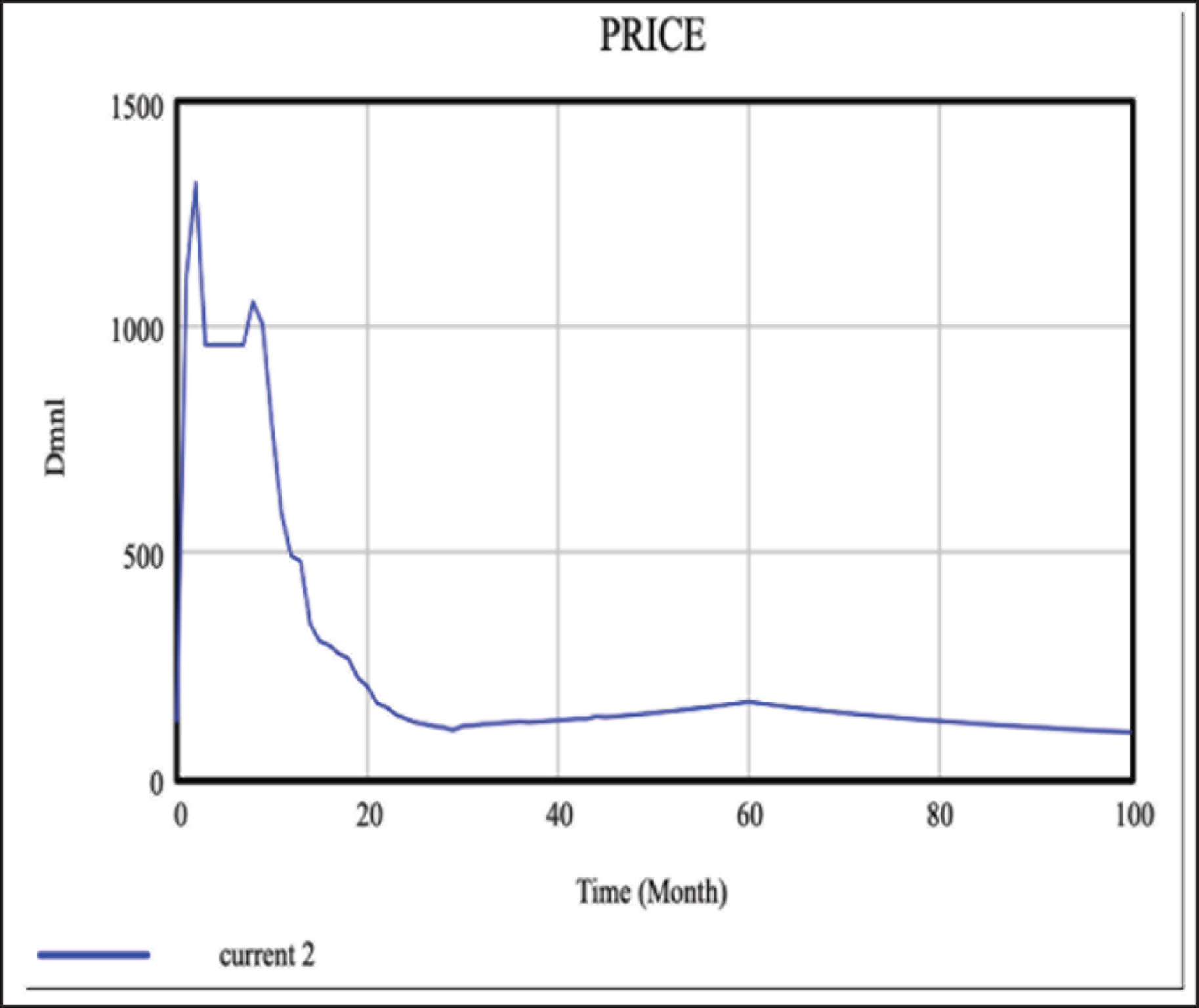
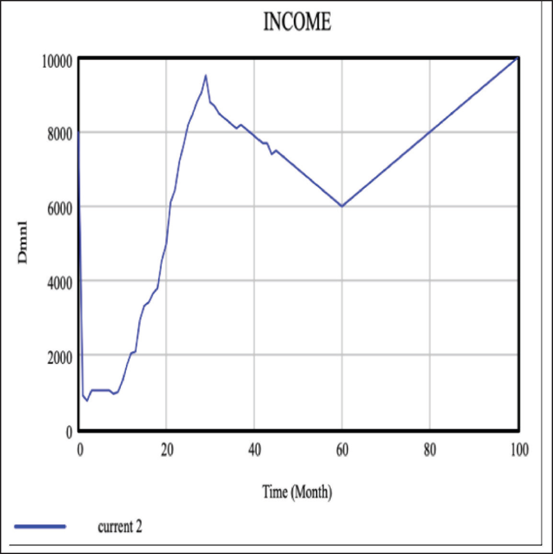
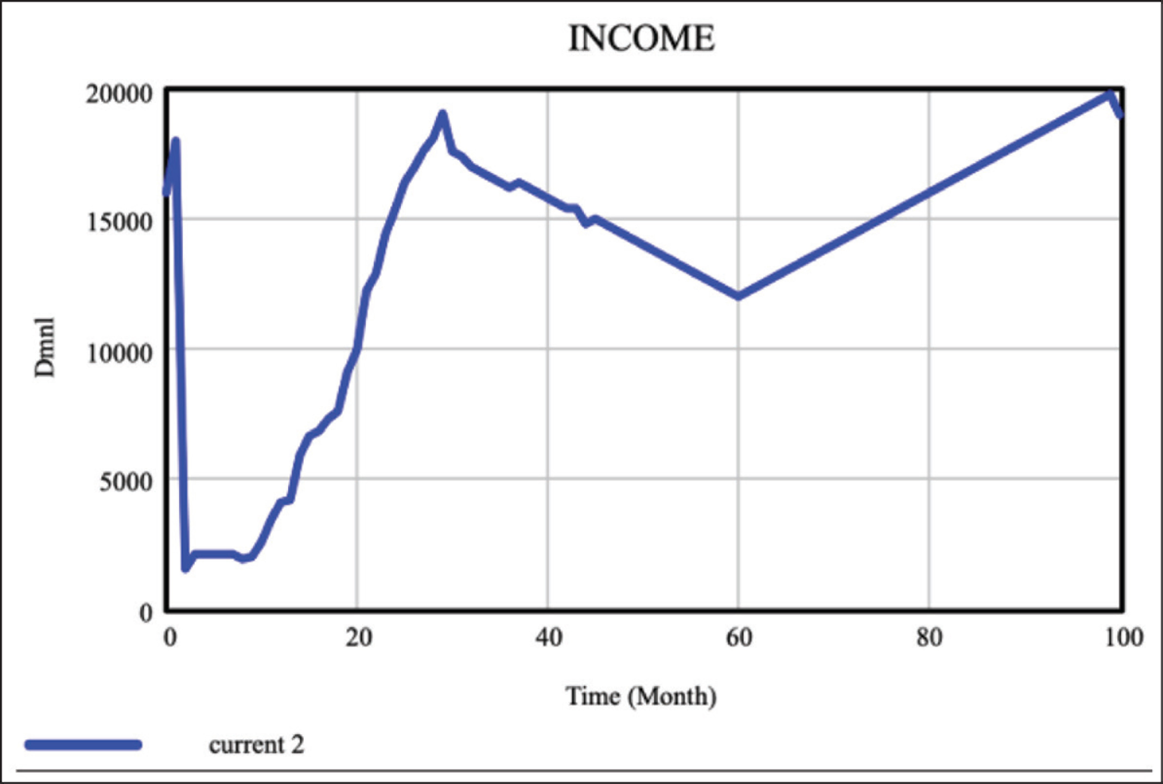
Figures 16 and 17 demonstrate the price and income scenario post-pandemic. The graphs have similar trends indicating that during the lockdown period, the prices go up and income reduces.

Figure 16.

Source: Authors’ Vensim Model.

Figure 17.

Source: Authors’ Vensim Model.

The production-rate varies with order rate and backlog, as it is the sum of the order placed and previous backlog.

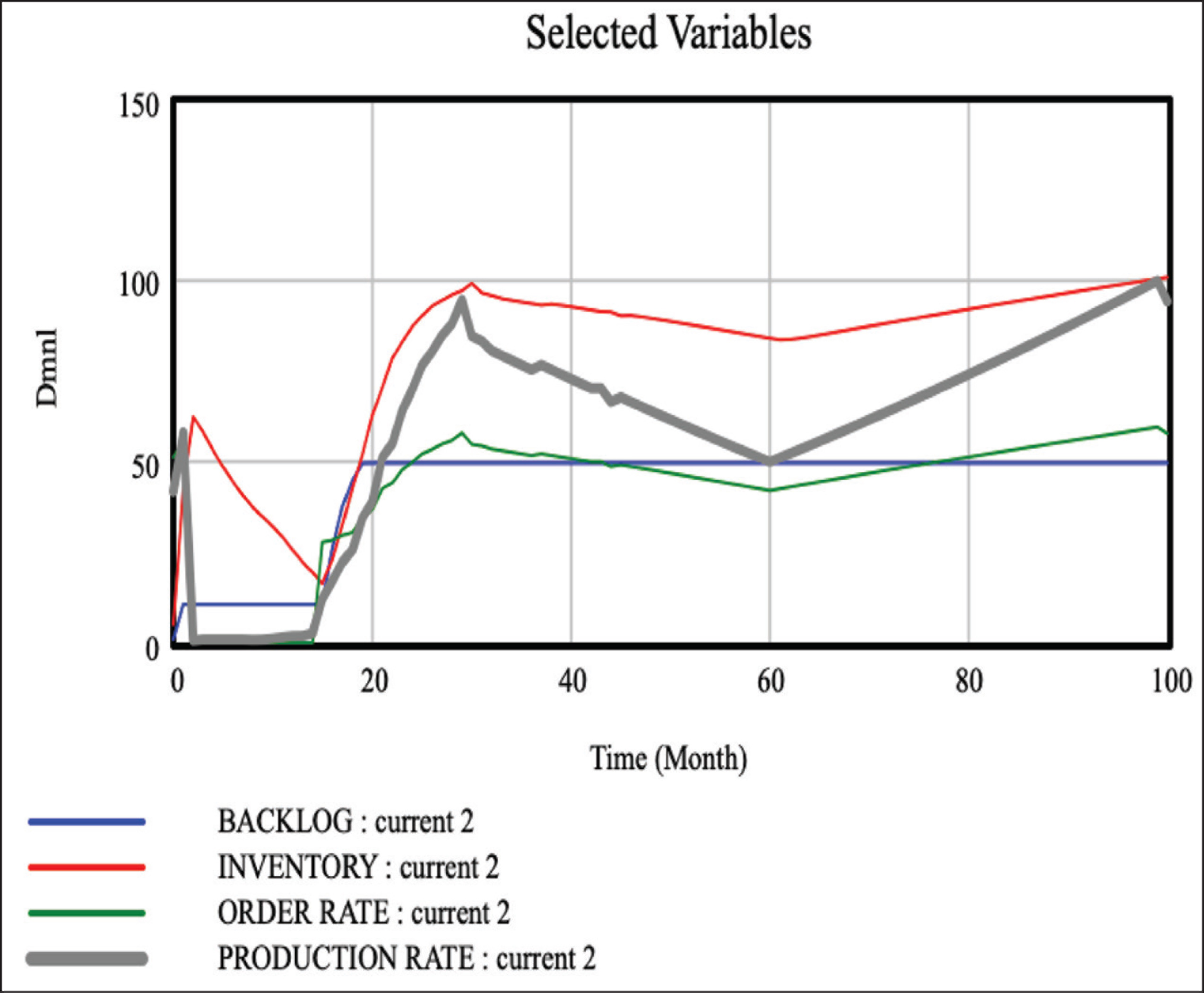
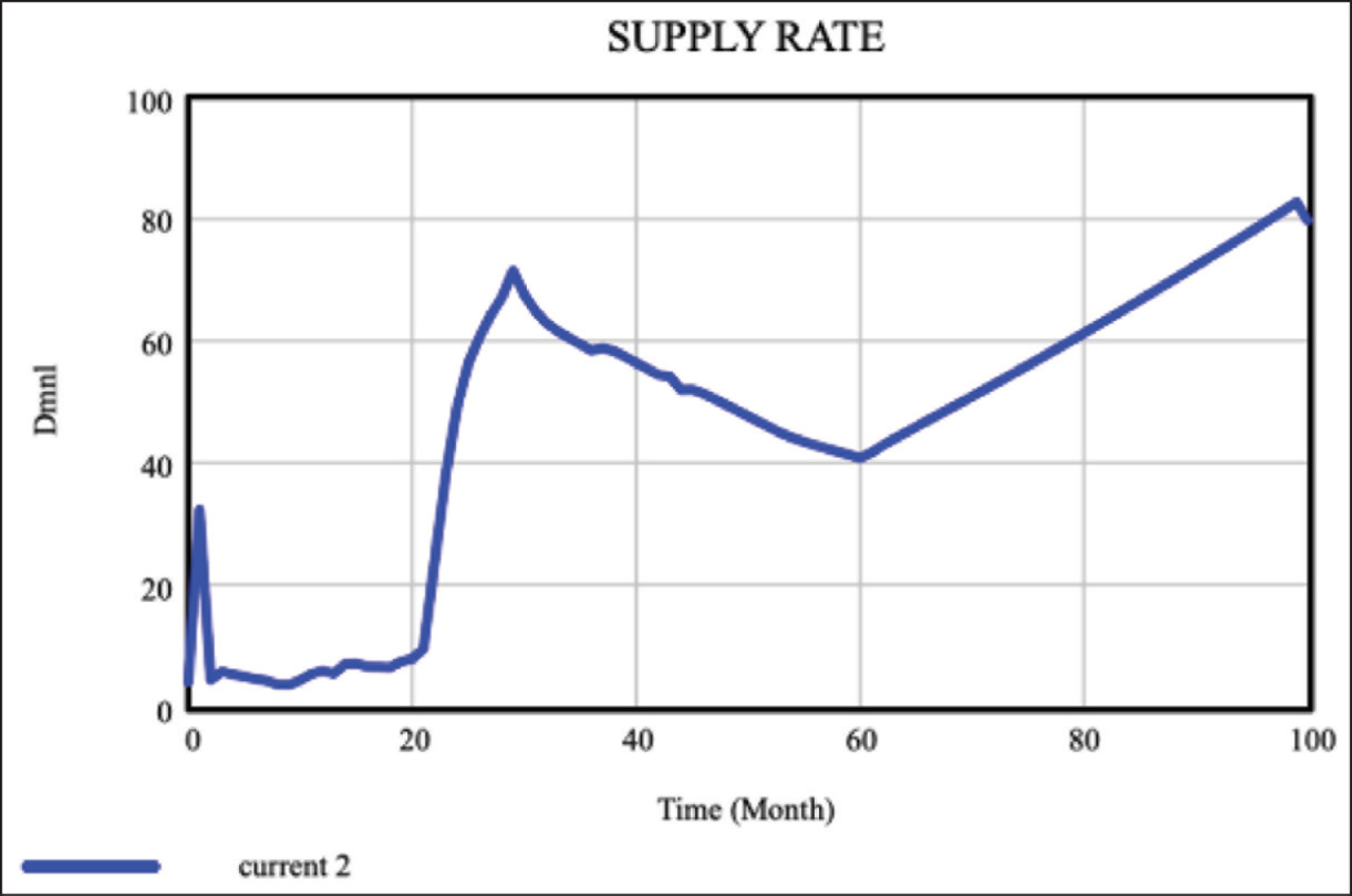
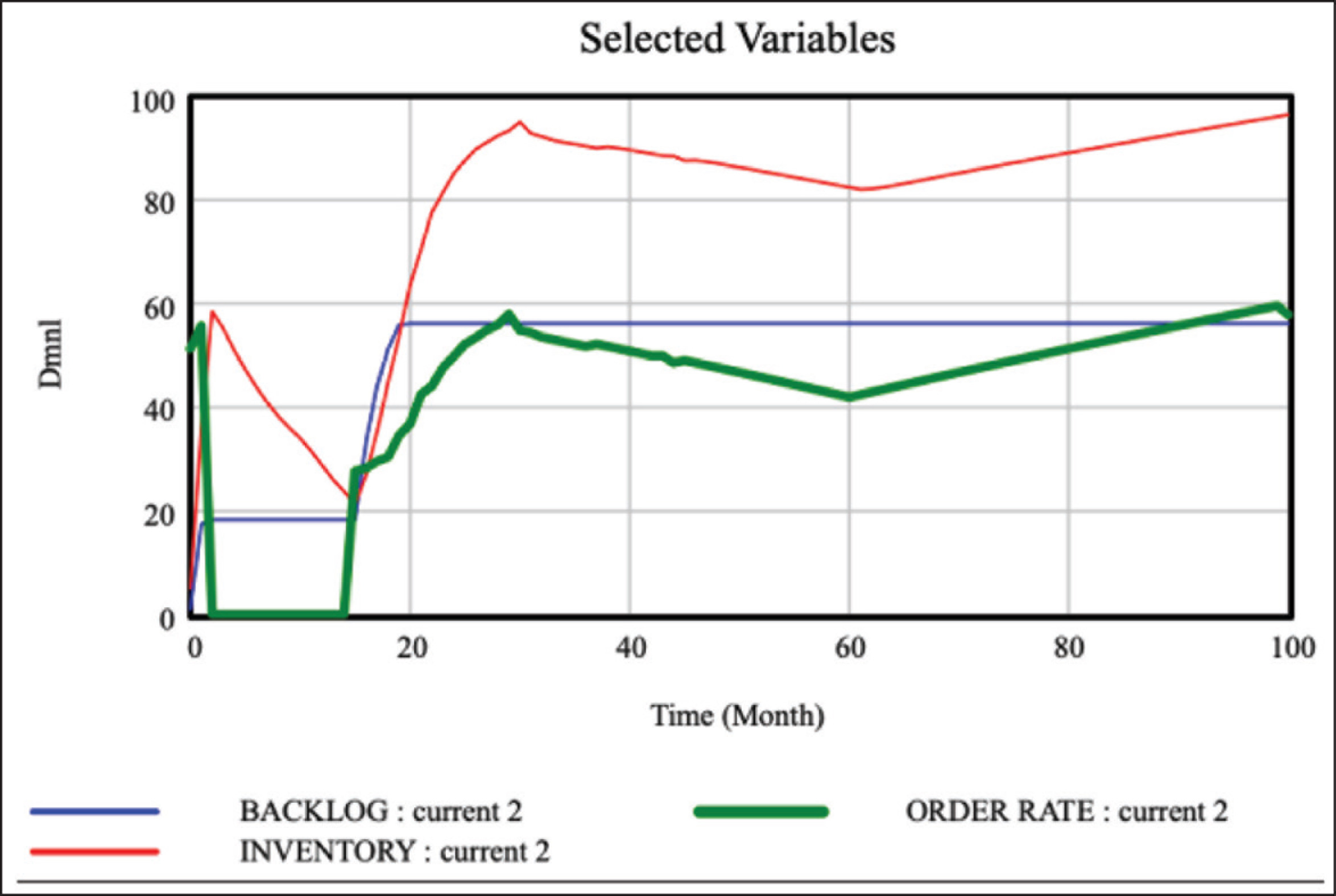
Figures 18 and 19 show that the backlog stabilises in the long run, but the inventory and production rate exhibit variance in line with the force majeure impact (shown in Figure 14), that is, it increases as the economy recovers. The variance in supply rate is shown in Figure 20, indicating that as the force majeure factor causes business to halt the supply rate drops and increases as the situation recovers. If the normal-income increase (say due to incentives by the government), say by two times, the maximum backlog and inventory levels also increase by 1.5 and 1.12 times, respectively. The increase in income causes the order rate to go up, but the backlog and inventory levels increase as the production rate, and supply remains unchanged. Hence, inbound and outbound flows need to be restored for the economy to grow. Figures 21 and 22 demonstrate the impact of an increase in income and corresponding levels of backlog and inventory.

Figure 18.

Source: Authors’ creation—simulation results using Vensim software.

Figure 19.

Source: Authors’ creation—simulation results using Vensim software.

Figure 20.

Source: Authors’ creation—Simulation results using Vensim software.

Figure 21.

Source: Authors’ creation— Simulation results using VENSIM software.

Figure 22.

Source: Authors’ creation— Simulation results using VENSIM software.

Thus, the model captures the proposed trend, as described in Figure 9.

Conclusion

The authors presented the difference in pre- and post-pandemic environments. The article suggests that unlike usual supply chain strategy to comprehend for alternate supply sources and/or markets does not hold good in the COVID-19 like situations as the whole world is affected by the pandemic. The supply of inputs, production rates and the flow of finished goods are all impacted simultaneously. It also means that the businesses are stalled or slowed down and thus the income and consumptions take a toll. The impact on demand for goods varies with their corresponding elasticities (income and price). This article identifies the relationship between the economic and operational factors and uses them to develop a SD model. The SD model simulation can aid policy experimentation, such as the impact of demand- and supply-side incentives (by the government) and operational strategy on return to normalcy. The results show that the flow of goods (inputs and finished goods) are crucial in salvaging the situation. Even though income increases the orders, but slower rates of supplies nullify the effect.

This model can be extended to capture any country’s scenario, any product under different lockdown scenarios. As further research, the econometric relationships at the country, firm and product level can be assessed, validated and simulated for policy and strategy experimentation. The future study may include the impact of green factors on supply chain disruptions as one of the probable cause of the COVID-19 virus is the unhygienic method of slaughtering animals in the wet-market in Wuhan, China.

Footnotes

Declaration of Conflicting Interests

The authors declared no potential conflicts of interest with respect to the research, authorship and/or publication of this article.

Funding

The authors received no financial support for the research, authorship and/or publication of this article.

References

Angerhofer

B. J.

, & Angelides

M. C.

(December 2000). System dynamics modelling in supply chain management: Research review. In 2000 Winter Simulation Conference Proceedings (Cat. No. 00CH37165), Vol. 1, pp.342–351. IEEE.

Bloomberg (2020). https://www.bloomberg.com/amp/news/articles/2020-04-06/ship-crews-stuck-in-lockdown-strain-global-supply-chains

Bowersox

D. J.

, Closs

D. J.

, & Hall

C. T.

(1998). Beyond, E.R.P.—the storm before the calm. Supply Chain Management Review, 1(4), 28–37.

Cabral

, Grilo

, & Cruz-Machado

(2012). A decision-making model for lean, agile, resilient and green supply chain management. International Journal of Production Research, 50(17), 4830–4845.

Carvalho

, Duarte

, & Machado

V. C.

(2011). Lean, agile, resilient and green: Divergencies and synergies. International Journal of Lean Six Sigma, 2(2), 151–179.

Carvalho

, & Machado

V.C.

(2009). Lean, agile, resilient and green supply chain: A review. Proceedings of the 3rd international conference on management science and engineering management, 2–4 November, Bangkok, Thailand. World Academic Press, World Academic Union, pp. 66–76.

Chopra

, & Meindl

(2001). Supply chain management: Strategy, planning, and operation. Prentice Hall.

Christopher

(1998). Logistics and supply chain management: Strategies for reducing costs and improving services. Pitman Publishing.

Christopher

, & Towill

(2000). Supply chain migration from lean to agile and customised. Supply Chain Management, 5(4), 206–213.

10.

Cox

, Sanderson

, & Watson

(2000). Power regimes mapping the DNA of business and supply chain relationships. Earlsgate Press.

11.

Dahl

C. A.

(1995). Demand for transportation fuels: A survey of demand elasticities and their components. The Journal of Energy Literature, 1(2), 3–27.

12.

Dargay

, & Gately

(1997). Vehicle ownership to 2015: Implications for energy use and emissions. Energy Policy, 25(14–15), 1121–1127.

13.

Deloitte (2020). Kalish, Ira. https://www2.deloitte.com/us/en/insights/economy/global-economic-outlook/weekly-update.html, (accessed on 24 June 2020 ).

14.

Espey

(1998). Gasoline demand revisited: An international meta-analysis to elasticities. Energy Economics, 20(3), 273–295.

15.

Economic Times [ET]. (2020). https://economictimes.indiatimes.com/industry/transportation/shipping-/-transport/logistics-costs-set-to-rise-as-freighters-hike-tariffs/articleshow/75129422.cms?utm_source=contentofinterest&utm_medium=text&utm_campaign=cppst (accessed on 24 June 2020 ).

16.

Fine

C. H.

(1998). Clockspeed: Winning industry control in the age of temporary advantage. Perseus Books.

17.

Forrester

J. W.

(1994). System dynamics, systems thinking, and soft OR. System dynamics review, 10(2–3), 245–256.

18.

Forrester

J. W.

(1997). Industrial dynamics. Journal of the Operational Research Society, 48(10), 1037–1041.

19.

Goldman

S. L.

, Nagel

R. N.

, & Preiss

(1995). Agile competition and virtual organisations, Van Nostrand Reinhold.

20.

Goodwin

, Dargay

, & Hanly

(2004). Elasticities of road traffic and fuel consumption with respect to price and income: A review. Transport Reviews 24(3), 275–292.

21.

Greenman

J. V.

(1996). The car park: Diffusion models revisited. Energy Economics, 18(1–2), 107–128.

22.

Harland

C. M.

, Lamming

R. C.

, & Cousins

P. D.

(1999). Developing the concept of supply strategy. International Journal of Operations & Production Management, 19(7), 650–673.

23.

Harrison

, Christopher

, & van Hoek

(1999). Creating the agile supply chain (Working paper). School of Management, Cranfield University, Cranfield.

24.

Hoek

R. V.

, Harrison

, & Christopher

(2001). Measuring agile capabilities in the supply chain. International Journal of Operations & Production Management, 21(1–2), 126–148.

25.

Huang

G. Q.

(1996). Design for X: Concurrent engineering imperatives. Chapman and Hall.

26.

Ismail

H. S.

, & Sharifi

(2006). A balanced approach to building agile supply chains. International Journal of Physical Distribution & Logistics Management, 36(6), 431–444.

27.

Ismail

H. S.

, Snowden

, Toward

, Christian

, Mooney

, & Zhang

(2001). Agile manufacturing transitional strategies. Paper presented at 4th SMESME International Conference, Aalborg, pp. 69–77.

28.

JICA (Japan International Cooperation Agency) 2013. What are major important lessons learned from past disasters, including the Great East Japan Earthquake? [Online]. http://siteresources.worldbank.org/JAPANINJAPANESEEXT/Resources/515497-1196389582361/4451844-1331081087023/Fuwa.pdf

29.

Kehoe

D. F.

, Sharifi

, Boughton

N. J.

, Burns

N. D.

, & Dani

(2006). Demand network alignment: Aligning the physical informational and relationship issues in a supply chain. International Journal of Production Research (print).

30.

Koshimura

, & Shuto

(2015). Response to the 2011 great East Japan earthquake and tsunami disaster. Philosophical Transactions of the Royal Society A: Mathematical, Physical and Engineering Sciences, 373(2053), 20140373.

31.

Lescaroux

, & Rech

(2008). The impact of automobile diffusion on the income elasticity of motor fuel demand. The Energy Journal, 29(1), 41–60.

32.

Marley

K. A.

(2006). Mitigating supply chain disruptions: Essays on lean management, interactive complexity, and tight coupling. Doctoral Dissertation, The Ohio State University.

33.

McRae

(1994). Gasoline demand in developing Asian countries. The Energy Journal, 15(1), 143–155.

34.

Medlock

K. B.

, & Soligo

(2002). Car ownership and economic development with forecasts to the year 2015. Journal of Transport Economics and Policy, 36(2), 163–188.

35.

Moynihan

2009. The response to Hurricane Katrina [Online]. https://irgc.org/wp-content/uploads/2018/09/Hurricane_Katrina_full_case_study_web.pdf

36.

Nagel

, & Dove

(1991). 21st Century Manufacturing Enterprise Strategy – An Industry Led Review (Vols 1 and 2). Bethlehem, PA: Iacocca Institute, Lehigh University.

37.

Neto

(2012). Testing and estimating time-varying elasticities of Swiss gasoline demand. Energy Economics, 34(6), 1755–1762.

38.

Ohio State University 2013. Resilience and Sustainability [Online]. http://resilience.osu.edu/CFR-site/resilienceandsustainability.htm

39.

Pratap

, Gupta

D. B.

, & Pohit

(2020). Quantifying macro logistics cost of India. NCAER. http://www.ncaer.org/publication_details.php?pID=325, (accessed on 08.06.2020).

40.

Schmidt

, & Raman

2012. When supply-chain disruptions matter [Online]. Harvard Business School. http://www.hbs.edu/faculty/Publication%20Files/13-00

41.

Senge

P. M.

(1990). The art and practice of the learning organization. https://doi.org/10.1002/hrm.3930290308

42.

Shakir Ullah

, Huaccho Huatuco

, & Burgess

T. F.

(2016). A literature review of disruption and sustainability in supply chains. InImpact: The Journal of Innovation Impact, 7(2), 500.

43.

Sharifi

, & Zhang

(1999). A methodology for achieving agility in manufacturing organizations: An introduction. International Journal of Production Economics, 62(1/2), 7–22.

44.

Sharifi

, Ismail

H. S.

, & Reid

(2006). Achieving agility in supply chain through simultaneous “design of” and “design for” supply chain. Journal of Manufacturing Technology Management, 17(8), 1078–1098. https://doi.org/10.1108/17410380610707393

45.

Sinha

, & Dey

(2018). Supply chain strategies to sustain economic and customer uncertainties. In Dhir

& Shishil

(Eds.), Flexible strategies in VUCA markets (pp. 139–153). Springer.

46.

Times of India [TOI]. (2020). https://timesofindia.indiatimes.com/business/india-business/maruti-hikes-select-model-prices-by-up-to-rs-10000/articleshow/73669955.cms (accessed on 24 June 2020 ).

47.

United Nations [UN] (2012). Disaster risk and resilience [Online]. https://www.un.org/development/desa/dpad/publication/world-economic-situation-and-prospects-april-2020-briefing-no-136/; accessed on 08.06.2020

48.

United Nations [UN] (2020). https://www.un.org/development/desa/dpad/publication/world-economic-situation-and-prospects-april-2020-briefing-no-136/. (Accessed on 08.06.2020).

49.

Van der Vorst

J. G. A. J.

, & Beulens

A. J. M.

, 2002. Identifying sources of uncertainty to generate supply chain redesign strategies. International Journal of Physical Distribution & Logistics Management, 32(6), 409–430.

50.

Web Desk (2020). https://www.theweek.in/news/world/2020/04/21/explainer-oil-prices-negative-us-wti-what-does-it-mean-consumers-pump-gas-prices.html#:~:text=Demand%20for%20oil%20has%20collapsed,storing%20crude%20are%20nearly%20full.&text=In%20summary%2C%20the%20steep%20fall,to%20address%20the%20supply%20glut (accessed on 08 June .2020)

51.

Wilkie

D. S.

, & Godoy

R. A.

(2001). Income and price elasticities of bushmeat demand in lowland Amerindian societies. Conservation Biology, 15, 761–769.

The Supply Chain Disruption Framework Post COVID-19: A System Dynamics Model

Abstract

Keywords

Introduction

The Existing Model

The Current Situation

Supply Chain Strategies: A Literature Review

The Conceptual Model

The Proposed Model

The System Dynamics (SD) Model

Conclusion

Footnotes

Declaration of Conflicting Interests

Funding

References