Cumulant-Based Approaches for Testing the Assumption of Independent Errors in Non-Gaussian Parallel and Congeneric Measures

Abstract

In classical test theory, independence of measurement errors constitutes a central assumption when estimating the reliability of measures. Furthermore, it is well known that this assumption cannot be tested with standard methods that rely on second-order moments (variances, covariances). The present study, therefore, explores properties of non-Gaussian parallel and congeneric measures (i.e., when observed scores deviate from the Gaussian distribution) with respect to their capabilities of identifying violations of the error independence assumption. We show that, under non-Gaussianity and inequality of hidden confounding effects, third and fourth cumulant-based test statistics can be derived which enable researchers to detect non-independent error structures. We describe identifiability conditions under which the proposed test statistics can be expected to have adequate statistical power in parallel and congeneric measures and present results of Monte-Carlo simulation experiments. Results suggest that third-order tests adequately protect the nominal significance level. However, fourth-order tests can produce inflated Type I error rates, in particular, when error variances are unequal. In general, the power to detect non-independent errors increases with the sample size, the magnitude of non-Gaussianity, the degree of inequality of hidden confounding effects, and the degree of error non-independence. A real-world data example is presented for illustrative purposes. The current study presents important insights for developing statistical methods to detect error non-independence. However, these methods also rest on crucial assumptions, emphasizing the severity of the issue of statistically detecting non-independent measurement errors.

Introduction

The Classical Test Theory (CTT) framework (e.g., Lord & Novick, 1968; Zimmerman, 1975) defines an observed score (X) as the sum of a true score (T) and an error score (E), that is, X = T+E. The true score is defined as T = $\mathbb{E}[X|\sigma (f)]$ where $\mathbb{E}$ denotes the expected value operator, f represents the assignment-to-individual function, and $\sigma (f)$ is the set of measurable events generated by f (Kroc & Zumbo, 2020; Zimmerman & Zumbo, 2001). In other words, each individual receives one true score that remains fixed under (active or hypothetical) repeated measurements. Two consequences emerge from this true score definition: (a) the expected value of the measurement error is zero, that is, $\mathbb{E}[E|\mathrm{\sigma }\left(f\right)]=\mathbb{E}[X|\mathrm{\sigma }\left(f\right)]-\mathbb{E}[T|\mathrm{\sigma }\left(f\right)]=T-T$ = 0 and (b) true scores and errors are uncorrelated, that is, cov(T, E) = $\mathbb{E}$ [TE] = $\mathbb{E}\left\{T\mathbb{E}[E|\mathrm{\sigma }\left(f\right)]\right\}$ = 0 (Kroc & Zumbo, 2020; Zumbo, 2025).

The present article focuses on pairs of measures. Let X₁ = T₁+E₁ and X₂ = T₂+E₂ be observed test scores with T₁ and T₂ denoting the true scores and E₁ and E₂ representing the corresponding errors. For measures to be parallel, we assume that T = T₁ = T₂ (i.e., each measure is based on a common true score) and var(E₁) = var(E₂) = ${\sigma }_E^2$ implying that the two error components have the same variance ${\sigma }_E^2$ . In other words, for measurements being parallel, it is assumed that two tests measure the same latent true score (T) with equal measurement precision ( ${\sigma }_E^2$ ). In contrast, measurements are τ-equivalent when tests measure the same latent true score (T) with possibly different error variances, that is, ${\sigma }_{E_1}^2\ne {\sigma }_{E_2}^2$ . Formally, parallel (and τ-equivalent) models can be expressed as

$$X_1=T+E_1\mathrm{and}{X}_2=T+E_2.$$

(1)

In addition, in any psychometric application, one assumes that the error terms E₁ and E₂ are uncorrelated, that is, cor(E₁, E₂) = 0, which is referred to assuming “linear experimental independence” (Zimmerman & Williams, 1980). The reason for this is that, even when the parallel measures have the same variance (var(X₁) = var(X₂) = ${\sigma }_X^2$ ) and the same reliability $\rho$ (i.e., the ratio of true and observed score variance or, alternatively, one minus the ratio of the error variance and the observed score variance ¹ ), the correlation between the two measures no longer corresponds to the reliability of either measure (e.g., Raykov et al., 2015; Zimmerman & Williams, 1980), that is,

$$\mathrm{cor}(X_1,X_2)=\rho +\mathrm{cor}(E_1,E_2)(1-\rho ).$$

(2)

From Equation 2 it follows that $\mathrm{cor}(X_1,X_2)=\rho$ holds only if $\mathrm{cor}(E_1,E_2)$ = 0. In contrast, when $\mathrm{cor}(E_1,E_2)\ne$ 0, the discrepancy between $\mathrm{cor}(X_1,X_2)$ and $\rho$ depends directly on the correlation between errors and inversely on the reliability. That is, $\mathrm{cor}(X_1,X_2)$ exceeds $\rho$ when $\mathrm{cor}(E_1,E_2)$ > 0, and $\rho$ exceeds $\mathrm{cor}(X_1,X_2)$ when $\mathrm{cor}(E_1,E_2)$ < 0.

Several decades ago, various researchers articulated concerns about the plausibility of the assumption of independent errors (see, for example, Cronbach, 1947; Guttman, 1953; Williams, 1974) and various examples exist in which this assumption is unlikely to be fulfilled, such as changes in the examinee’s motivation, test fatigue, or presenting parallel tests closely in time or space (see, for example, Cocker & Algina, 2006; Furlan & Sterr, 2018; Sörbom, 1975; Wyse, 2021). Furthermore, it is well known that the independent errors assumption cannot be empirically tested using standard covariance-based analysis. For example, Raykov et al. (2015) showed that the covariance matrix of a parallel test model (i.e., two measures with the same loadings on a common true score, equal measurement precision, and uncorrelated errors) is identical to the covariance matrix of a relaxed parallel test model which does not assume uncorrelated errors.

Arguably, the detection of correlated measurement errors in two measures constitutes a long-standing, yet unsolved psychometric problem. In addition, any methodological approach that allows researchers to critically evaluate the assumption of independent errors in pairs of measures can also be expected to be valuable for settings in which latent traits are estimated using more than two measurement indicators. In confirmatory factor-analytic settings, for example, the issue of correlated errors is well known. Here, researchers usually address the issue of correlated errors through allowing residual correlations in the factor model. However, this research practice is not free of criticism (Gerbing & Anderson, 1984; Landis et al., 2009; Tomarken & Waller, 2003). Although design-driven inclusion of correlated residuals is, in some cases, recommended to avoid biased conclusions about the meaning of the extracted latent trait (Cole et al., 2007), in many psychometric applications, the inclusion of correlated residuals is often based on an exploratory search in which modification indices are used to improve model fit. This strategy, however, comes with substantive as well as statistical drawbacks. From a substantive perspective, utilizing post hoc modification indices in confirmatory factor analysis constitutes a shift from confirmatory hypothesis testing to data-driven exploratory model building (Landis et al., 2009). From a statistical perspective, (a) post hoc identification of correlated residuals may often reflect data idiosyncrasies that do not generalize to the population of interest (MacCallum et al., 1992), (b) the interpretability of model modifications is affected by the sequence, that is, the order in which parameters are freed affects modification indices for the remaining fixed model parameters (Bollen, 1990), (c) post hoc model modifications can mask the underlying structure of the data (Gerbing & Anderson, 1984), and (d) focusing on post hoc indices to improve model fit does not reveal any theoretical explanation about the underlying cause of error non-independence (Landis et al., 2009). Furthermore, in practical applications, the number of estimable residual correlations is limited due to identification constraints. That is, for k measures and m estimated model parameters, one must ensure that df = k(k+ 1)/2 –m > 0 to guarantee that the model is over-identified. This identification constraint has consequences for the number of freely estimated residual correlations. For example, for k = 4 measures, a single-factor model allows the estimation of m = 9 model parameters (i.e., 4(4 + 1)/2 – 9 = 1). Thus, estimating four factor loadings together with four indicator variances (and the true score variance fixed to one) allows the estimation of only one additional residual correlation and does not guarantee unbiased parameter estimates when hidden confounders affect more than two indicators.

Given the severe consequences that violations of the independent errors assumption have on reliability estimation in practice, empirical approaches for testing independence of measurement errors are arguably needed. Therefore, building on recent insights in data modeling in the context of non-Gaussian data, the present study explores to what extent the independent errors assumption becomes testable when moving from standard covariance-based methods (i.e., methods that utilize variable information only up to second-order moments) to approaches that use variable information which becomes available when measures deviate from the Gaussian distribution (e.g., skewness, kurtosis, co-skewness, and co-kurtosis). The non-Gaussian perspective taken in this study is motivated by recent insights in the area of causal machine learning (Peters et al., 2017; Shimizu, 2022) and direction of dependence (Wiedermann & von Eye, 2025). In these areas, it has been shown that incorporating non-Gaussianity information can be useful (a) in probing the direction of causation, that is, whether a causal model of the form X→Y or the reverse causal model Y→X better explains the relation between X and Y (Wiedermann & Li, 2018; Wiedermann & von Eye, 2025), (b) in selecting eligible covariates to consistently estimate causal effects in observational data (i.e., distinguishing between confounders which should be adjusted for from colliders which should not be included in covariate adjustment; Entner et al., 2012; B. Zhang & Wiedermann, 2023; B. Zhang et al., 2025), (c) in identifying the presence of hidden confounders (Maeda & Shimizu, 2020; Wiedermann & Li, 2018, 2020), (d) in learning the underlying causal structure of multivariate networks (Shimizu et al., 2006, 2011), and (e) in detecting certain violations of the exclusion restriction assumption in the instrumental variable approach for causal inference (Silva & Shimizu, 2017; Wiedermann & Shi, 2025; Xie et al., 2022). All five areas of application have in common that hidden non-independence of constructs becomes testable when variables deviate from the Gaussian distribution. For this reason, in the present article, we ask whether and to what extent the incorporation of non-Gaussianity in pairs of measures can aid the identifiability of non-independent errors.

The remainder of the article is structured as follows: We start with briefly reviewing the prevalence and role that non-Gaussianity of measures has in the context of CTT. We then introduce test statistics relying on third and fourth higher moments of measurements, present identifiability conditions under which the plausibility of the independent errors assumption in parallel and congeneric measures becomes testable, and present results of systematic Monte-Carlo simulation experiments to evaluate the finite sample performance of the presented test statistics for parallel, τ-equivalent, and congeneric measurement models. In addition, a real-world data example is used to illustrate the application of the proposed test statistics in practice. The article closes with a critical discussion on the requirements necessary to apply the proposed approach.

Prevalence and Role of Non-Gaussianity in Classical Test Theory

Before discussing potential advantages of utilizing non-Gaussianity information of pairs of measures to derive statements about error (non-)independence, we briefly provide an overview of the prevalence of non-Gaussianity in test data and discuss the role of non-Gaussianity in CTT research. Standard CTT proceeds from the assumption that latent constructs follow a Gaussian distribution (see, for example, Kline, 2005). However, already in the second half of the last century, doubts about the plausibility of the Gaussianity assumption have been articulated. Lord (1955), for example, hypothesized that (a) test data obtained from easy measurement instruments tend to be negatively skewed while difficult tests tend to produce positively skewed observed scores and (b) symmetric test score distributions tend to be platykurtic. In an analysis of 48 tests, both hypotheses found empirical support. Subsequently, a replication study by Cook (1959) based on 50 tests confirmed Lord’s earlier findings with regard to the skewness of test data while results with regard to the kurtosis of test data were less conclusive (i.e., both, platykurtic and leptokurtic distributions were equally prevalent; only one out of the 50 test distributions was in line with the Gaussian distribution). In other words, both studies indicated that the Gaussianity assumption is rarely satisfied in practice. These early conclusions have been replicated by various subsequent empirical reviews of psychological data characteristics. Micceri (1989) evaluated 440 real-world variables (including 231 ability measures) with respect to their distributional characteristics and only 67 (15.2%) showed tail weights close to the Gaussian distribution. However, not a single variable passed the Kolmogorov–Smirnov Gaussianity test at the nominal significance level of 1%. Similarly, Blanca et al. (2013) evaluated 693 variables observed in psychological research and only 5.5% were in line with the Gaussian distribution, Cain et al. (2017) concluded that among 1,567 univariate and 256 multivariate distributions from studies published in Psychological Science and the American Education Research Journal, 74% of the univariate and 68% of the multivariate distributions were non-Gaussian, and Ho and Yu (2015) showed that among 504 scale- and raw-score distributions of U.S. state testing programs, non-Gaussianity was common and largely confirmed earlier conclusions by Lord (1955) and Cook (1959).

Although the occurrence of non-Gaussianity can sometimes be attributed to insufficiencies of the measurement instrument, that is, it is well known that an observed score distribution adequately approximates the underlying latent trait distribution only when using items from a broad range of item difficulties (ensuring that the test characteristic curve goes straight through the range of the trait distribution; Lord & Novick, 1968), non-Gaussianity of observed scores can also reflect an inherent characteristic of the construct of interest, in particular, when measuring problem behavior and clinical outcomes (Reise & Waller, 2009; Talkkari & Rosenström, 2024). Here, the former perspective likely contributed to the role of non-Gaussianity of test scores in the majority of psychometric research as a source of potential bias. Various previous studies focused on potential adverse effects of non-Gaussianity on reliability estimation. Motivated by parallel lines of research in statistics which predominantly focused on the robustness of standard parametric methods for mean comparisons (e.g., Student’s t-test and analysis of variance (ANOVA) F-tests; see, for example, Boneau, 1960) and linear variable associations (e.g., Havlicek & Peterson, 1976), research within the CTT framework largely focused on the robustness of reliability estimates, such as Cronbach’s alpha (Cronbach, 1951; Kuder & Richardson, 1937), against non-Gaussianity ² with mixed results (Bandalos & Enders, 1996; Bay, 1973; Foster, 2021; Green & Yang, 2009; Kim et al., 2020; Olvera Astivia et al., 2020; Sheng & Sheng, 2012; Shultz, 1993; Trinchera et al., 2018; Trizano-Hermosilla & Alvarado, 2016; Xiao & Hau, 2023; Zimmerman et al., 1993). Bay (1973) as well as Sheng and Sheng (2012), for example, found that Cronbach’s alpha tends to underestimate the reliability under leptokurtic distributions while Zimmerman et al. (1993), Shultz (1993), and Foster (2021) concluded that Cronbach’s alpha tends to be robust against distributional violations. More recently, Olvera Astivia et al. (2020) provided a sound theoretical explanation for these conflicting results. Making use of the Fréchet-Hoeffding bounds, these authors show that Cronbach’s alpha is bounded above depending on the distributional shape of measures, implying that the degree of robustness of alpha depends on the underlying population distribution.

In contrast to viewing non-Gaussianity solely as a nuisance, previous studies also asked whether non-Gaussianity carries valuable information. For example, formulas to estimate higher moments of true scores have been derived by Lord (1959). In addition, building on Bentler’s (1983) proposal of using higher order moment estimators in structural equation modeling (SEM), Mooijaart (1985) proposed non-normal factor analysis which utilizes higher moment information to uniquely identify factor loadings and, thereby, avoiding factor rotation (for an early discussion of the relation between parameter identifiability and the Gaussianity assumption in factor analysis, see Rao, 1966). Wiedermann et al. (2018) provided higher moment-based definitions of the reliability coefficient $\rho$ which, under the assumption of Gaussian measurement error, can be interpreted as the amount of non-Gaussianity of true scores that is preserved by the measurement model. More recently, Foster (2020) proposed a generalized CTT framework which relaxes the assumption of Gaussianity of test scores. The present study is intended to continue the discussion of potential benefits of incorporating non-Gaussianity information in the context of parallel and congeneric measures.

Cumulant-Based Approaches to Test the Assumption of Independent Errors

In the following section, we present two cumulant-based test statistics that, under certain conditions, can be used to test whether parallel (or congeneric) measures violate the assumption of independent errors. Before we present the test statistics, it is important to note that the perspective taken here differs from standard expositions of measurement models in the CTT framework. First, in contrast to many textbooks in quantitative methods and psychometrics, we proceed from the assumption that exogenous constructs are non-Gaussian. Second, throughout the development of the cumulant-based approaches, instead of focusing on mere uncorrelatedness of errors (i.e., “linear experimental independence”), we assume mutual independence (known as “experimental independence”; Lord & Novick, 1968) which includes uncorrelatedness as a special case. The reason for this is that uncorrelatedness implies mutual independence in the Gaussian case. However, for the general case, the reverse statement does not hold (Hyvärinen et al., 2001). That is, under non-Gaussianity, uncorrelatedness does not imply mutual independence, but mutual independence of non-Gaussian variates implies linear uncorrelatedness. Third, we use a Reichenbachian perspective (Reichenbach, 1956) to conceptualize the issue of non-independent errors. That is, following Reichenbach’s Principle of Common Cause, we assume that “if an improbable coincidence has occurred, there must be a common cause” (Reichenbach, 1956, p. 157). In the context of non-independent errors of measurement pairs, we do not view the non-independence as an unspecified (undirected) association that lacks any further explanation—graphically, such unspecified associations are often represented by bidirectional arrows (see Figure 1A). Instead, we assume that non-independence of errors can be explained by the presence of common hidden factors that generate the association. In practice, the common cause may involve a shared or similar test context, examinee-related factors (e.g., fatigue, anxiety, motivation, or learning effects), and the fact that tests are often administered close together in time or space (Cocker & Algina, 2006; Raykov et al., 2015; Williams & Zimmerman, 1996). Figure 1B illustrates this perspective for two measures with non-independent errors. Here, the error terms E₁ and E₂ are not exogenous, but the result of a shared component U which is not available to the researcher (i.e., the hidden common cause or hidden confounder), and error-specific independent disturbances, W₁ and W₂. The former can be conceptualized as common contextual factors that influence measurement for both test forms. The latter refers to measurement insufficiencies. Note however, that, formally, the graphical representation given in Figure 1B is equivalent to the presence of a hidden confounder of the two measures X₁ and X₂.

Figure 1.

Structural graphs for pairs of measures with non-independent errors. (A) Unspecified association between errors. (B) Association between errors due to the presence of a hidden common cause.

To elaborate, the decomposition in Figure 1B can be expressed as $E_1={\alpha }_{1}U+W_1$ and $E_2={\alpha }_{2}U+W_2$ where ${\alpha }_1$ and ${\alpha }_2$ denote the magnitude of the effects of the common cause U. For the general congeneric measurement model (i.e., allowing for potentially unequal factor loadings, λ₁ and λ₂), the measurement model in Equation 1 extends to

$$\begin{array}{c}\multicolumn{1}{c}{X_1={\lambda }_{1}T+{\alpha }_{1}U+W_1}\\ \multicolumn{1}{c}{X_2={\lambda }_{2}T+{\alpha }_{2}U+W_2}\end{array}$$

(3)

where disturbances W₁ and W₂ are assumed to be independent of the true score (T), the shared common factors (U), and of each other. In addition, we assume that T and U are independent (which will be relaxed later). Based on this reconceptualization, we introduce two cumulant-based test statistics that focus on third- and fourth-order cumulants of X₁ and X₂. Throughout the following sections, we assume that X₁ and X₂ are mean-centered (i.e., $\mathbb{E}\left[X_1\right]=\mathbb{E}[X_2]$ = 0). Table 1 provides a summary of the first four cumulants of a random variable with and without mean-centering together with the corresponding moment estimates. Here, it is important to note that full standardization (i.e., subtracting the mean and dividing by the standard deviation) should be avoided when applying the test statistics introduced in the next sections. Dividing X₁ and X₂ by the respective standard deviations re-introduces the standard deviations of the measurement errors ( ${\sigma }_{E_1}$ and ${\sigma }_{E_2}$ ) in the proposed test statistics which leads to biased Type I error and power rates when error variances are unequal. For this reason, we recommend applying the proposed test statistics on mean-centered (and not fully standardized) observed scores.

Table 1.

Definitions of the First Four Cumulants and Their Corresponding Moments of a Random Variable X (cf. Hyvärinen et al., 2001).

Order	Cumulants(Non-zero-mean variable)	Cumulants(Zero-mean variable)	Moments
1	cum(X)1 = $\mathbb{E}$ [X]	cum(X)1 = 0	Mean: μ
2	cum(X)2 = $\mathbb{E}$ [X2] – $\mathbb{E}$ [X]2	cum(X)2 = $\mathbb{E}$ [X2]	Variance: σ2
3	cum(X)3 = $\mathbb{E}$ [X3] – 3 $\mathbb{E}$ [X2] $\mathbb{E}$ [X] + 2 $\mathbb{E}$ [X]3	cum(X)3 = $\mathbb{E}$ [X3]	Skewness: γ = cum(X)3 / σ3
4	cum(X)4 = $\mathbb{E}$ [X4] – 3 $\mathbb{E}$ [X2]2– 4 $\mathbb{E}$ [X3] $\mathbb{E}$ [X] + 12 $\mathbb{E}$ [X2] $\mathbb{E}$ [X]2– 6 $\mathbb{E}$ [X]4	cum(X)4 = $\mathbb{E}$ [X4] – 3 $\mathbb{E}$ [X2]2	Excess-Kurtosis: δ = cum(X)4 / σ4

Third-Order Joint Cumulants of X₁ and X₂

For the mean-centered measures X₁ and X₂, the third-order joint cumulants of X₁ and X₂ can be written as $\mathrm{cum}{(X_1,X_2)}_{21}=\mathbb{E}\left[X_1^2{X}_2\right]$ and $\mathrm{cum}{(X_1,X_2)}_{12}=\mathbb{E}\left[X_1{X}_2^2\right]$ , measuring the (unstandardized) co-skewness of X₁ and X₂, that is, a measure of asymmetry that preserves the association between X₁ and X₂ (Stuart & Ord, 1994). Inserting the causal mechanism given in Equation 3, one obtains

$$\begin{array}{c}\multicolumn{1}{c}{\mathrm{cum}{(X_1,X_2)}_{21}=\mathbb{E}\left[{({\lambda }_{1}T+{\alpha }_{1}U+W_1)}^2({\lambda }_{2}T+{\alpha }_{2}U+W_2)\right]}\\ \multicolumn{1}{c}{={\lambda }_1^2{\lambda }_2\mathbb{E}\left[T^3\right]+{\alpha }_1^2{\alpha }_2\mathbb{E}\left[U^3\right]}\\ \multicolumn{1}{c}{={\lambda }_1^2{\lambda }_2\mathrm{cum}{\left(T\right)}_3+{\alpha }_1^2{\alpha }_2\mathrm{cum}{\left(U\right)}_3}\end{array}$$

(4)

and

$$\begin{array}{c}\multicolumn{1}{c}{\mathrm{cum}{(X_1,X_2)}_{12}=\mathbb{E}\left[({\lambda }_{1}T+{\alpha }_{1}U+W_1){({\lambda }_{2}T+{\alpha }_{2}U+W_2)}^2\right]}\\ \multicolumn{1}{c}{={\lambda }_1{\lambda }_2^2\mathbb{E}\left[T^3\right]+{\alpha }_1{\alpha }_2^2\mathbb{E}\left[U^3\right]}\\ \multicolumn{1}{c}{={\lambda }_1{\lambda }_2^2\mathrm{cum}{\left(T\right)}_3+{\alpha }_1{\alpha }_2^2\mathrm{cum}{\left(U\right)}_3}\end{array}$$

(5)

with $\mathrm{cum}{\left(T\right)}_3$ and $\mathrm{cum}{\left(U\right)}_3$ being the third-order cumulants of T and U. Thus, the difference in (unstandardized) co-skewness parameters results in

$$\begin{array}{c}\multicolumn{1}{c}{{\Delta }_{c3}=\mathrm{cum}{(X_1,X_2)}_{12}-\mathrm{cum}{(X_1,X_2)}_{21}}\\ \multicolumn{1}{c}{={\lambda }_1{\lambda }_2({\lambda }_2-{\lambda }_1)\mathrm{cum}{\left(T\right)}_3+{\alpha }_1{\alpha }_2({\alpha }_2-{\alpha }_1)\mathrm{cum}{\left(U\right)}_3,}\end{array}$$

(6)

which, under parallelism (i.e., ${\lambda }_1$ = ${\lambda }_2$ ), simplifies to

$$\begin{array}{c}\multicolumn{1}{c}{{\Delta }_{c3}=\mathrm{cum}{(X_1,X_2)}_{12}-\mathrm{cum}{(X_1,X_2)}_{21}}\\ \multicolumn{1}{c}{={\alpha }_1{\alpha }_2({\alpha }_2-{\alpha }_1)\mathrm{cum}{\left(U\right)}_3.}\end{array}$$

(7)

From Equations 6 and 7, it follows that the third-order difference statistic ${\Delta }_{c3}$ exhibits the following properties:

For the congeneric measurement model (with ${\lambda }_1$ ≠ ${\lambda }_2$ ) it follows that

1. one obtains ${\Delta }_{c3}$ = 0, when the true scores and the hidden confounding influences are symmetrically distributed, that is, $\mathrm{cum}{\left(T\right)}_3$ = $\mathrm{cum}{\left(U\right)}_3$ = 0;

2. ${\Delta }_{c3}$ quantifies the degree of asymmetry of the true scores (weighted by the factor loadings), when either ${\alpha }_1{\alpha }_2$ = 0 (i.e., when at least one of the confounder paths attains zero), ${\alpha }_1-{\alpha }_2$ = 0 (i.e., when the impact of the hidden confounder is exactly equal in the two test forms), or $\mathrm{cum}{\left(U\right)}_3$ = 0 (i.e., when the hidden confounder follows a symmetric distribution);

3. ${\Delta }_{c3}$ quantifies the influence of an active hidden confounder (i.e., ${\alpha }_1{\alpha }_2\ne$ 0), when the confounder is asymmetrically distributed ( $\mathrm{cum}{\left(U\right)}_3\ne$ 0), the true scores are symmetrically distributed ( $\mathrm{cum}{\left(T\right)}_3$ = 0), and ${\alpha }_1-{\alpha }_2\ne$ 0.

For the parallel (and τ-equivalent) measurement model, it holds that one obtains

1. ${\Delta }_{c3}$ = 0, when the hidden confounding influence is symmetrically distributed, that is, $\mathrm{cum}{\left(U\right)}_3$ = 0;

2. ${\Delta }_{c3}$ = 0, when ${\alpha }_1{\alpha }_2$ = 0 (i.e., when at least one of the confounder paths is zero), or ${\alpha }_1-{\alpha }_2$ = 0 (i.e., when the impact of the hidden confounder is exactly equal in the two parallel forms);

3. ${\Delta }_{c3}\ne$ 0, when an active hidden confounder U (i.e., ${\alpha }_1{\alpha }_2\ne$ 0) is asymmetrically distributed (i.e., $\mathrm{cum}{\left(U\right)}_3\ne$ 0) and ${\alpha }_1-{\alpha }_2\ne$ 0.

Fourth-Order Joint Cumulants of X₁ and X₂

Next, we focus on fourth-order joint cumulants of X₁ and X₂. Again, we assume that X₁ and X₂ are mean-centered. In this case, the two fourth-order joint cumulants $\mathrm{cum}{(X_1,X_2)}_{31}$ and $\mathrm{cum}{(X_1,X_2)}_{13}$ can be written as $\mathrm{cum}{(X_1,X_2)}_{31}=\mathbb{E}\left[X_1^3{X}_2\right]-3\mathbb{E}\left[X_1{X}_2\right]\mathbb{E}\left[X_1^2\right]$ and $\mathrm{cum}{(X_1,X_2)}_{13}=\mathbb{E}\left[X_1{X}_2^3\right]-3\mathbb{E}\left[X_1{X}_2\right]\mathbb{E}\left[X_2^2\right]$ . Both expressions denote (unstandardized) measures of the co-kurtosis of X₁ and X₂, that is, an extension of the covariance to fourth higher moments. Inserting the data-generating mechanism given in Equation 3, one arrives at

$$\begin{array}{c}\multicolumn{1}{c}{\mathrm{cum}{(X_1,X_2)}_{31}=\mathbb{E}\left[X_1^3{X}_2\right]-3\mathbb{E}\left[X_1{X}_2\right]\mathbb{E}\left[X_1^2\right]}\\ \multicolumn{1}{c}{=\mathbb{E}\left[{({\lambda }_{1}T+W_1+{\alpha }_{1}U)}^3({\lambda }_{2}T+W_2+{\alpha }_{2}U)\right]}\\ \multicolumn{1}{c}{-3\mathbb{E}\left[({\lambda }_{1}T+W_1+{\alpha }_{1}U)({\lambda }_{2}T+W_2+{\alpha }_{2}U)\right]\mathbb{E}\left[{({\lambda }_{1}T+W_1+{\alpha }_{1}U)}^2\right]}\\ \multicolumn{1}{c}{={\lambda }_1^3{\lambda }_2\{\mathbb{E}\left[T^4\right]-3{\left(\mathbb{E}\left[T^2\right]\right)}^2\}+{\alpha }_1^3{\alpha }_2\{\mathbb{E}\left[U^4\right]-3{\left(\mathbb{E}\left[U^2\right]\right)}^2\}}\\ \multicolumn{1}{c}{={\lambda }_1^3{\lambda }_2\mathrm{cum}{\left(T\right)}_4+{\alpha }_1^3{\alpha }_2\mathrm{cum}{\left(U\right)}_4}\end{array}$$

(8)

and

$$\begin{array}{c}\multicolumn{1}{c}{\mathrm{cum}{(X_1,X_2)}_{13}=\mathbb{E}\left[X_1{X}_2^3\right]-3\mathbb{E}\left[X_1{X}_2\right]\mathbb{E}\left[X_2^2\right]}\\ \multicolumn{1}{c}{=\mathbb{E}\left[({\lambda }_{1}T+W_1+{\alpha }_{1}U){({\lambda }_{2}T+W_2+{\alpha }_{2}U)}^3\right]}\\ \multicolumn{1}{c}{-3\mathbb{E}\left[({\lambda }_{1}T+W_1+{\alpha }_{1}U)({\lambda }_{2}T+W_2+{\alpha }_{2}U)\right]\mathbb{E}\left[{({\lambda }_{2}T+W_2+{\alpha }_{2}U)}^2\right]}\\ \multicolumn{1}{c}{={\lambda }_1{\lambda }_2^3\{\mathbb{E}\left[T^4\right]-3{\left(\mathbb{E}\left[T^2\right]\right)}^2\}+{\alpha }_1{\alpha }_2^3\{\mathbb{E}\left[U^4\right]-3{\left(\mathbb{E}\left[U^2\right]\right)}^2\}}\\ \multicolumn{1}{c}{={\lambda }_1{\lambda }_2^3\mathrm{cum}{\left(T\right)}_4+{\alpha }_1{\alpha }_2^3\mathrm{cum}{\left(U\right)}_4}\end{array}$$

(9)

with $\mathrm{cum}{\left(T\right)}_4$ and $\mathrm{cum}{\left(U\right)}_4$ denoting the fourth-order cumulants of T and U. From Equations 8 and 9, it follows that the difference in (unstandardized) co-kurtosis parameters can be expressed as

$$\begin{array}{c}\multicolumn{1}{c}{{\Delta }_{c4}=\mathrm{cum}{(X_1,X_2)}_{13}-\mathrm{cum}{(X_1,X_2)}_{31}}\\ \multicolumn{1}{c}{={\lambda }_1{\lambda }_2({\lambda }_2^2-{\lambda }_1^2)\mathrm{cum}{\left(T\right)}_4+{\alpha }_1{\alpha }_2({\alpha }_2^2-{\alpha }_1^2)\mathrm{cum}{\left(U\right)}_4,}\end{array}$$

(10)

which, under parallelism (i.e., ${\lambda }_1={\lambda }_2$ ), simplifies to

$${\Delta }_{c4}=cum{\left(X_1,X_2\right)}_{13}-cum{\left(X_1,X_2\right)}_{31}={\alpha }_1{\alpha }_2\left({\alpha }_2^2-{\alpha }_1^2\right)cum{\left(U\right)}_4.$$

(11)

The resulting fourth-order difference statistic ${\Delta }_{c4}$ exhibits the following properties:

For the congeneric measurement model (with ${\lambda }_1$ ≠ ${\lambda }_2$ ), it follows that

1. one obtains ${\Delta }_{c4}$ = 0, when the true scores and the hidden confounding influences are mesokurtic, that is, $\mathrm{cum}{\left(T\right)}_4$ = $\mathrm{cum}{\left(U\right)}_4$ = 0;

2. ${\Delta }_{c4}$ quantifies the tail heaviness of the true scores (weighted by the factor loadings), when either ${\alpha }_1{\alpha }_2$ = 0 (i.e., when at least one of the confounder paths attains zero), ${\alpha }_1^2-{\alpha }_2^2$ = 0 (i.e., when the absolute impact of the hidden confounder is exactly equal in the two test forms), or $\mathrm{cum}{\left(U\right)}_4$ = 0 (i.e., when the hidden confounder follows a mesokurtic distribution);

3. ${\Delta }_{c4}$ quantifies the influence of an active hidden confounder (i.e., ${\alpha }_1{\alpha }_2\ne$ 0), when the confounder is non-mesokurtic ( $\mathrm{cum}{\left(U\right)}_4\ne$ 0), the true scores are mesokurtic ( $\mathrm{cum}{\left(T\right)}_4$ = 0), and ${\alpha }_1^2-{\alpha }_2^2\ne$ 0.

For the parallel (and τ-equivalent) measurement model, one obtains

1. ${\Delta }_{c4}$ = 0, when the hidden confounding influence is mesokurtic, that is, $\mathrm{cum}{\left(U\right)}_4=0$ ;

2. ${\Delta }_{c4}$ = 0, when ${\alpha }_1{\alpha }_2$ = 0, that is, when at least one of the confounder paths attains zero, or ${\alpha }_2^2-{\alpha }_1^2$ = 0, that is, when the impact of the hidden confounder on the parallel forms is exactly equal in absolute values;

3. ${\Delta }_{c4}\ne$ 0, when an active hidden confounder U (i.e., ${\alpha }_1{\alpha }_2\ne$ 0) follows a non-mesokurtic distribution (i.e., $\mathrm{cum}{\left(U\right)}_4\ne$ 0) and ${\alpha }_2^2-{\alpha }_1^2\ne$ 0.

The Impact of True Score-Confounder Relations

So far, we assumed that true scores (T) and hidden confounders (U) are independent of each other. Because systematic associations between T and U may occur in practical applications, we now focus on the impact of potential relations between true scores and hidden confounders on ${\Delta }_{c3}$ and ${\Delta }_{c4}$ .

For simplicity, we focus on the case of two parallel measures, $X_1=T+{\alpha }_{1}U+W_1$ and $X_2=T+{\alpha }_{2}U+W_2$ . In addition, we assume that $\mathbb{E}\left[\mathrm{TU}\right]\ne$ 0. Systematic dependence between T and U implies that the corresponding higher order cross-moments do not vanish. In this case, the third-order cross-cumulants of X₁ and X₂ can be written as

$$\begin{array}{c}\multicolumn{1}{c}{\mathrm{cum}{(X_1,X_2)}_{21}=\mathrm{cum}{\left(T\right)}_3+{\alpha }_1^2{\alpha }_2\mathrm{cum}{\left(U\right)}_3}\\ \multicolumn{1}{c}{+({\alpha }_1^2+2{\alpha }_1{\alpha }_2)\mathrm{cum}{(T,U)}_{12}+({\alpha }_2+2{\alpha }_1)\mathrm{cum}{(T,U)}_{21}}\end{array}$$

(12)

and

$$\begin{array}{c}\multicolumn{1}{c}{\mathrm{cum}{(X_1,X_2)}_{12}=\mathrm{cum}{\left(T\right)}_3+{\alpha }_1{\alpha }_2^2\mathrm{cum}{\left(U\right)}_3}\\ \multicolumn{1}{c}{+({\alpha }_2^2+2{\alpha }_1{\alpha }_2)\mathrm{cum}{(T,U)}_{12}+({\alpha }_1+2{\alpha }_2)\mathrm{cum}{(T,U)}_{21},}\end{array}$$

(13)

implying that the difference measure takes the form

$$\begin{array}{c}\multicolumn{1}{c}{{\Delta }_{c3}=\mathrm{cum}{(X_1,X_2)}_{12}-\mathrm{cum}{(X_1,X_2)}_{21}}\\ \multicolumn{1}{c}{={\alpha }_1{\alpha }_2({\alpha }_2-{\alpha }_1)\mathrm{cum}{\left(U\right)}_3+({\alpha }_2^2-{\alpha }_1^2)\mathrm{cum}{(T,U)}_{12}}\\ \multicolumn{1}{c}{+({\alpha }_2-{\alpha }_1)\mathrm{cum}{(T,U)}_{21}.}\end{array}$$

(14)

In other words, whenever confounding effects are identical ( ${\alpha }_1={\alpha }_2$ ), ${\Delta }_{c3}$ can, again, be expected to be zero. In contrast, when ${\alpha }_1\ne {\alpha }_2$ , ${\Delta }_{c3}$ will deviate from zero. Interestingly and in contrast to the case of $\mathbb{E}[\mathrm{TU}]$ = 0, ${\Delta }_{c3}\ne$ 0 also occurs when U is symmetric ( $\mathrm{cum}{\left(U\right)}_3$ = 0) as long as $\mathrm{cum}{(T,U)}_{12}\ne$ 0 and $\mathrm{cum}{(T,U)}_{21}\ne$ 0 (i.e., under joint asymmetry of T and U) which can be expected when $\mathrm{cum}{\left(T\right)}_3\ne$ 0.

Analogously, for the fourth-order cross-cumulants $\mathrm{cum}{(X_1,X_2)}_{31}=\mathbb{E}\left[X_1^3{X}_2\right]-3\mathbb{E}\left[X_1{X}_2\right]\mathbb{E}\left[X_1^2\right]$ and $\mathrm{cum}{(X_1,X_2)}_{13}=\mathbb{E}\left[X_1{X}_2^3\right]-3\mathbb{E}\left[X_1{X}_2\right]\mathbb{E}\left[X_2^2\right]$ one obtains

$$\begin{array}{c}\multicolumn{1}{c}{\mathrm{cum}{(X_1,X_2)}_{31}=\mathrm{cum}{\left(T\right)}_4+{\alpha }_1^3{\alpha }_2\mathrm{cum}{\left(U\right)}_4+(3{\alpha }_1^2+3{\alpha }_1{\alpha }_2)\mathrm{cum}{(T,U)}_{22}}\\ \multicolumn{1}{c}{+(3{\alpha }_1+{\alpha }_2)\mathrm{cum}{(T,U)}_{31}+{\alpha }_1^2({\alpha }_1+3{\alpha }_2)\mathrm{cum}{(T,U)}_{13}}\end{array}$$

(15)

and

$$\begin{array}{c}\multicolumn{1}{c}{\mathrm{cum}{(X_1,X_2)}_{13}=\mathrm{cum}{\left(T\right)}_4+{\alpha }_1{\alpha }_2^3\mathrm{cum}{\left(U\right)}_4+(3{\alpha }_2^2+3{\alpha }_1{\alpha }_2)\mathrm{cum}{(T,U)}_{22}}\\ \multicolumn{1}{c}{+({\alpha }_1+3{\alpha }_2)\mathrm{cum}{(T,U)}_{31}+{\alpha }_2^2({\alpha }_2+3{\alpha }_1)\mathrm{cum}{(T,U)}_{13},}\end{array}$$

(16)

implying that the corresponding difference measure can be written as

$$\begin{array}{c}\multicolumn{1}{c}{{\Delta }_{c4}=\mathrm{cum}{(X_1,X_2)}_{13}-\mathrm{cum}{(X_1,X_2)}_{31}}\\ \multicolumn{1}{c}{={\alpha }_1{\alpha }_2({\alpha }_2^2-{\alpha }_1^2)\mathrm{cum}{\left(U\right)}_4}\\ \multicolumn{1}{c}{+3({\alpha }_2^2-{\alpha }_1^2)\mathrm{cum}{(T,U)}_{22}}\\ \multicolumn{1}{c}{+2({\alpha }_2-{\alpha }_1)\mathrm{cum}{(T,U)}_{31}}\\ \multicolumn{1}{c}{+({\alpha }_2-{\alpha }_1)\{{({\alpha }_1+{\alpha }_2)}^2+2{\alpha }_1{\alpha }_2\}\mathrm{cum}{(T,U)}_{13}.}\end{array}$$

(17)

Again, all terms in Equation 17 contain $({\alpha }_2-{\alpha }_1)$ and/or $({\alpha }_2^2-{\alpha }_1^2)$ , implying that ${\Delta }_{c4}$ attains zero under equal confounding influences. For ${\alpha }_1\ne {\alpha }_2$ and ${\alpha }_1\ne -{\alpha }_2$ , however, ${\Delta }_{c4}\ne$ 0 occurs under hidden confounding even when the hidden confounder is mesokurtic (i.e., $\mathrm{cum}{\left(U\right)}_4$ = 0) as long as $\mathrm{cum}{(T,U)}_{13}$ , $\mathrm{cum}{(T,U)}_{22}$ , and $\mathrm{cum}{(T,U)}_{31}$ are non-zero which can be expected when the true scores are non-mesokurtic (i.e., $\mathrm{cum}{\left(T\right)}_4\ne$ 0).

Identifiability Conditions of ${\mathbf{\Delta }}_{c3}$ and ${\mathbf{\Delta }}_{c4}$ for Testing Independent Errors

Based on the causal model presented in Figure 1B and the statistical properties derived in the previous sections, both ${\Delta }_{c3}$ and ${\Delta }_{c4}$ show, under certain conditions, promise for testing the presence of non-independent errors in pairs of measures. Here, theoretical insights suggest that identifiability of hidden confounding depends on the magnitude of inequality of confounding effects ( ${\alpha }_1$ and ${\alpha }_2$ ), distributional properties of U and T, and the type of measurement model. Note, however, that in neither derivation presented above, we assume equality of variances of X₁ and X₂, implying that ${\Delta }_{c3}$ and ${\Delta }_{c4}$ can be applied when measures are τ-equivalent.

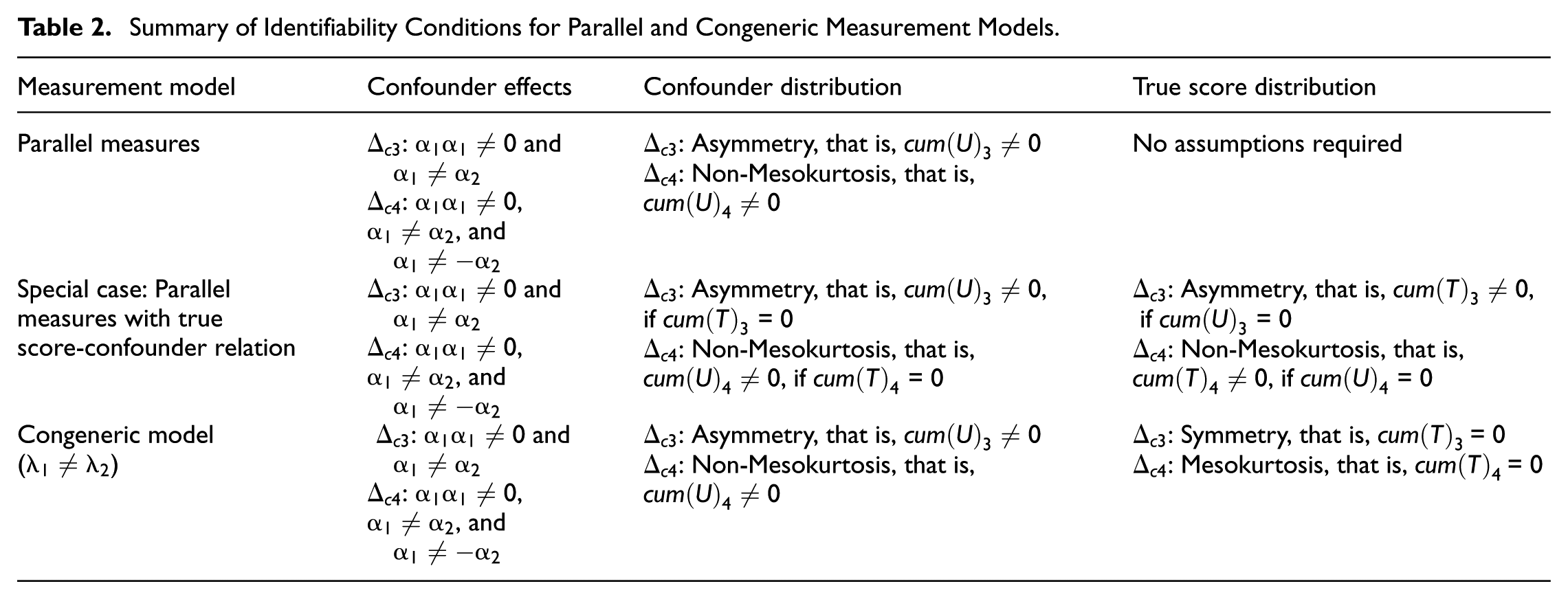
A summary of the identifiability conditions is given in Table 2. For all measurement models considered, confounder effect inequality constitutes a necessary condition, that is, ${\Delta }_{c3}$ requires that an active hidden confounder ( ${\alpha }_1{\alpha }_2\ne$ 0) influences X₁ and X₂ to unequal degrees ( ${\alpha }_1\ne {\alpha }_2$ ), whereas ${\Delta }_{c4}$ requires both, ${\alpha }_1\ne {\alpha }_2$ and ${\alpha }_1\ne -{\alpha }_2$ . In contrast, distributional requirements of T and U depend on the measurement model (parallel vs. congeneric models) and the structural influence of U. For truly parallel measures, non-Gaussianity of U (specifically, asymmetry for ${\Delta }_{c3}$ and non-mesokurtosis for ${\Delta }_{c4}$ ) is necessary when the hidden confounder influences X₁ and X₂ without any relation to the true scores T. In this case, no distributional assumptions are required for T. In contrast, when U is also related to T, non-Gaussianity of U is sufficient but not necessary when T deviates from Gaussianity. For congeneric models without any further information on factor loadings ( ${\lambda }_1$ and ${\lambda }_2$ ), non-Gaussianity of U (i.e., asymmetry for ${\Delta }_{c3}$ and non-mesokurtosis for ${\Delta }_{c4}$ ) and Gaussianity of T (symmetry for ${\Delta }_{c3}$ and mesokurtosis for ${\Delta }_{c4}$ ) are necessary to identify hidden confounding. ³

Table 2.

Summary of Identifiability Conditions for Parallel and Congeneric Measurement Models.

Measurement model	Confounder effects	Confounder distribution	True score distribution
Parallel measures	${\Delta }_{c3}$ : ${\alpha }_1{\alpha }_1\ne$ 0 and   ${\alpha }_1\ne {\alpha }_2$ ${\Delta }_{c4}$ : ${\alpha }_1{\alpha }_1\ne$ 0, ${\alpha }_1\ne {\alpha }_2$ , and   ${\alpha }_1\ne -{\alpha }_2$	${\Delta }_{c3}$ : Asymmetry, that is, $\mathrm{cum}{\left(U\right)}_3\ne$ 0 ${\Delta }_{c4}$ : Non-Mesokurtosis, that is, $\mathrm{cum}{\left(U\right)}_4\ne$ 0	No assumptions required
Special case: Parallel measures with true score-confounder relation	${\Delta }_{c3}$ : ${\alpha }_1{\alpha }_1\ne$ 0 and   ${\alpha }_1\ne {\alpha }_2$ ${\Delta }_{c4}$ : ${\alpha }_1{\alpha }_1\ne$ 0, ${\alpha }_1\ne {\alpha }_2$ , and   ${\alpha }_1\ne -{\alpha }_2$	${\Delta }_{c3}$ : Asymmetry, that is, $\mathrm{cum}{\left(U\right)}_3\ne$ 0, if $\mathrm{cum}{\left(T\right)}_3$ = 0 ${\Delta }_{c4}$ : Non-Mesokurtosis, that is, $\mathrm{cum}{\left(U\right)}_4\ne$ 0, if $\mathrm{cum}{\left(T\right)}_4$ = 0	${\Delta }_{c3}$ : Asymmetry, that is, $\mathrm{cum}{\left(T\right)}_3\ne$ 0, if $\mathrm{cum}{\left(U\right)}_3$ = 0 ${\Delta }_{c4}$ : Non-Mesokurtosis, that is, $\mathrm{cum}{\left(T\right)}_4\ne$ 0, if $\mathrm{cum}{\left(U\right)}_4$ = 0
Congeneric model ( ${\lambda }_1\ne {\lambda }_2$ )	${\Delta }_{c3}$ : ${\alpha }_1{\alpha }_1\ne$ 0 and   ${\alpha }_1\ne {\alpha }_2$ ${\Delta }_{c4}$ : ${\alpha }_1{\alpha }_1\ne$ 0, ${\alpha }_1\ne {\alpha }_2$ , and   ${\alpha }_1\ne -{\alpha }_2$	${\Delta }_{c3}$ : Asymmetry, that is, $\mathrm{cum}{\left(U\right)}_3\ne$ 0 ${\Delta }_{c4}$ : Non-Mesokurtosis, that is, $\mathrm{cum}{\left(U\right)}_4\ne$ 0	${\Delta }_{c3}$ : Symmetry, that is, $\mathrm{cum}{\left(T\right)}_3$ = 0 ${\Delta }_{c4}$ : Mesokurtosis, that is, $\mathrm{cum}{\left(T\right)}_4$ = 0

Based on these theoretical insights, questions concerning the plausibility of the required assumptions in practical applications naturally arise. Here, the requirement of confounder effect inequality finds empirical support when considering that, although both test forms may be affected by the examinee’s motivation, disengagement is more likely to exert a stronger influence on the second test than on the first (Wise & DeMars, 2005). Similarly, test anxiety tends to fluctuate over time and, thus, can have stronger effects on later tests, in particular, after perceived poor performance in the previous test (De Jonge et al., 2024). As another example, accumulated situational boredom can contaminate later measurements more strongly than earlier measurements (Eastwood et al., 2012). Furthermore, in all these examples, it can be considered highly unlikely that the causal effects from a common cause U on the observed measures would exactly flip signs (i.e., ${\alpha }_1=-{\alpha }_2$ ). However, although the requirement of unequal confounding influences in parallel measures seems plausible from a practical perspective, this assumption cannot be empirically tested and, therefore, requires theoretical justification.

Next, we focus on the non-Gaussianity requirements of ${\Delta }_{c3}$ and ${\Delta }_{c4}$ . Considering that non-Gaussianity is typically regarded as the rule rather than the exception in many educational and psychological settings (e.g., Micceri, 1989), distributional assumptions about U can be expected to be justifiable in practice. Even when conceptualizing U as an additive convolution of many hidden factors (Z. Chen & Chan, 2013; Wiedermann & von Eye, 2025), according to Cramér’s decomposition theorem (Cramér, 1970), the sum of independent influences cannot be exactly Gaussian, except all independent summands are exactly Gaussian. ⁴ However, despite the theoretical plausibility and empirical evidence of the ubiquitousness of non-Gaussianity, it is important to note that distributional requirements cannot be evaluated directly. An indirect examination is possible through evaluating distributional properties of X₁ and X₂ (e.g., using moment-specific significance tests such as D’Agostino’s (1971) skewness and Anscombe and Glynn’s (1983) kurtosis tests). However, these tests can only rule out (and not confirm) data requirements for ${\Delta }_{c3}$ and ${\Delta }_{c4}$ . That is, non-Gaussianity of X₁ and X₂ constitutes the minimum requirement to apply ${\Delta }_{c3}$ and ${\Delta }_{c4}$ in practice (the test statistics cannot be applied when X₁ and X₂ are in line with the Gaussian distribution). However, further distributional assumptions about U (and T when measures are congeneric) require theoretical justification.

Estimation of ${\mathbf{\Delta }}_{c3}$ and ${\mathbf{\Delta }}_{c4}$ and Statistical Inference

So far, we focused on population-level quantities, ${\Delta }_{c3}$ and ${\Delta }_{c4}$ . In practical applications with sample data, the population cumulants are replaced with their corresponding sample estimates. For example, in finite samples (of size N) with mean-centered measures X₁ and X₂, ${\Delta }_{c3}$ can be estimated via

$$\begin{array}{c}\multicolumn{1}{c}{{\hat{\mathrm{\Delta }}}_{c3}=\widehat{\mathrm{cum}}{(X_1,X_2)}_{12}-\widehat{\mathrm{cum}}{(X_1,X_2)}_{21}}\\ \multicolumn{1}{c}{=N^{-1}\sum X_1{X}_2^2-N^{-1}\sum X_1^2{X}_2}\end{array}$$

(18)

and non-parametric bootstrapping (e.g., sampling with replacement) can be used to obtain 95% confidence limits. Provided that distributional and confounder effect inequality assumptions given in Table 2 are fulfilled, one can conclude that the error independence assumption is violated when ${\hat{\mathrm{\Delta }}}_{c3}$ significantly differs from zero. Statistical tests based on ${\Delta }_{c4}$ can be constructed in a similar manner. That is,

$$\begin{array}{c}\multicolumn{1}{c}{{\hat{\mathrm{\Delta }}}_{c4}=\widehat{\mathrm{cum}}{(X_1,X_2)}_{13}-\widehat{\mathrm{cum}}{(X_1,X_2)}_{31}}\\ \multicolumn{1}{c}{=[N^{-1}\sum X_1{X}_2^3-3(N^{-1}\sum X_1{X}_2)(N^{-1}\sum X_2^2)]}\\ \multicolumn{1}{c}{-[N^{-1}\sum X_1^3{X}_2-3(N^{-1}\sum X_1{X}_2)(N^{-1}\sum X_1^2)]}\end{array}$$

(19)

can be used as a sample estimate, and resampling techniques can be applied to obtain 95% confidence intervals (CIs) for statistical inference. When ${\hat{\mathrm{\Delta }}}_{c4}$ significantly differs from zero, one has found evidence that the independent errors assumption is likely to be violated, provided that requirements given in Table 2 are fulfilled.

Monte-Carlo Simulation Experiments

To evaluate the performance of the proposed test statistics under various data conditions, we performed a series of Monte-Carlo simulation experiments. Monte-Carlo Simulation I focused on the performance of ${\Delta }_{c3}$ and ${\Delta }_{c4}$ in parallel measures with equal error variances. In Monte-Carlo Simulation II, we evaluated the behavior of ${\Delta }_{c3}$ and ${\Delta }_{c4}$ for parallel measures with true score-hidden confounder relations. Monte-Carlo Simulation III evaluated the finite sample behavior of the cumulant-based tests for τ-equivalent measures (i.e., under unequal error variances), and Monte-Carlo Simulation IV focused on the performance of ${\Delta }_{c3}$ and ${\Delta }_{c4}$ when measures are congeneric. All simulations were conducted in the R statistical programming environment (R Core Team, 2026). R code implementing the proposed test statistics is provided in the Online Supplement.

Monte-Carlo Simulation I: Performance of ${\mathbf{\Delta }}_{c3}$ and ${\mathbf{\Delta }}_{c4}$ for Parallel Measures

To evaluate the performance of the proposed test statistics for truly parallel measures, data were generated according to the data-generating mechanism given in Equation 3 with factor loadings fixed to one. That is, X₁ and X₂ were generated as a function of a common latent trait (T) and two error terms (E₁ and E₂). To induce systematic violations of the independent errors assumption, the two error terms were generated as a function of a common cause (U) and independent error-specific disturbances, W₁ and W₂. Exogenous variables (U and T) and error-specific disturbances (W₁ and W₂) were either sampled from the standard Gaussian distribution or various symmetric and asymmetric non-Gaussian populations with zero means. The population variances for U and T were set to be one. The population variances for W₁ and W₂ were chosen so that the standard deviations of E₁ and E₂ equaled 1.25. Asymmetrically distributed variables were generated from the Gamma distribution, and symmetric non-Gaussian variates were generated from the Johnson distribution (Johnson, 1949). Simulation factors systematically manipulated included the sample size (N), the distribution of the hidden confounder (U), the distribution of the latent trait (T), the distribution of the disturbances (W₁ and W₂), the ratio of confounder effects ( ${\alpha }_2/{\alpha }_1$ ), and the correlation between the error terms, cor(E₁, E₂):

Sample Size (N)

We considered three levels of sample sizes: 500, 1,000, and 5,000. The sample sizes we considered here represent a range of small to large samples in psychometrics (e.g., Golino & Epskamp, 2017) and non-Gaussian models (Wiedermann et al., 2023).

Distribution of Hidden Confounder (U)

The hidden confounder inducing non-independent error structures was either sampled from the standard Gaussian distribution (i.e., ${\gamma }_U$ = ${\delta }_U$ = 0), the Gamma distribution with skewness ${\gamma }_U$ = 0.75, 1.5, and 2.25 (mimicking mild, moderate, and severe asymmetry; Wiedermann et al., 2023), or symmetric Johnson distributions with excess-kurtosis ${\delta }_U$ = 2, 4, and 7 (mimicking mildly, moderately, and severely leptokurtic distributions; Shi et al., 2023). All distributions were generated with zero means and unit variances.

Distribution of the Latent Trait (T)

True scores were either sampled from the standard Gaussian distribution ( ${\gamma }_T$ = ${\delta }_T$ = 0), the Gamma distribution with a moderate skewness of ${\gamma }_T$ = 1.5, or the Johnson distribution with a moderate excess-kurtosis of ${\delta }_U$ = 4. All non-Gaussian distributions were generated exhibiting zero means and unit variances.

Distribution of Disturbances (W₁ and W₂)

The disturbance terms W₁ and W₂ were independently drawn from either a standard Gaussian population (i.e., ${\gamma }_{W_1}$ = ${\gamma }_{W_2}$ = ${\delta }_{W_1}$ = ${\delta }_{W_2}$ = 0), a Gamma distributed population with ${\gamma }_{W_1}$ = ${\gamma }_{W_2}$ = 1.5, or a symmetric Johnson distributed population with ${\delta }_{W_1}$ = ${\delta }_{W_2}$ = 4. All non-Gaussian distributions exhibited zero means and variances were set to guarantee equal standard deviations of the error terms E₁ and E₂ (with ${\sigma }_{E_1}$ = ${\sigma }_{E_2}$ = 1.25).

Ratio of Confounder Effects ( $R={\alpha }_2/{\alpha }_1$ )

The ratio of coefficients of the confounder paths were set to $R={\alpha }_2/{\alpha }_1$ = 1, 1.25, 2, and 2.5. Here, $R$ = 1 mimics cases in which the cumulant-based test statistics cannot be expected to detect non-independent error structures. In contrast, $R$ > 1 constitute data cases where non-independent errors can be detected using the proposed test statistics.

Correlation Between Errors

We manipulated the correlations between the error terms, cor(E₁, E₂), at three levels: 0.19, 0.38, and 0.48. The assumption of independent errors is violated to a greater degree as the magnitude of the correlation coefficient increases. These levels of correlation approximate small, medium, and nearly large effect sizes, based on Cohen’s guidelines (Cohen, 1988). Note that the population values of the paths ${\alpha }_1$ and ${\alpha }_2$ are determined by the population parameters specified above. For example, when ${\sigma }_{E_1}$ = ${\sigma }_{E_2}$ = 1.25 and cor(E₁, E₂) = 0.19, then $\frac{{\alpha }_1{\alpha }_2}{1.25\times 1.25}$ = 0.19. If we additionally set ${\alpha }_2/{\alpha }_1$ = 1.25, the population values of ${\alpha }_1$ and ${\alpha }_2$ can be uniquely determined by solving these two equations.

In total, for each type of non-Gaussian population (symmetric Johnson vs. asymmetric Gamma distributions), the simulation design was fully crossed leading to 3 × 4 × 2 × 2 × 3 × 4 = 576 simulation conditions. ⁵ However, 48 conditions were inadmissible (when ${\alpha }_1{\alpha }_2$ = 0.75 and ${\alpha }_2/{\alpha }_1$ = 2.5) resulting in 576 – 48 = 528 simulation conditions for each type of non-Gaussianity, and 528 × 2 = 1056 simulation conditions in total. For each simulation condition, 500 replications were generated. For each generated variable pair, X₁ and X₂, we computed the test statistics ${\Delta }_{c3}$ and ${\Delta }_{c4}$ and used non-parametric bootstrapping (sampling with replacement) to construct 95% percentile bootstrap confidence intervals (with 2,000 resamples). Test statistics significantly different from zero indicate a violation of the independent errors assumption.

Results

In the following sections, we present the results of the Monte-Carlo experiment. For reasons of comparability, we separately report simulation results for cases of equal (i.e., R = 1) and unequal (R > 1) magnitudes of confounding effects.

Equal Magnitudes of Confounding Effects

Tables 3 and 4 give the proportion of significant results of ${\Delta }_{c3}$ and ${\Delta }_{c4}$ for asymmetric and symmetric non-Gaussian populations with identical path coefficients, that is, R = ${\alpha }_2$ / ${\alpha }_1$ = 1. Because both cumulant-based test statistics require R > 1 to detect non-independent errors regardless of the distribution of the common cause U, the proportions of significant results represent observed Type I error rates. Overall, Type I error rates for ${\Delta }_{c3}$ are in good accordance with Bradley’s (1978) liberal robustness criterion ⁶ regardless of sample size, error correlation, and magnitude of asymmetry of the confounder U, the true scores T, and random disturbances W₁ and W₂ (inflated Type I errors occur in only 6.3% of the asymmetric conditions and in 3.5% of the symmetric non-Gaussian conditions). In contrast, inflated Type I error rates (> 7.5%) occur more often for ${\Delta }_{c4}$ (18.1% of the asymmetric and 16.7% of the symmetric non-Gaussian conditions). Thus, overall, we can conclude that simulation results confirm our theoretical findings and underline the importance of inequality of confounding effects to detect violations of the assumption of independent errors.

Table 3.

Type I Errors of ${\Delta }_{c3}$ and ${\Delta }_{c4}$ for Asymmetrically Distributed Populations When R = 1. Inflated Type I Errors Larger Than 7.5% Are Marked Bold.

				cor(E1, E2) = 0.19		cor(E1, E2) = 0.38		cor(E1, E2) = 0.48
N	${\gamma }_U$	${\gamma }_T$	${\gamma }_W$	${\Delta }_{c3}$	${\Delta }_{c4}$	${\Delta }_{c3}$	${\Delta }_{c4}$	${\Delta }_{c3}$	${\Delta }_{c4}$
500	0	0	0	0.056	0.056	0.060	0.062	0.056	0.058
500	0	0	1.5	0.074	0.082	0.076	0.062	0.058	0.054
500	0	1.5	0	0.076	0.080	0.050	0.064	0.072	0.072
500	0	1.5	1.5	0.078	0.088	0.072	0.070	0.044	0.056
500	0.75	0	0	0.042	0.050	0.052	0.050	0.064	0.062
500	0.75	0	1.5	0.058	0.076	0.070	0.060	0.054	0.046
500	0.75	1.5	0	0.072	0.066	0.052	0.054	0.054	0.082
500	0.75	1.5	1.5	0.046	0.046	0.066	0.068	0.064	0.060
500	1.5	0	0	0.048	0.044	0.054	0.068	0.070	0.066
500	1.5	0	1.5	0.048	0.076	0.070	0.074	0.046	0.052
500	1.5	1.5	0	0.044	0.062	0.050	0.048	0.052	0.080
500	1.5	1.5	1.5	0.052	0.058	0.070	0.074	0.060	0.052
500	2.25	0	0	0.030	0.056	0.068	0.090	0.078	0.064
500	2.25	0	1.5	0.066	0.068	0.082	0.094	0.052	0.060
500	2.25	1.5	0	0.046	0.066	0.056	0.080	0.046	0.068
500	2.25	1.5	1.5	0.058	0.074	0.066	0.080	0.058	0.072
1,000	0	0	0	0.066	0.042	0.048	0.072	0.050	0.062
1,000	0	0	1.5	0.040	0.044	0.050	0.064	0.068	0.064
1,000	0	1.5	0	0.054	0.058	0.056	0.064	0.058	0.070
1,000	0	1.5	1.5	0.086	0.084	0.052	0.048	0.080	0.064
1,000	0.75	0	0	0.044	0.062	0.058	0.062	0.076	0.062
1,000	0.75	0	1.5	0.070	0.092	0.040	0.076	0.062	0.078
1,000	0.75	1.5	0	0.054	0.068	0.046	0.066	0.074	0.074
1,000	0.75	1.5	1.5	0.058	0.072	0.072	0.058	0.042	0.070
1,000	1.5	0	0	0.052	0.046	0.062	0.060	0.056	0.066
1,000	1.5	0	1.5	0.068	0.076	0.062	0.072	0.054	0.054
1,000	1.5	1.5	0	0.062	0.076	0.058	0.082	0.072	0.064
1,000	1.5	1.5	1.5	0.052	0.056	0.044	0.068	0.052	0.064
1,000	2.25	0	0	0.050	0.054	0.060	0.056	0.054	0.062
1,000	2.25	0	1.5	0.062	0.062	0.068	0.074	0.054	0.086
1,000	2.25	1.5	0	0.054	0.058	0.054	0.068	0.074	0.080
1,000	2.25	1.5	1.5	0.062	0.054	0.052	0.092	0.072	0.076
5,000	0	0	0	0.028	0.046	0.066	0.038	0.052	0.038
5,000	0	0	1.5	0.044	0.068	0.060	0.066	0.048	0.070
5,000	0	1.5	0	0.048	0.054	0.048	0.058	0.054	0.042
5,000	0	1.5	1.5	0.042	0.050	0.046	0.062	0.046	0.032
5,000	0.75	0	0	0.034	0.054	0.048	0.050	0.042	0.060
5,000	0.75	0	1.5	0.046	0.046	0.062	0.046	0.050	0.070
5,000	0.75	1.5	0	0.034	0.046	0.048	0.058	0.056	0.052
5,000	0.75	1.5	1.5	0.076	0.074	0.066	0.086	0.048	0.046
5,000	1.5	0	0	0.046	0.060	0.070	0.062	0.048	0.080
5,000	1.5	0	1.5	0.052	0.066	0.042	0.056	0.038	0.064
5,000	1.5	1.5	0	0.046	0.048	0.060	0.072	0.044	0.058
5,000	1.5	1.5	1.5	0.048	0.078	0.060	0.060	0.052	0.064
5,000	2.25	0	0	0.056	0.050	0.060	0.070	0.058	0.056
5,000	2.25	0	1.5	0.036	0.052	0.066	0.074	0.044	0.052
5,000	2.25	1.5	0	0.052	0.064	0.056	0.076	0.072	0.060
5,000	2.25	1.5	1.5	0.054	0.058	0.046	0.048	0.064	0.070

Table 4.

Type I Errors of ${\Delta }_{c3}$ and ${\Delta }_{c4}$ for Symmetrically Non-Gaussian Populations When R = 1. Inflated Type I Errors Larger Than 7.5% Are Marked Bold.

				cor(E1, E2) = 0.19		cor(E1, E2) = 0.38		cor(E1, E2) = 0.48
N	${\delta }_U$	${\delta }_T$	${\delta }_W$	${\Delta }_{c3}$	${\Delta }_{c4}$	${\Delta }_{c3}$	${\Delta }_{c4}$	${\Delta }_{c3}$	${\Delta }_{c4}$
500	0	0	0	0.040	0.046	0.074	0.048	0.052	0.078
500	0	0	4	0.060	0.074	0.072	0.074	0.060	0.064
500	0	4	0	0.056	0.060	0.066	0.062	0.060	0.076
500	0	4	4	0.040	0.066	0.064	0.074	0.070	0.072
500	2	0	0	0.052	0.056	0.064	0.060	0.070	0.068
500	2	0	4	0.056	0.054	0.054	0.064	0.062	0.070
500	2	4	0	0.058	0.058	0.074	0.070	0.062	0.066
500	2	4	4	0.066	0.062	0.070	0.094	0.056	0.066
500	4	0	0	0.060	0.068	0.076	0.076	0.054	0.072
500	4	0	4	0.062	0.074	0.060	0.086	0.062	0.070
500	4	4	0	0.068	0.070	0.056	0.074	0.074	0.068
500	4	4	4	0.048	0.054	0.072	0.068	0.052	0.066
500	7	0	0	0.056	0.058	0.072	0.066	0.046	0.078
500	7	0	4	0.056	0.074	0.060	0.074	0.050	0.062
500	7	4	0	0.046	0.072	0.044	0.062	0.052	0.074
500	7	4	4	0.052	0.064	0.072	0.078	0.044	0.078
1,000	0	0	0	0.054	0.076	0.044	0.050	0.052	0.034
1,000	0	0	4	0.062	0.074	0.086	0.078	0.046	0.054
1,000	0	4	0	0.084	0.066	0.060	0.058	0.074	0.058
1,000	0	4	4	0.070	0.060	0.072	0.066	0.040	0.066
1,000	2	0	0	0.044	0.046	0.044	0.060	0.052	0.064
1,000	2	0	4	0.064	0.078	0.050	0.054	0.074	0.060
1,000	2	4	0	0.050	0.048	0.052	0.056	0.046	0.064
1,000	2	4	4	0.056	0.062	0.062	0.066	0.060	0.072
1,000	4	0	0	0.060	0.058	0.062	0.060	0.054	0.060
1,000	4	0	4	0.066	0.084	0.072	0.080	0.070	0.054
1,000	4	4	0	0.036	0.088	0.060	0.074	0.076	0.046
1,000	4	4	4	0.066	0.084	0.066	0.074	0.060	0.060
1,000	7	0	0	0.034	0.048	0.062	0.072	0.042	0.082
1,000	7	0	4	0.050	0.050	0.054	0.050	0.062	0.046
1,000	7	4	0	0.068	0.064	0.056	0.084	0.060	0.048
1,000	7	4	4	0.058	0.080	0.086	0.062	0.048	0.046
5,000	0	0	0	0.056	0.050	0.036	0.058	0.064	0.054
5,000	0	0	4	0.058	0.062	0.042	0.044	0.058	0.046
5,000	0	4	0	0.048	0.058	0.060	0.060	0.046	0.054
5,000	0	4	4	0.064	0.072	0.034	0.046	0.050	0.080
5,000	2	0	0	0.038	0.038	0.044	0.054	0.044	0.060
5,000	2	0	4	0.054	0.056	0.048	0.062	0.052	0.064
5,000	2	4	0	0.058	0.044	0.052	0.074	0.054	0.078
5,000	2	4	4	0.064	0.072	0.068	0.102	0.044	0.050
5,000	4	0	0	0.048	0.046	0.058	0.046	0.044	0.054
5,000	4	0	4	0.044	0.058	0.034	0.068	0.058	0.046
5,000	4	4	0	0.050	0.056	0.058	0.060	0.042	0.046
5,000	4	4	4	0.060	0.074	0.060	0.068	0.064	0.046
5,000	7	0	0	0.054	0.070	0.040	0.068	0.042	0.060
5,000	7	0	4	0.058	0.060	0.048	0.058	0.034	0.064
5,000	7	4	0	0.050	0.040	0.042	0.080	0.058	0.080
5,000	7	4	4	0.052	0.058	0.054	0.088	0.054	0.062

Unequal Magnitudes of Confounding Effects

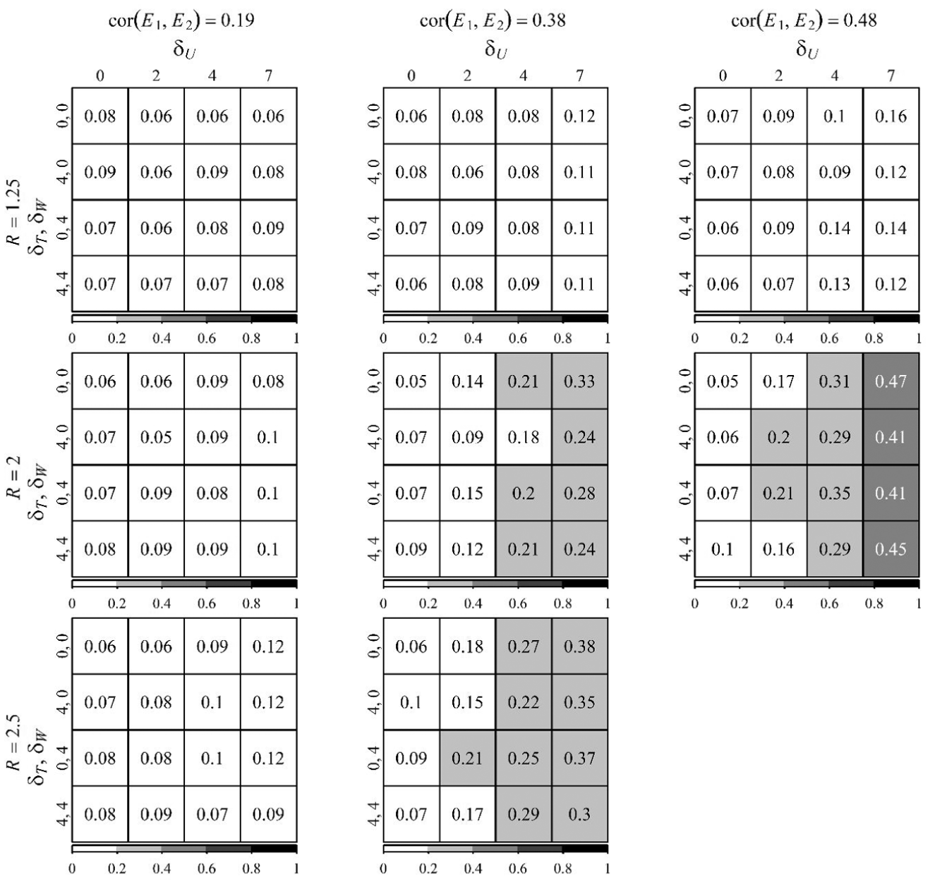
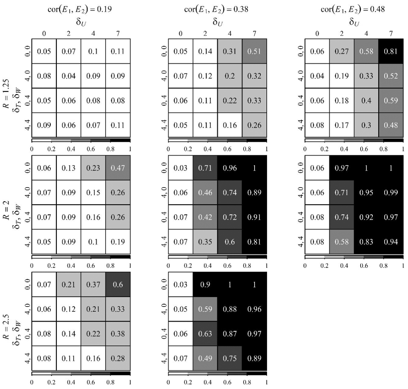
Next, we focus on cases where the requirement of inequality of confounding effects is fulfilled (R > 1). Here, two important distinctions must be made: First, when the common cause U follows a Gaussian distribution, the cumulant-based test statistics cannot be expected to detect violations of the independent errors assumption due to the absence of a T-U relation (cf. Table 2). Thus, in these cases, the proportions of rejected null hypotheses of ${\Delta }_{c3}$ and ${\Delta }_{c4}$ reflect Type I error rates. Second, when U deviates from Gaussianity, we can expect that cumulant-based test statistics reject the null hypothesis and, thus, indicate the presence of non-independent errors. In other words, these data cases reflect the statistical power of ${\Delta }_{c3}$ and ${\Delta }_{c4}$ . Furthermore, the present simulation design allows one to evaluate the isolated effects of the various sources of non-Gaussianity of X₁ and X₂ on ${\Delta }_{c3}$ and ${\Delta }_{c4}$ , that is, cases in which only one of the exogeneous variables (T, U, W₁, and W₂) deviates from Gaussianity. For comparability, we report the results separately for asymmetric and symmetric non-Gaussian populations. Figures 2 to 4 summarize the empirical Type I error rates (i.e., when ${\gamma }_U$ = 0) and the power of ${\Delta }_{c3}$ to detect violations of the independent errors assumption when variables are drawn from various asymmetric distributions. Figures 5 to 7 summarize the empirical Type I error rates (i.e., when ${\delta }_U$ = 0) and the power of ${\Delta }_{c4}$ for symmetric non-Gaussian populations.

Figure 2.

Proportion of rejected null hypotheses of ${\Delta }_{c3}$ as a function of error correlation [cor(E₁, E₂)], skewness of true scores ( ${\gamma }_T$ ), hidden confounders ( ${\gamma }_U$ ), random disturbances ( ${\gamma }_{W_1}$ = ${\gamma }_{W_2}$ = ${\gamma }_W$ ), and inequality of confounding effects (R) for N = 500 observations. The cell entries reflect Type I error rates when ${\gamma }_U$ = 0 and statistical power rates to detect correlated errors when ${\gamma }_U$ > 0.

Figure 3.

Proportion of rejected null hypotheses of ${\Delta }_{c3}$ as a function of error correlation [cor(E₁, E₂)], skewness of true scores ( ${\gamma }_T$ ), hidden confounders ( ${\gamma }_U$ ), random disturbances ( ${\gamma }_{W_1}$ = ${\gamma }_{W_2}$ = ${\gamma }_W$ ), and inequality of confounding effects (R) for N = 1,000 observations. The cell entries reflect Type I error rates when ${\gamma }_U$ = 0 and statistical power rates to detect correlated errors when ${\gamma }_U$ > 0.

Figure 4.

Proportion of rejected null hypotheses of ${\Delta }_{c3}$ as a function of error correlation [cor(E₁, E₂)], skewness of true scores ( ${\gamma }_T$ ), hidden confounders ( ${\gamma }_U$ ), random disturbances ( ${\gamma }_{W_1}$ = ${\gamma }_{W_2}$ = ${\gamma }_W$ ), and inequality of confounding effects (R) for N = 5,000 observations. The cell entries reflect Type I error rates when ${\gamma }_U$ = 0 and statistical power rates to detect correlated errors when ${\gamma }_U$ > 0.

Figure 5.

Proportion of rejected null hypotheses of ${\Delta }_{c4}$ as a function of error correlation [cor(E₁, E₂)], excess-kurtosis of true scores ( ${\delta }_T$ ), hidden confounders ( ${\delta }_U$ ), random disturbances ( ${\delta }_{W_1}$ = ${\delta }_{W_2}$ = ${\delta }_W$ ), and inequality of confounding effects (R) for N = 500 observations. The cell entries reflect Type I error rates when ${\delta }_U$ = 0 and statistical power rates to detect correlated errors when ${\delta }_U$ > 0.

Figure 6.

Proportion of rejected null hypotheses of ${\Delta }_{c4}$ as a function of error correlation [cor(E₁, E₂)], excess-kurtosis of true scores ( ${\delta }_T$ ), hidden confounders ( ${\delta }_U$ ), random disturbances ( ${\delta }_{W_1}$ = ${\delta }_{W_2}$ = ${\delta }_W$ ), and inequality of confounding effects (R) for N = 1,000 observations. The cell entries reflect Type I error rates when ${\delta }_U$ = 0 and statistical power rates to detect correlated errors when ${\delta }_U$ > 0.

Figure 7.

Statistical power of ${\Delta }_{c4}$ to detect correlated errors in parallel measures as a function of error correlation [cor(E₁, E₂)], excess-kurtosis of true scores (), hidden confounders ( ${\delta }_U$ ), random disturbances ( ${\delta }_{W_1}$ = ${\delta }_{W_2}$ = ${\delta }_W$ ), and inequality of confounding effects (R) for N = 5,000 observations. The cell entries reflect Type I error rates when ${\delta }_U$ = 0 and statistical power rates to detect correlated errors when ${\delta }_U$ > 0.

In the first step, we summarize the behavior of ${\Delta }_{c3}$ when only one of the exogenous variables (T, U, W₁, and W₂) deviates from Gaussianity. When the latent trait is the only source of non-Gaussianity (i.e., cases in which ${\gamma }_T\ne$ 0 and ${\gamma }_U$ = ${\gamma }_{W_1}$ = ${\gamma }_{W_2}$ = 0), the proportion of significant ${\Delta }_{c3}$ estimates closely corresponds to the nominal significance level of 5%, independent of the error correlation, inequality of confounding effects, and sample size. Similar effects can be observed for data scenarios in which the random disturbances (W₁ and W₂) provide the only source of non-Gaussianity (i.e., ${\gamma }_T$ = ${\gamma }_U$ = 0 and ${\gamma }_{W_1}={\gamma }_{W_2}$ ≠ 0), that is, again, rejection rates of ${\Delta }_{c3}$ are close to the 5% significance threshold. When U constitutes the only non-Gaussian component in the variable system (i.e., ${\gamma }_U\ne$ 0 and ${\gamma }_T$ = ${\gamma }_{W_1}$ = ${\gamma }_{W_2}$ = 0), rejection rates of ${\Delta }_{c3}$ systematically increase with the skewness of U. For small sample sizes (N = 500), rejection rates exceed 80%, when R = 2, cor(E₁, E₂) = 0.48, and ${\gamma }_U$ ≥ 1.5 or when R = 2.5, cor(E₁, E₂) = 0.38, and ${\gamma }_U$ = 2.25. For moderate sample sizes (N = 1,000), rejection rates exceed 80%, when R≥ 2 and cor(E₁, E₂) ≥ 0.38. When samples are large (N = 5,000), small error correlations (i.e., cor(E₁, E₂) = 0.19) can be detected with a power > 80% for heavily skewed confounders ( ${\gamma }_U$ = 2.25) and moderate to large confounder effect inequalities. When error correlations are moderate to large (i.e., cor(E₁, E₂) ≥ 0.38) even small deviations from Gaussianity of U tend to be sufficient to achieve acceptable power, provided that confounder effect inequalities are at least moderate (R≥ 2).

Next, we focus on the joint effects of the considered simulation factors. For ${\gamma }_U$ = 0, the test statistic ${\Delta }_{c3}$ shows adequate Type I error protection regardless of the sample size, the distributions of T, W₁, and W₂, and the inequality of confounding effects (R). In contrast, when ${\gamma }_U$ > 0, as expected, the power of ${\Delta }_{c3}$ increases with the sample size, the magnitude of asymmetry of the hidden confounder U, and the ratio of confounding effects R. In contrast, the power tends to decrease with the skewness of the true scores T and the disturbances W₁ and W₂. In other words, the power of ${\Delta }_{c3}$ to detect non-independent error structures tends to be higher when the hidden confounder constitutes the only source of asymmetry. Furthermore, when the error correlation is small (i.e., cor(E₁, E₂) = 0.19) and the confounding effect ratio is close to 1 (i.e., R = 1.25), the ${\Delta }_{c3}$ statistic does not have sufficient power regardless of the magnitude of skewness of the confounder, the true scores, and the random disturbances, and the sample sizes considered. For N = 500, highly skewed hidden confounders and R = 2.5 are required to detect moderately correlated errors (cor(E₁, E₂) = 0.38) with a statistical power > 80%. In contrast, for N = 1,000, depending on the degree of asymmetry of T, W₁, and W₂ (power increases when distributions are close to symmetry), at least moderately skewed confounding (i.e., ${\gamma }_U$ ≥ 1.5) is sufficient to obtain a power ≥ 80%. When sample sizes are large (N = 5,000), even small error correlations (cor(E₁, E₂) = 0.19) can be detected with sufficient power when the confounder is heavily skewed ( ${\gamma }_U$ = 2.25) and R = 2, and moderate to large violations of the independent error assumption are detectable for slightly skewed confounders ( ${\gamma }_U$ = 0.75) and R = 2 or highly skewed confounders and mild inequality of confounding effects (R = 1.25).

Next, we focus on the statistical performance of Δ_c4 when population variables are symmetric and non-Gaussian. Figures 5 to 7 summarize the proportion of rejecting the null hypothesis H₀: ${\Delta }_{c4}$ = 0 as a function of the error correlation, the excess-kurtosis of the confounder, the true scores, and the random disturbances ( ${\delta }_U$ , ${\delta }_T$ , and ${\delta }_{W_1}$ = ${\delta }_{W_2}$ = ${\delta }_W$ ), and the magnitude of inequality of confounding effects (R) for N = 500, 1,000, and 5,000, respectively. Again, the proportions of rejected null hypotheses reflect empirical Type I error rates when ${\delta }_U$ = 0 and the statistical power when ${\delta }_U$ > 0.

First, we start with summarizing the behavior of ${\Delta }_{c4}$ when only one of the exogenous variables (T, U, W₁, and W₂) deviates from Gaussianity. When the latent trait T constitutes the only source of non-Gaussianity, the proportions of significant ${\Delta }_{c4}$ estimates fall below the robustness threshold of 7.5% in the majority of cases. However, rejection rates up to 10% can occur for small samples (N = 500), when cor(E₁, E₂) = 0.38 and R = 2.5, and for moderate sample sizes (N = 1,000), when cor(E₁, E₂) = 0.48 and R = 2. When the hidden confounder U is the only exogenous variable that deviates from Gaussianity, rejection rates of H₀: ${\Delta }_{c4}$ = 0 systematically increase with the excess-kurtosis of U, as expected. However, acceptable power rates > 80% generally require large sample sizes (N = 5,000). For small confounder effect inequalities (R = 1.25), heavily leptokurtic confounders ( ${\delta }_U$ = 7) are needed. When confounder effect inequality is moderate (R = 2), ${\delta }_U\ge$ 4 is sufficient to detect moderate error correlations (cor(E₁, E₂) = 0.38), and small deviations from Gaussianity ( ${\delta }_U\ge$ 2) are enough to detect large error correlations (cor(E₁, E₂) = 0.48). Finally, when random disturbances (W₁ and W₂) provide the only source of non-Gaussianity, the proportions of significant ${\Delta }_{c4}$ estimates, again, fall below the robustness threshold of 7.5% in the majority of cases. However, for small to moderate samples (N = 500 and 1,000), moderately correlated errors (i.e., cor(E₁, E₂) = 0.38), and large confounder effect inequalities (R = 2.5), rejection rates up to 9% are observed.

In the last step, we focus on the joint effects of the simulation factors on the performance of ${\Delta }_{c4}$ . For leptokurtic common causes ( ${\delta }_U$ > 0), small samples (N = 500) are not sufficient to achieve acceptable power regardless of the considered levels of the remaining simulation factors. Even for large error correlations together with R = 2, power rates only range from 41% to 47% (cf. Figure 5). Similarly, for N = 1,000, highly leptokurtic confounders (i.e., ${\delta }_U$ = 7), a confounder effect inequality of R = 2, and Gaussian true scores and random disturbances are required to achieve a statistical power of 77% (cf. Figure 6). When sample sizes are large (N = 5,000), the power of ${\Delta }_{c4}$ exceeds 80% for detecting moderately correlated errors (cor(E₁, E₂) = 0.38) when the confounder is heavily leptokurtic (i.e., ${\delta }_U$ = 7) and the ratio of confounding effects equals R = 2, and slightly leptokurtic confounders ( ${\delta }_U$ = 2) are sufficient when confounding effects heavily differ from each other (i.e., R = 2.5) and true scores and random disturbances are mesokurtic (i.e., Gaussian). In a way similar to ${\Delta }_{c3}$ , the statistical power of ${\Delta }_{c4}$ . decreases with non-Gaussianity of the latent trait (T) and the random disturbances (W₁ and W₂).

Monte-Carlo Simulation II: True Score-Confounder Relation

So far, we assumed that true scores (T) and hidden confounders (U) are independent of each other. As systematic relations between T and U may occur in practical applications, we further investigated the effects of true score-confounder correlations on the behavior of ${\Delta }_{c3}$ and ${\Delta }_{c4}$ . Here, theoretical results suggest that both test statistics can be expected to attain zero when confounding effects are equal ( ${\alpha }_1$ = ${\alpha }_2$ ) and deviate from zero when confounding effects are unequal. Furthermore, in contrast to the case of uncorrelated true scores and confounders, due to non-vanishing higher order cross-moments of T and U, ${\Delta }_{c3}\ne$ 0 and ${\Delta }_{c4}\ne$ 0 can also be expected when U is Gaussian and true scores are non-Gaussian.

To validate these theoretical findings and to assess the finite sample performance of ${\Delta }_{c3}$ and ${\Delta }_{c4}$ when true scores and hidden confounders are correlated, a Monte-Carlo simulation was performed where data were generated according to the parallel measures model with equal factor loadings. For simplicity, the simulation experiment was restricted to asymmetrically distributed populations. The simulation design systematically varied the degree of confounder skewness ( ${\gamma }_U$ = 0, 0.75, 1.5, 2.25), the skewness of random disturbances ( ${\gamma }_{W_1}$ = ${\gamma }_{W_2}$ = 0, 1.5), confounder-true score correlations (cor(T, U) = 0.2, 0.5), confounder effect inequalities (R = α₂/α₁ = 1, 1.25, 2, and 2.5), error correlations (cor(E₁, E₂) = 0.19, 0.38, and 0.48), and sample sizes (N = 500, 1,000, 5,000), resulting in 528 admissible simulation conditions (with 500 iterations per condition). For each condition, ${\Delta }_{c3}$ and ${\Delta }_{c4}$ estimates were evaluated using percentile bootstrap confidence intervals based on 2,000 resamples (further details are given in the section “Monte-Carlo Simulation II: True Score-Confounder Relation” in the Online Supplement).

Results

The present section summarizes the simulation results with respect to the Type I error and power behavior of the two test statistics. Detailed results are presented in the Online Supplemental Material of the article.

Equal Magnitudes of Confounding Effects

When confounding effects were equal (R ;= 1), rejection rates reflect Type I errors. Simulation results (cf. Tables S1 in the Online Supplement) confirm that ${\Delta }_{c3}$ consistently maintains the nominal 5% significance level regardless of the magnitude of cor(T, U), distributional shapes of confounders and random disturbances, error correlations, and sample size. In contrast, again, ${\Delta }_{c4}$ tends to be too liberal for small samples but performs adequately when sample sizes are large. Overall, compared to the case of independent true scores and confounders, we can conclude that correlations between T and U do not further distort the Type I error behavior of the test statistics.

Unequal Magnitudes of Confounding Effects

When confounding effects are unequal (R > 1), the power to detect non-independent errors of both cumulant-based tests increases with the non-Gaussianity of the hidden confounder, the degree of confounder effect inequality, and sample size, as expected. For ${\Delta }_{c3}$ , power also increases with stronger correlations between true scores and confounders, while skewness in measurement disturbances (W₁ and W₂) reduces power mainly in smaller samples (cf. Figures S1–S3 in the Online Supplement). Notably, when true scores and confounders are correlated, ${\Delta }_{c3}$ can detect non-independent errors even when the confounder is Gaussian, provided that true scores are skewed and confounding effects differ in magnitude. In large samples with strong confounder effect inequality, power exceeds 80%.

${\Delta }_{c4}$ shows similar power patterns (see Figures S4–S6 in the Online Supplement). That is, ${\Delta }_{c4}$ benefits from larger confounder excess-kurtosis, unequal confounding effects, larger samples, mesokurtic disturbances, and correlated true scores and confounders. However, its power is generally lower than that of ${\Delta }_{c3}$ , indicating that ${\Delta }_{c3}$ should be preferred when variables are asymmetric. Overall, simulation evidence confirms the theoretical results and suggests that correlated true scores and confounders extend the parameter space under which the cumulant-based tests can be used to detect non-independent error structures.

Monte-Carlo Simulation III: Influence of Unequal Error Variances

In deriving the test statistics ${\Delta }_{c3}$ and ${\Delta }_{c4}$ , we did not assume equal error variances. Thus, the test statistics, in theory, are applicable to both parallel and τ-equivalent measures. To assess their finite sample performance under τ-equivalence with unequal error variances, a Monte-Carlo simulation was conducted in which X₁ and X₂ exhibit equal loadings (i.e., λ₁ = λ₂) but different error variances ( ${\sigma }_{E_1}^2\ne {\sigma }_{E_2}^2$ ). Data were generated under various distributions of true scores ( ${\gamma }_T$ = 0 or 1.5; ${\delta }_T$ = 0 or 4), hidden confounders ( ${\gamma }_U$ = 0, 0.75, 1.5, and 2.25; ${\delta }_U$ = 0, 2, 4, and 7), and independent disturbances ( ${\gamma }_{W_1}$ = ${\gamma }_{W_2}$ = 0 or 1.5; ${\delta }_{W_1}$ = ${\delta }_{W_2}$ = 0 or 4), different ratios of confounding effects (R = α₂/α₁ = 1, 1.25, 2, and 2.5), fixed levels of correlated errors (i.e., cor(E₁, E₂) = 0.23 or 0.47), and sample sizes of N = 500, 1,000, and 5,000. Error variances were set such that variability in E₂ was twice the variability of E₁ (with ${\sigma }_{E_1}$ = 0.8 and ${\sigma }_{E_2}$ = 1.6). The fully crossed design consisted of 384 conditions. Each condition was replicated 500 times and each X₁-X₂ pair was evaluated using ${\Delta }_{c3}$ and ${\Delta }_{c4}$ with 95% percentile bootstrap confidence intervals based on 2,000 resamples (further details are given in the section “Monte-Carlo Simulation III: Unequal Error Variances” in the Online Supplement).

Results

Equal Magnitudes of Confounding Effects

Because factor loadings of the parallel measures were identical, cases of equal confounding effects (R = 1) constitute data situations in which one expects that rejection rates of ${\Delta }_{c3}$ and ${\Delta }_{c4}$ are close to the nominal significance level of 5%. Tables S2 and S3 of the Online Supplement summarize the empirical Type I error rates for both test statistics. Results suggest that ${\Delta }_{c3}$ largely maintains the nominal 5% Type I error rate, even under skewed or symmetric non-Gaussian distributions. In contrast, ${\Delta }_{c4}$ is frequently too liberal in statistical decisions, with Type I error rates up to 15%. For asymmetric populations, Type I error rates exceeded the robustness threshold in 73% of the cases, for symmetric non-Gaussian populations, 70% of the empirical Type I error rates exceeded the 7.5% robustness threshold. Thus, although the cumulant-based test statistics do, in theory, not rely on the assumption of equal error variances, ${\Delta }_{c4}$ is sensitive to unequal error variances in terms of statistical decision making.

Unequal Magnitudes of Confounding Effects

Figures S7 to S10 in the Online Supplement summarize the finite sample behavior of ${\Delta }_{c3}$ and ${\Delta }_{c4}$ when confounding effects are unequal (R > 1). Here, both ${\Delta }_{c3}$ and ${\Delta }_{c4}$ can be expected to reject the null hypothesis when the hidden confounder is non-Gaussian. For ${\Delta }_{c3}$ (cf. Figures S7 and S8 in the Online Supplement), power increases with the skewness of the confounder, the inequality in confounding effects, the sample size, and the magnitude of error correlation, but decreases with non-Gaussianity in true scores and disturbances. Compared with the equal-error-variance case, heterogeneous error variances generally reduce the statistical power. For small error correlations, high statistical power (>80%) is achieved only under sufficiently large samples, large confounder effect inequality, and strongly asymmetric confounders. For large error correlations, either small sample sizes and heavily skewed confounders with highly unequal confounding influences or moderate to large sample sizes with at least moderately skewed confounders are necessary to achieve acceptable statistical power. For large sample sizes and confounder effect inequalities R≥ 2, adequate statistical power can be observed even when hidden confounders only slightly deviate from symmetry.

For ${\Delta }_{c4}$ under symmetric non-Gaussian distributions (cf. Figures S9 and S10 in the Online Supplement), power increases with confounder excess-kurtosis, confounder effect inequality, and sample size, but is reduced by non-Gaussian true scores and random disturbances, and by unequal error variances. As a result, ${\Delta }_{c4}$ exhibits low power (< 80%) for small error correlations across all conditions and requires large samples and moderately to strongly non-Gaussian confounders to attain acceptable power when error correlations are large.

Monte-Carlo Simulation IV: Influence of Unequal Factor Loadings

The presented theoretical findings indicate that equality of factor loadings constitutes a critical condition for detecting error non-independence due to hidden confounding, in particular, when additional distributional assumptions about the latent trait cannot be defended. To assess the consequences of violating this condition, we repeated Simulation Study I under unequal factor loadings, considering both asymmetric and symmetric non-Gaussian distributions. Data were generated according to the congeneric model given in Equation 3. Factor loadings were fixed at ${\lambda }_1$ = 1 and ${\lambda }_2$ = 2 to reflect substantial loading heterogeneity. The remaining simulation conditions were the same as in Simulation Study I. The simulation design was fully crossed, yielding 528 admissible conditions per non-Gaussian scenario. Each condition was replicated 500 times. For each simulated X₁-X₂ pair, ${\Delta }_{c3}$ and ${\Delta }_{c4}$ were computed and 95% percentile bootstrap confidence intervals were obtained via non-parametric bootstrapping with 2,000 resamples (additional details are given in the section “Monte-Carlo Simulation IV: Unequal Factor Loadings” in the Online Supplement of the article).

Results

Equal Magnitudes of Confounding Effects

With equal confounding effects (i.e., R = ${\alpha }_2/{\alpha }_1$ = 1) and unequal factor loadings ( ${\lambda }_1\ne {\lambda }_2$ ), the interpretation of the proportion of rejected null hypotheses (H₀: ${\Delta }_{c3}$ = 0 and H₀: ${\Delta }_{c4}$ = 0) depends on distributional properties of true scores. Specifically, when true scores are symmetric (or mesokurtic), rejection rates reflect empirical Type I errors. When true scores are non-Gaussian, they indicate the statistical power to detect latent trait non-Gaussianity. Across the considered asymmetric non-Gaussian data settings (cf. Table S4 in the Online Supplement), ${\Delta }_{c3}$ shows acceptable Type I error control, whereas ${\Delta }_{c4}$ exhibits occasional Type I error inflation for small-to-moderate sample sizes and higher error correlations. Under non-Gaussian true scores, both statistics achieve high power (approaching 100% for large samples) with ${\Delta }_{c3}$ consistently outperforming ${\Delta }_{c4}$ . However, the statistical power for both test statistics is slightly reduced with non-Gaussian disturbances (W₁ and W₂).

For symmetric non-Gaussian populations (cf. Table S5 in the Online Supplement), ${\Delta }_{c3}$ largely maintains rejection rates close to the nominal 5% level regardless of the degree of excess-kurtosis of true scores, the confounder, or disturbances, particularly for large samples. In contrast, ${\Delta }_{c4}$ tends to be less robust when true scores are mesokurtic and sample sizes are small (notably inflated Type I errors occur with N = 500). When true scores deviate from Gaussianity, ${\Delta }_{c4}$ rejection rates approach 100%, in particular, when sample sizes are large, indicating sensitivity to non-mesokurtic true scores, as expected.

Unequal Magnitudes of Confounding Effects

When both factor loadings and confounder effects are unequal, the sensitivity of ${\Delta }_{c3}$ and ${\Delta }_{c4}$ depends on the latent trait distribution. With Gaussian true scores, both statistics can detect error non-independence. Specifically, ${\Delta }_{c3}$ requires symmetric true scores and ${\Delta }_{c4}$ mesokurtic true scores. When true scores are non-Gaussian, rejection rates increasingly reflect the power to detect latent trait asymmetry/leptokurtosis (when the hidden confounder is Gaussian), or a mixture of true-score non-Gaussianity and error non-independence when the confounder is also non-Gaussian.

Simulation results show that ${\Delta }_{c3}$ has near-perfect statistical power to detect asymmetric true scores across all conditions, while maintaining nominal Type I error rates when both true scores and confounders are symmetric (cf. Figures S11–S13 in the Online Supplement). For symmetric true scores but asymmetric confounders, power to detect error non-independence increases with confounder skewness, inequality of confounder effects, error correlations, and sample size. However, power is generally lower than in equal-loading models and decreases with non-Gaussian disturbances (W₁ and W₂). Results for ${\Delta }_{c4}$ are analogous (cf. Figures S14–S16 in the Online Supplement): Type I error rates are close to 5% for mesokurtic true scores, power approaches 100% for leptokurtic true scores, and detection of error non-independence under mesokurtic true scores and leptokurtic confounding requires large samples, strongly non-Gaussian confounders, and substantial inequality in confounder effects.

Real-World Data Example

To illustrate the application of ${\Delta }_{c3}$ and ${\Delta }_{c4}$ in a real-world data example, we use data from the Behavioral Risk Factor Surveillance System (BRFSS; see, for example, Marks et al., 2020)—a national large-scale survey collecting information on health-related behaviors, chronic conditions, and preventive service use among U.S. residents. Initiated by the Centers for Disease Control and Prevention in 1984, for the present analysis, we used data from the 2010 cohort which included 451,075 respondents (62.3% female, 37.7% male) from all 50 U.S. states, the District of Columbia, Puerto Rico, Guam, and the Virgin Islands. At the time of the survey, respondents were at least 18 years of age (M = 56.8, SD = 16.5).

The present illustration is intended to demonstrate the detection sensitivity of the proposed tests statistics without claiming specificity to error non-independence. For this purpose, we focus on symptoms of depression which were measured using the 8-item Patient Health Questionnaire (PHQ-8; Kroenke et al., 2009). Respondents indicated the number of days over the past 2 weeks (i.e., 0–14 days) they experienced (a) little pleasure in doing things, (b) feeling down, depressed, or hopeless, (c) troubles with sleep, (d) little energy, (e) poor appetite or overeating, (f) feeling like a failure, (g) troubles focusing, and (h) talking or moving slower or faster than usual.

Previous studies suggest that depressive symptoms distributions in the general population tend to be bimodal and/or skewed (Talkkari & Rosenström, 2024) indicating a mixture of clinical (i.e., depressed) and subclinical (non-depressed) subpopulations (Sullivan et al., 1998). As the presence of various subpopulations can be expected to induce test score heterogeneity, in the present analysis, we focus on the clinically relevant subgroup of high-risk participants. The high-risk group (N = 2,136) was defined as participants for which all eight symptoms occurred at least once within the past 14 days (i.e., a sum score ≥ 8). Descriptive statistics of the eight depression symptoms for this subpopulation are given in Table 5.

Table 5.

Pairwise Pearson Correlations, Means (M), Standard Deviations (SD), Skewness ( $\gamma$ ), and Excess-Kurtosis ( $\delta$ ) of Eight Depressive Indicators for High-Risk Participants (N = 2,136).

Item	(1)	(2)	(3)	(4)	(5)	(6)	(7)	M	SD	$\gamma$	$\delta$
(1) Pleasure	—	—	—	—	—	—	—	7.83	4.54	0.14	−1.43
(2) Down	.70	—	—	—	—	—	—	8.02	4.71	0.05	−1.50
(3) Sleep	.48	.57	—	—	—	—	—	9.90	4.48	−0.51	−1.29
(4) Energy	.50	.55	.63	—	—	—	—	10.21	4.34	−0.66	−1.06
(5) Eating	.48	.51	.51	.56	—	—	—	9.14	4.58	−0.26	−1.45
(6) Failure	.53	.67	.47	.48	.52	—	—	8.22	4.89	−0.02	−1.58
(7) Focus	.54	.59	.51	.51	.52	.61	—	8.40	4.69	−0.04	−1.51
(8) Moving	.50	.55	.50	.47	.49	.54	.60	7.30	4.66	0.30	−1.37

As expected, all eight items were, to some degree, asymmetrically distributed with skewness values ranging from −0.66 to 0.30. Furthermore, item distributions tended to be platykurtic (with excess-kurtosis values ranging from −1.58 to −1.06). In addition, item-specific variances tended to be homogeneous with standard deviations ranging from 4.34 and 4.89. To evaluate the homogeneity of factor loadings (as an important requirement to avoid further distributional assumptions about the latent trait), we performed a single-factor confirmatory factor analysis (CFA) using maximum likelihood estimation. CFA was performed using the R package lavaan (Rosseel, 2012). Incremental fit indices suggested moderate fit (comparative fit index [CFI] = 0.938, Tucker–Lewis index [TLI] = 0.913). However, the root mean square error of approximation (RMSEA) (0.114) indicated poor approximate global fit at the model level, and a low standardized root mean squared residual (SRMR) (0.040) suggested that misfit may be concentrated in specific portions of the covariance structure. The standardized factor loadings of the model (cf. Table 6; left panel) suggested that the majority of items tend to show homogeneous factor loadings, with the exception of Items 2 (“feeling down, depressed, or hopeless”) and 5 (“poor appetite or overeating”). To account for potential item heterogeneity, we performed subsequent analyses for all eight items (with standardized loadings ranging from 0.68 to 0.82) and a reduced set of items in which Items 2 and 5 were discarded (with standardized loadings for the remaining items ranging from 0.70 to 0.78; CFI = 0.959, TLI = 0.932, RMSEA = 0.108, SRMR = 0.036; cf. right panel of Table 6).

Table 6.

Standardized Single-Factor Loadings for the Full and Reduced Set of Items.

	Full item set			Reduced item set
Item	λ	SE	z-value	λ	SE	z-value
Pleasure	0.74	0.09	38.55	0.70	0.09	35.02
Down	0.82	0.09	45.10	—	—	—
Sleep	0.70	0.09	36.09	0.71	0.09	35.49
Energy	0.71	0.08	36.34	0.71	0.09	35.51
Eating	0.68	0.09	34.63	—	—	—
Failure	0.76	0.09	39.72	0.73	0.10	37.28
Focus	0.76	0.09	39.80	0.78	0.09	40.52
Moving	0.71	0.09	36.32	0.73	0.09	36.98

To mimic measurement pairs, we make use of the split-half reliability approach. Here, various approaches for test splitting have been discussed in the literature. In the present analysis, we focus on all possible splits (e.g., Wagner et al., 1985). For the complete set of eight items, there are $\left(\begin{array}{c}8\hfill \\ \multicolumn{1}{c}{4}\end{array}\right)$ = 70 possible combinations of splitting the measurement instrument into two equal halves. For the reduced set of six items, there are $\left(\begin{array}{c}6\hfill \\ \multicolumn{1}{c}{3}\end{array}\right)$ = 20 possible combinations of test halves. For each combination, we computed the sum scores for both test halves and computed Pearson correlations between the sum scores of the test halves, Spearman–Brown reliability estimates, skewness and excess-kurtosis estimates of sum scores, and the test statistics ${\Delta }_{c3}$ and ${\Delta }_{c4}$ to evaluate the presence of potentially non-independent measurement errors. Ninety-five percent percentile bootstrap confidence limits for ${\Delta }_{c3}$ and ${\Delta }_{c4}$ (i.e., sampling with replacement) were obtained based on 2,000 resamples.

Results for the Complete Set of Items

For the complete set of test items, correlations of the 70 parallel measures ranged from 0.77 to 0.86, with an average correlation of 0.83. Furthermore, Spearman–Brown reliability estimates ranged from 0.87 to 0.93, with an average reliability of 0.90. From a distributional perspective, the measures tended to be (mostly negatively) skewed (with skewness estimates between −0.42 and 0.07 and an average of −0.15) and platykurtic (with excess-kurtosis values ranging from −1.23 to −0.94 and an average of −1.10).

Next, we focus on potential violations of the error independence assumption. Figures 8 and 9 summarize ${\Delta }_{c3}$ and ${\Delta }_{c4}$ estimates together with the 95% bootstrap CIs across the 70 measurement pairs. Here, 58 out of 70 ${\Delta }_{c3}$ estimates (82.9%) significantly deviated from zero, suggesting that in the vast majority of splits, the assumption of independent errors is likely to be violated. Results for ${\Delta }_{c4}$ (cf. Figure 9) suggest that 48 out of the 70 measurement pairs (68.6%) showed ${\Delta }_{c4}$ estimates significantly deviating from zero. Finally, we examine the relation between ${\Delta }_{c3}$ and ${\Delta }_{c4}$ estimates and the corresponding reliability estimates. Here, Figure 10 suggests that both cumulant-based test statistics tend to be related to the reliability in a funnel-type pattern where larger ${\Delta }_{c3}$ and ${\Delta }_{c4}$ values tend to occur when the corresponding reliability estimate is low. As the reliability increases, ${\Delta }_{c3}$ and ${\Delta }_{c4}$ tend to approach zero.

Figure 8.

${\Delta }_{c3}$ estimates with 95% bootstrap confidence intervals for all possible combinations of parallel measures based on the complete set of items.

Figure 9.

${\Delta }_{c4}$ estimates with 95% bootstrap confidence intervals for all possible combinations of parallel measures based on the complete set of items.

Figure 10.

Relationship between estimated cumulant-based test statistics and the estimated reliability for 70 parallel measures obtained from the complete set of items.

Results for the Reduced Set of Items

Next, we focus on properties of the high-risk population when measuring depressive symptomology with the reduced set of six items. In contrast to the complete set of items, correlations between measurement pairs tended to be slightly lower, ranging from 0.71 to 0.81 (with an average correlation of 0.77), and Spearman–Brown reliability estimates tended to be slightly lower with a range from 0.83 to 0.89 and an average reliability of 0.87. Furthermore, the distributions of the measures were slightly skewed (with skewness estimates between −0.45 and 0.10 and an average of −0.15) and platykurtic (with excess-kurtosis values ranging from −1.21 to −0.97 and an average of −1.10), indicating that the removal of the two items does not affect observed test score distributions.

With respect to the error independence assumption, 14 out of the 20 ${\Delta }_{c3}$ estimates (70%) significantly deviated from zero (cf. Figure 11), again, suggesting that the majority of measurement pairs violated the error independence assumption. In addition, 12 of the 20 ${\Delta }_{c4}$ test statistics (60.0%) indicated a violation of the independence assumption (see Figure 12). Furthermore, in a way similar to the results obtained for the complete set of items, the relationship between cumulant-based test statistics and the corresponding Spearman–Brown reliability estimates (see Figure 13) suggests a funnel-type pattern (i.e., large ${\Delta }_{c3}$ and ${\Delta }_{c4}$ estimates tend to be associated with lower reliability estimates).

Figure 11.

${\Delta }_{c3}$ estimates with 95% bootstrap confidence intervals for all possible combinations of parallel measures based on the reduced set of items.

Figure 12.

${\Delta }_{c4}$ estimates with 95% bootstrap confidence intervals for all possible combinations of parallel measures based on the reduced set of items.

Figure 13.

Relationship between estimated cumulant-based test statistics and the estimated reliability for 20 parallel measures obtained from the reduced set of items.

Discussion

The present study explored cumulant-based approaches that rely on (unstandardized) co-skewness and co-kurtosis differences of observed scores with respect to their capabilities of identifying potential violations of the assumption of independent measurement errors. While second moment-based methods are known to be inadequate for testing the error independence assumption, the present study reveals that non-Gaussian variable information can be used to detect violations of the independence assumption. We described identifiability conditions of the proposed test statistics for parallel and congeneric measurement models and presented the results of a series of Monte-Carlo simulation experiments to evaluate the finite sample behavior of the test statistics under various conditions, including data settings with true score-confounder correlations, unequal error variances, and unequal factor loadings. In addition, an empirical example for a clinically distinct subgroup (i.e., participants showing an elevated risk for depression) was used to illustrate the detectability of non-independent errors in the context of split-half reliability estimation.

Overall, simulation results confirmed our theoretical findings. That is, non-independent error structures in parallel measures can be identified when the hidden common cause U deviates from the Gaussian distribution and the confounding effects are unequal in magnitude. Both assumptions cannot be directly tested in practical applications. However, the assumption that confounding factors (e.g., examinee’s disengagement) influence parallel measurements to different degrees (i.e., ${\alpha }_1\ne {\alpha }_2$ ) and that confounder effects do not flip directions (i.e., ${\alpha }_1\ne -{\alpha }_2$ ) from one measurement to the other can be expected to be fulfilled in many practical applications. Such inequalities in confounding effects can occur due to small variations of the test administration conditions, variations in the participants’ level of test fatigue, or changes in participants’ motivation (see, for example, Wise & DeMars, 2005). From this perspective, exact equality of confounding influences across repeated measurements can be expected to be extremely rare in practice. Furthermore, simulation results suggest that the proposed test statistics tend to be underpowered when differences in the confounding effects are small (i.e., R = 1.25) and, at the same time, the correlation between measurement errors is small (i.e., cor(E₁, E₂) = 0.19), regardless of the degree of non-Gaussianity and the sample sizes considered. In other words, in these undesirable conditions, one can expect that even larger sample sizes than the ones considered are required to achieve acceptable statistical power. To provide evidence for this conjecture, we repeated Simulation Study I for one such undesirable condition with R = 1.25, cor(E₁, E₂) = 0.19, a population skewness of T, W₁, and W₂ of 1.5, a confounder skewness of 2.25, and sample sizes of N = 10,000, 50,000, and 100,000. As expected, the statistical power of ${\Delta }_{c3}$ systematically increases with the sample size, with power values of 15% for N = 10,000, 57% for N = 50,000, and 87% for N = 100,000.

Furthermore, the distributional assumption made for the hidden common cause U can indirectly be evaluated by inspecting distributional features of observed measures, X₁ and X₂. When both measures do not deviate from the Gaussian distribution, all variates (i.e., T, U, and the independent disturbances W₁ and W₂) must be Gaussian. In this case, the presented test statistics cannot be applied. In contrast, when X₁ and X₂ are non-Gaussian, one has found evidence that at least some variates must be non-Gaussian. Here, it is important to emphasize that non-Gaussianity of X₁ and X₂ is not a byproduct of poor item selection (e.g., administering items that are generally too easy or too hard for the targeted population), but an inherent characteristic of the underlying data-generating mechanism. Thus, X₁ and X₂ should be ideally measured using items from a broad range of difficulties to ensure that the test characteristic curve goes through the entire range of the corresponding trait distribution (cf. Lord & Novick, 1968). Furthermore, in line with the requirement of any basic measurement, the distributional evaluation of test scores rests on the requirement that the measures under study reflect “the reduction of experience to a one dimensional abstraction” (B. D. Wright & Masters, 1982, p. 3). In other words, establishing unidimensionality of measures constitutes an important prerequisite to avoid biased conclusions due to unintended mixtures of distributions of multidimensional constructs.

The presented theoretical results also suggest that the test statistics, ${\Delta }_{c3}$ and ${\Delta }_{c4}$ , can also be applied when one hypothesizes that the true scores follow a Gaussian distribution, provided that the hidden common cause U is non-Gaussian. Here, the presented Monte-Carlo simulation evidence suggests that such data cases are beneficial for the statistical power of cumulant-based tests. Despite these promising findings, it is important to reiterate that the non-Gaussianity of U cannot be directly evaluated in practice. However, considering the omnipresence of the non-Gaussian distribution in educational and psychological data, we argue that this distributional requirement is likely to be fulfilled in practical applications.

Furthermore, the non-Gaussianity requirement of U depends on the (non-)independence of the hidden confounder (U) and the true scores (T). Here, theoretical and simulation results suggest that confounder non-Gaussianity is not required when a non-Gaussian latent trait (T) and the hidden confounder are correlated. In this case, non-independent error structures become testable even when the confounder follows a Gaussian distribution. Considering that (unobserved) confounding influences (such as test motivation, test fatigue, and perceived stress) can often be expected to not only contribute to the measurement error but also directly affect latent traits, the proposed test statistics can provide a valuable diagnostic tool in realistic measurement settings, in particular, when measuring problem behavior and clinical outcomes known to be non-Gaussian in the population (Reise & Waller, 2009; Talkkari & Rosenström, 2024).

The presented cumulant-based approach is, however, far from providing a universal solution to the long-standing problem of detecting correlated measurement errors. In real-world applications, the necessary requirements for measures being truly parallel may not be realistic in many settings. Here, our results suggest that the situation is further complicated when one moves from parallel to congeneric measurement models, because heterogeneous item loadings can pose a serious threat to sound identification of non-independent error structures, in particular, when latent traits are non-Gaussian. The reason for this is that, under unequal factor loadings, the cumulant-based statistics are not only sensitive to the presence of hidden confounders but also to distributional properties of the latent traits themselves. As a consequence, additional untestable assumptions about the trait distribution are required (i.e., symmetry of T for ${\Delta }_{c3}$ and mesokurtosis of T for ${\Delta }_{c4}$ ) when items differ in their factor loadings. Thus, researchers are advised to pay close attention to potential differences in factor loadings. Here, repeating the analysis for different subgroups (e.g., in the empirical example we restricted our analysis to participants at high risk for depressive symptoms) and homogeneous item sets (e.g., temporarily discarding items with deviating factor loadings) can provide valuable insights into the robustness of initial conclusions discerned from ${\Delta }_{c3}$ and ${\Delta }_{c4}$ tests. However, as mentioned in Note 3, for cases in which factor loading ratios are at least plausible a priori, the proposed test statistics remain effective in detecting non-independent errors even when factor loadings are heterogeneous. Thus, applying ${\Delta }_{c3}$ and ${\Delta }_{c4}$ tests with a broad range of possible loading ratios can serve as valuable sensitivity analysis tool for pairs of measures as well as multi-indicator measurement settings. Exploring such sensitivity approaches is subject to future research.

As expected, Monte-Carlo simulation results suggest that larger sample sizes are required when utilizing higher than second moment measures. This is well in line with previous results obtained in the context of causal structure learning (e.g., Wiedermann & von Eye, 2025). In addition, the two test statistics ( ${\Delta }_{c3}$ and ${\Delta }_{c4}$ ) differ in their statistical power to detect non-independent errors. Here, larger samples are required when applying the fourth cumulant-based statistic ${\Delta }_{c4}$ . It is well known that third moment measures tend to have smaller standard errors than their fourth moment-based counterparts (D. B. Wright & Herrington, 2011) and, in the area of non-Gaussian causal structure learning, various previous studies suggested that third moment-based measures exhibit larger statistical power than fourth moment-based alternatives (see, e.g., Dodge & Rousson, 2016; Wiedermann, 2021). Consequently, sample size requirements can be expected to be less strict for ${\Delta }_{c3}$ than for ${\Delta }_{c4}$ . We, therefore, recommend using the third moment measure ${\Delta }_{c3}$ whenever observed scores are asymmetrically distributed. In contrast, when observed scores tend to be symmetric and non-Gaussian (e.g., leptokurtic), ${\Delta }_{c4}$ can be applied, provided that the sample is sufficiently large. Note, however, that our simulation studies showed that ${\Delta }_{c4}$ tends to be overly liberal in statistical decisions, in particular, for τ-equivalent measures with unequal error variances. Furthermore, even when error variances are equal (i.e., when X₁ and X₂ follow a parallel measurement model), ${\Delta }_{c4}$ tends to be less robust than ${\Delta }_{c3}$ . These results are in line with previous findings in the context of causal structure learning. Here, Wiedermann (2021) showed that the suboptimal performance of statistics utilizing fourth-order moments can, in parts, be attributed to the type of bootstrap CI applied, where bias-corrected and accelerated (BCa) bootstrap CIs tend to outperform percentile bootstrap CIs. To clarify whether utilizing BCa instead of percentile CIs can be expected to improve the statistical performance of ${\Delta }_{c4}$ , we repeated Simulation Study III (unequal error variances) for cor(E₁, E₂) = 0.23, R = 1, and N = 500 and 1,000. Here, results indicated that using BCa CIs instead of percentile CIs tended to amplify the issue of Type I error inflation. While percentile CIs resulted in Type I error rates ranging from 5.2% to 13.0%, BCa CIs produced Type I error rates ranging from 7.4% to 21.0%. Thus, researchers are advised to use the percentile method instead of BCa CIs. Furthermore, researchers need to pay attention to variance equality when applying ${\Delta }_{c4}$ , regardless of the size of the sample. Whether alternative bootstrapping techniques, such as Studentized bootstrap t CIs or Winsorized BC CIs (D. Chen & Fritz, 2021), provide a robust solution is subject to future research.

In addition to illustrating the application of ${\Delta }_{c3}$ and ${\Delta }_{c4}$ in a real-world example, we applied the proposed test statistics in the context of estimating the split-half reliability of the PHQ-8 focusing on all possible splits. Here, the results suggest that both reliability estimates and the estimates of ${\Delta }_{c3}$ and ${\Delta }_{c4}$ tend to vary dramatically depending on the item configurations of the test halves and tend to be related in the form of a funnel-type pattern, with larger ${\Delta }_{c3}$ and ${\Delta }_{c4}$ values being associated with lower reliability. In other words, in the context of maximizing split-half reliability estimation, the test statistics ${\Delta }_{c3}$ and ${\Delta }_{c4}$ can be a useful diagnostic tool to minimize the degree of error non-independence, provided identifiability conditions are fulfilled and samples are sufficiently large.

Clearly, from a statistical perspective, detecting non-independent errors in measurement pairs is challenging. Standard second moment-based methods cannot be used to detect violations of the error independence assumption. Although the properties of non-Gaussian measures outlined in the present study enable one to detect cases in which the independent error assumption is likely to be violated, the presented approach rests on the crucial assumptions of non-Gaussianity and confounder effect inequality. For this reason, overall, we conclude that, although a non-Gaussian perspective provides useful insights into the data-generated mechanism, the proposed approach has strengths but also serious weaknesses. The present study should, therefore, be seen as a first step to get a handle on this psychometric issue—universal detectability of non-independent errors, however, continues to be a major challenge in psychometrics.

Supplemental Material

sj-docx-1-epm-10.1177_00131644261444671 – Supplemental material for Cumulant-Based Approaches for Testing the Assumption of Independent Errors in Non-Gaussian Parallel and Congeneric Measures

Supplemental material, sj-docx-1-epm-10.1177_00131644261444671 for Cumulant-Based Approaches for Testing the Assumption of Independent Errors in Non-Gaussian Parallel and Congeneric Measures by Wolfgang Wiedermann and Dexin Shi in Educational and Psychological Measurement

References

1.
AnscombeF. J.GlynnW. J. (1983). Distribution of the kurtosis statistic b2 for normal samples. Biometrika, 70(1), 227–234. https://doi.org/10.2307/2335960
2.
BandalosD. L.EndersC. K. (1996). The effects of nonnormality and number of response categories on reliability. Applied Measurement in Education, 9(2), 151–160. https://doi.org/10.1207/s15324818ame0902_4
3.
BayK. S. (1973). The effect of non-normality on the sampling distribution and standard error of reliability coefficient estimates under an analysis of variance model. British Journal of Mathematical and Statistical Psychology, 26(1), 45–57. https://doi.org/10.1111/j.2044-8317.1973.tb00505.x
4.
BentlerP. M. (1983). Some contributions to efficient statistics in structural models: Specification and estimation of moment structures. Psychometrika, 48(4), 493–517. https://doi.org/10.1007/BF02293875
5.
BlancaM. J.ArnauJ.López-MontielD.BonoR.BendayanR. (2013). Skewness and kurtosis in real data samples. Methodology: European Journal of Research Methods for the Behavioral and Social Sciences, 9(2), 78–84. https://doi.org/10.1027/1614-2241/a000057
BoneauC. A. (1960). The effects of violations of assumptions underlying the t test. Psychological Bulletin, 57(1), 49–64. https://doi.org/10.1037/h0041412
CainM. K.ZhangZ.YuanK.-H. (2017). Univariate and multivariate skewness and kurtosis for measuring nonnormality: Prevalence, influence and estimation. Behavior Research Methods, 49(5), 1716–1735. https://doi.org/10.3758/s13428-016-0814-1
10.
ChenD.FritzM. S. (2021). Comparing alternative corrections for cias in the cias-corrected bootstrap test of mediation. Evaluation & the Health Professions, 44(4), 416–427. https://doi.org/10.1177/01632787211024356
11.
ChenZ.ChanL. (2013). Causality in linear non-Gaussian acyclic models in the presence of latent Gaussian confounders. Neural Computation, 25(6), 1605–1641. https://doi.org/10.1162/NECO_a_00444
12.
CockerL.AlginaJ. (2006). Introduction to classical and modern test theory. Harcourt Brace Jovanovich.
13.
CohenJ. (1988). Statistical power analysis for the behavioral sciences (2nd ed.). Lawrence Erlbaum.
14.
ColeD. A.CieslaJ. A.SteigerJ. H. (2007). The insidious effects of failing to include design-driven correlated residuals in latent-variable covariance structure analysis. Psychological Methods, 12(4), 381–398. https://doi.org/10.1037/1082-989X.12.4.381
15.
CookD. L. (1959). A replication of Lord’s study on skewness and kurtosis of observed test-score distributions. Educational and Psychological Measurement, 19(1), 81–87. https://doi.org/10.1177/001316445901900109
CronbachL. J. (1951). Coefficient alpha and the internal structure of tests. Psychometrika, 16(3), 297–334. https://doi.org/10.1007/BF02310555
19.
D’AgostinoR. B. (1971). An omnibus test of normality for moderate and large size samples. Biometrika, 58(2), 341–348. https://doi.org/10.1093/biomet/58.2.341
20.
De JongeS.OpdecamE.HaerensL. (2024). Test anxiety fluctuations during low-stakes secondary school assessments: The role of the needs for autonomy and competence over and above the number of tests. Contemporary Educational Psychology, 77, 102273. https://doi.org/10.1016/j.cedpsych.2024.102273
21.
DodgeY.RoussonV. (2016). Statistical inference for direction of dependence in linear models. In WiedermannW.von EyeA. (Eds.), Statistics and causality: Methods for applied empirical research (pp. 45–62). Wiley.
22.
EastwoodJ. D.FrischenA.FenskeM. J.SmilekD. (2012). The unengaged mind: Defining boredom in terms of attention. Perspectives on Psychological Science, 7(5), 482–495. https://doi.org/10.1177/1745691612456044
23.
EntnerD.HoyerP. O.SpirtesP. (2012). Statistical test for consistent estimation of causal effects in linear non-Gaussian models. The Journal of Machine Learning Research, 22, 364–372.
24.
FeldtL. S. (1969). A test of the hypothesis that Cronbach’s alpha or Kuder-Richardson coefficent twenty is the same for two tests. Psychometrika, 34(3), 363–373. https://doi.org/10.1007/BF02289364
FosterR. C. (2021). KR20 and KR21 for some nondichotomous data (It’s not just Cronbach’s alpha). Educational and Psychological Measurement, 81(6), 1172–1202. https://doi.org/10.1177/0013164421992535
27.
FurlanL.SterrA. (2018). The applicability of standard error of measurement and minimal detectable change to motor learning research—A behavioral study. Frontiers in Human Neuroscience, 12, 95. https://doi.org/10.3389/fnhum.2018.00095
28.
GerbingD. W.AndersonJ. C. (1984). On the meaning of within-factor correlated measurement errors. Journal of Consumer Research, 11(1), 572–580. https://doi.org/10.1086/208993
29.
GolinoH. F.EpskampS. (2017). Exploratory graph analysis: A new approach for estimating the number of dimensions in psychological research. PLOS ONE, 12(6), e0174035. https://doi.org/10.1371/journal.pone.0174035
30.
GreenS. B.YangY. (2009). Reliability of summed item scores using structural equation modeling: An alternative to coefficient alpha. Psychometrika, 74(1), 155–167. https://doi.org/10.1007/s11336-008-9099-3
31.
GuttmanL. (1953). Reliability formulas that do not assume experimental independence. Psychometrika, 18(3), 225–239. https://doi.org/10.1007/BF02289060
32.
HavlicekL. L.PetersonN. L. (1976). Robustness of the Pearson correlation against violations of assumptions. Perceptual and Motor Skills, 43(3_suppl), 1319–1334. https://doi.org/10.2466/pms.1976.43.3f.1319
33.
HoA. D.YuC. C. (2015). Descriptive statistics for modern test score distributions: Skewness, kurtosis, discreteness, and ceiling effects. Educational and Psychological Measurement, 75(3), 365–388. https://doi.org/10.1177/0013164414548576
KimS.LuZ.CohenA. S. (2020). Reliability for tests with items having different numbers of ordered categories. Applied Psychological Measurement, 44(2), 137–149. https://doi.org/10.1177/0146621619835498
KrocE.ZumboB. D. (2020). A transdisciplinary view of measurement error models and the variations of X = T + E. Journal of Mathematical Psychology, 98, 102372. https://doi.org/10.1016/j.jmp.2020.102372
39.
KroenkeK.StrineT. W.SpitzerR. L.WilliamsJ. B. W.BerryJ. T.MokdadA. H. (2009). The PHQ-8 as a measure of current depression in the general population. Journal of Affective Disorders, 114(1–3), 163–173. https://doi.org/10.1016/j.jad.2008.06.026
40.
KuderG. F.RichardsonM. W. (1937). The theory of the estimation of test reliability. Psychometrika, 2(3), 151–160. https://doi.org/10.1007/BF02288391
41.
LandisR. S.EdwardsB. D.CortinaJ. M. (2009). On the practice of allowing correlated residuals among indicators in structural equation models. In LanceC. E.VandenbergR. J. (Eds.), Statistical and methodological myths and urban legends: Doctrine, verity and fable in the organizational and social sciences (pp. 193–214). Routledge/Taylor & Francis Group.
42.
LordF. M. (1955). A survey of observed test-score distributions with respect to skewness and kurtosis. Educational and Psychological Measurement, 15(4), 383–389. https://doi.org/10.1177/001316445501500406
43.
LordF. M. (1959). The joint cumulants of true values and errors of measurement. The Annals of Mathematical Statistics, 30(4), 1000–1004. https://doi.org/10.1214/aoms/1177706082
44.
LordF. M.NovickM. R. (1968). Statistical theories of mental test scores. Addison-Wesley.
45.
MacCallumR. C.RoznowskiM.NecowitzL. B. (1992). Model modifications in covariance structure analysis: The problem of capitalization on chance. Psychological Bulletin, 111(3), 490–504. https://doi.org/10.1037/0033-2909.111.3.490
46.
MaedaT. N.ShimizuS. (2020). RCD: Repetitive causal discovery of linear non-Gaussian acyclic models with latent confounders. Proceedings of the Twenty Third International Conference, on Artificial Intelligence and Statistics. Proceedings of Machine Learning Research, 108, 735–745.
47.
MarksJ. S.MokdadA. H.TownM. (2020). The Behavioral Risk Factor Surveillance System: Information, relationships, and influence. American Journal of Preventive Medicine, 59(6), 773–775. https://doi.org/10.1016/j.amepre.2020.09.001
48.
McNeishD. (2018). Thanks coefficient alpha, we’ll take it from here. Psychological Methods, 23(3), 412–433. https://doi.org/10.1037/met0000144
Olvera AstiviaO. L.KrocE.ZumboB. D. (2020). The role of item distributions on reliability estimation: The case of Cronbach’s coefficient alpha. Educational and Psychological Measurement, 80(5), 825–846. https://doi.org/10.1177/0013164420903770
52.
PetersJ.JanzingD.SchölkopfB. (2017). Elements of causal inference: Foundations and learning algorithms. MIT Press.
53.
RaoC. R. (1966). Characterisation of the distribution of random variables in linear structural relations. Sankhya: The Indian Journal of Statistics–Series A, 28(2/3), 251–260.
54.
RaykovT.MarcoulidesG. A. (2019). Thanks coefficient alpha, we still need you!Educational and Psychological Measurement, 79(1), 200–210. https://doi.org/10.1177/0013164417725127
55.
RaykovT.MarcoulidesG. A.PatelisT. (2015). The importance of the assumption of uncorrelated errors in psychometric theory. Educational and Psychological Measurement, 75(4), 634–647. https://doi.org/10.1177/0013164414548217
56.
R Core Team. (2026). R: A language and environment for statistical computing. R Foundation for Statistical Computing. http://www.R-project.org/
57.
ReichenbachH. (1956). The direction of time. Los Angeles University Press.
RosseelY. (2012). Lavaan: An R package for structural equation modeling. Journal of Statistical Software, 48(2), 1–36. https://doi.org/10.18637/jss.v048.i02
ShiD.FairchildA. J.WiedermannW. (2023). One step at a time: A statistical approach for distinguishing mediators, confounders, and colliders using direction dependence analysis. Psychological Methods. Advance online publication. https://doi.org/10.1037/met0000619
ShimizuS.HoyerP. O.HyvärinenA.KerminenA. (2006). A linear non-Gaussian acyclic model for causal discovery. The Journal of Machine Learning Research, 7, 2003–2030.
64.
ShimizuS.InazumiT.SogawaY.HyvärinenA.KawaharaY.WashioT.HoyerP. O.BollenK. (2011). DirectLiNGAM: A direct method for learning a linear non-Gaussian structural equation model. Journal of Machine Learning Research, 12, 1225–1248.
65.
ShultzG. S. (1993). A Monte Carlo study of the robustness of coefficient alpha [Master’s thesis, University of Ottawa].
66.
SilvaR.ShimizuS. (2017). Learning instrumental variables with structural and non-Gaussianity assumption. Journal of Machine Learning Research, 18, 1–49.
StuartA.OrdJ. K. (1994). Kendall’s advanced theory of statistics: Volume I Distributional theory (6th ed., Vol. 1). Wiley.
69.
SullivanP. F.KesslerR. C.KendlerK. S. (1998). Latent class analysis of lifetime depressive symptoms in the national comorbidity survey. American Journal of Psychiatry, 155(10), 1398–1406. https://doi.org/10.1176/ajp.155.10.1398
70.
TalkkariA.RosenströmT. H. (2024). Non-Gaussian liability distribution for depression in the general population. Assessment, 32(6), 978–991. https://doi.org/10.1177/10731911241275327
71.
TomarkenA. J.WallerN. G. (2003). Potential problems with “well fitting” models. Journal of Abnormal Psychology, 112(4), 578–598. https://doi.org/10.1037/0021-843X.112.4.578
72.
TrincheraL.MarieN.MarcoulidesG. A. (2018). A distribution free interval estimate for coefficient alpha. Structural Equation Modeling: A Multidisciplinary Journal, 25(6), 876–887. https://doi.org/10.1080/10705511.2018.1431544
73.
Trizano-HermosillaI.AlvaradoJ. M. (2016). Best alternatives to Cronbach’s alpha reliability in realistic conditions: Congeneric and asymmetrical measurements. Frontiers in Psychology, 7, 769. https://doi.org/10.3389/fpsyg.2016.00769
74.
WagnerE. E.AlexanderR. A.RoosG.ProsperoM. K. (1985). Maximizing split-half reliability estimates for projective techniques. Journal of Personality Assessment, 49(6), 579–581. https://doi.org/10.1207/s15327752jpa4906_3
75.
WiedermannW. (2021). Asymmetry properties of the partial correlation coefficient: Foundations for covariate adjustment in distribution-based direction dependence analysis. In WiedermannW.KimD.SungurE. A.von EyeA. (Eds.), Direction dependence in statistical modeling: Methods of analysis (pp. 81–110). Wiley.
76.
WiedermannW.LiX. (2018). Direction dependence analysis: A framework to test the direction of effects in linear models with an implementation in SPSS. Behavior Research Methods, 50(4), 1581–1601. https://doi.org/10.3758/s13428-018-1031-x
77.
WiedermannW.LiX. (2020). Confounder detection in linear mediation models: Performance of kernel-based tests of independence. Behavior Research Methods, 52, 342–359. https://doi.org/10.3758/s13428-019-01230-4
78.
WiedermannW.MerkleE. C.von EyeA. (2018). Direction of dependence in measurement error models. British Journal of Mathematical and Statistical Psychology, 71(1), 117–145. https://doi.org/10.1111/bmsp.12111
79.
WiedermannW.ShiD. (2025). Testing the validity of instrumental variables in just-identified linear non-Gaussian models. British Journal of Mathematical and Statistical Psychology, 79(1), 111–138. https://doi.org/10.1111/bmsp.70000
80.
WiedermannW.von EyeA. (2025). Direction dependence analysis: Foundations and statistical methods. Cambridge University Press.
81.
WiedermannW.ZhangB.ShiD. (2023). Detecting heterogeneity in the causal direction of dependence: A model-based recursive partitioning approach. Behavior Research Methods, 56(4), 2711–2730. https://doi.org/10.3758/s13428-023-02253-8
82.
WilliamsR. H. (1974). The effect of correlated errors of measurement on correlations among tests: A correlation for Spearman’s correction for attenuation. The Journal of Experimental Education, 43(2), 63–65. https://doi.org/10.1080/00220973.1974.10806321
83.
WilliamsR. H.ZimmermanD. W. (1996). Commentary on the commentaries of Collins and Humphreys. Applied Psychological Measurement, 20(3), 295–297. https://doi.org/10.1177/014662169602000310
84.
WiseS. L.DeMarsC. E. (2005). Low examinee effort in low-stakes assessment: Problems and potential solutions. Educational Assessment, 10(1), 1–17. https://doi.org/10.1207/s15326977ea1001_1
WrightD. B.HerringtonJ. A. (2011). Problematic standard errors and confidence intervals for skewness and kurtosis. Behavior Research Methods, 43(1), 8–17. https://doi.org/10.3758/s13428-010-0044-x
87.
WyseA. E. (2021). How days between tests impacts alternate forms reliability in computerized adaptive tests. Educational and Psychological Measurement, 81(4), 644–667. https://doi.org/10.1177/0013164420979656
88.
XiaoL.HauK.-T. (2023). Performance of coefficient alpha and its alternatives: Effects of different types of non-normality. Educational and Psychological Measurement, 83(1), 5–27. https://doi.org/10.1177/00131644221088240
89.
XieF.HeY.GengZ.ChenZ.HouR.ZhangK. (2022). Testability of instrumental variables in linear non-Gaussian acyclic causal models. Entropy, 24(512), 1–19. https://doi.org/10.3390/e24040512
90.
ZhangB.WiedermannW. (2023). Covariate selection in causal learning under non-Gaussianity. Behavior Research Methods, 56(4), 4019–4037. https://doi.org/10.3758/s13428-023-02217-y
91.
ZhangB.WiedermannW.ShenT. (2025). Causal inference-based covariate selection for binary variables via the linear probability model. Journal of Experimental Education. Advance online publication. https://doi.org/10.1080/00220973.2025.2599811
92.
ZhangX.AstiviaO. L. O.KrocE.ZumboB. D. (2023). How to think clearly about the central limit theorem. Psychological Methods, 28(6), 1427–1445. https://doi.org/10.1037/met0000448
93.
ZimmermanD. W. (1975). Probability spaces, Hilbert spaces, and the axioms of test theory. Psychometrika, 40(3), 395–412. https://doi.org/10.1007/BF02291765
94.
ZimmermanD. W.WilliamsR. H. (1980). Is classical test theory “robust” under violation of the assumption of uncorrelated errors?Canadian Journal of Psychology / Revue Canadienne de Psychologie, 34(3), 227–237. https://doi.org/10.1037/h0081051
95.
ZimmermanD. W.ZumboB. D. (2001). The geometry of probability, statistics, and test theory. International Journal of Testing, 1(3–4), 283–303. https://doi.org/10.1080/15305058.2001.9669476
96.
ZimmermanD. W.ZumboB. D.LalondeC. (1993). Coefficient alpha as an estimate of test reliability under violation of two assumptions. Educational and Psychological Measurement, 53(1), 33–49. https://doi.org/10.1177/0013164493053001003
97.
ZumboB. D. (1999). A glance at coefficient alpha with an eye towards robustness studies: Some mathematical notes and a simulation model (Paper No. ESQBS-99-1). Edgeworth Laboratory for Quantitative Behavioural Science.
98.
ZumboB. D. (2025). Reliability as projection in operator-theoretic test theory: Conditional expectation, Hilbert space geometry, and implications for psychometric practice. Educational and Psychological Measurement. Advance online publication. https://doi.org/10.1177/00131644251389891
Supplementary Material
Please find the following supplemental material available below.
For Open Access articles published under a Creative Commons License, all supplemental material carries the same license as the article it is associated with.
For non-Open Access articles published, all supplemental material carries a non-exclusive license, and permission requests for re-use of supplemental material or any part of supplemental material shall be sent directly to the copyright owner as specified in the copyright notice associated with the article.