Sage Journals: Discover world-class research

Abstract

Conceptualizing two-variable disturbances preventing good model fit in confirmatory factor analysis as item-level method effects instead of correlated residuals avoids violating the principle that residual variation is unique for each item. The possibility of representing such a disturbance by a method factor of a bifactor measurement model was investigated with respect to model identification. It turned out that a suitable way of realizing the method factor is its integration into a fixed-links, parallel-measurement or tau-equivalent measurement submodel that is part of the bifactor model. A simulation study comparing these submodels revealed similar degrees of efficiency in controlling the influence of two-variable disturbances on model fit. Perfect correspondence characterized the fit results of the model assuming correlated residuals and the fixed-links model, and virtually also the tau-equivalent model.

Keywords

Introduction

The latent variable of a confirmatory factor analysis (CFA) model is expected to account for the covariation among the random variables representing a set of items so that remaining systematic variation is unique. In contrast to this ideal case, in many psychological and educational scales, additional covariation between single pairs of random variables not reached by the latent variable exists. We refer to such cases as two-variable disturbances. There is the tradition to classify such two-variable disturbances as correlated residuals (Landis et al., 2009), formerly also referred to as correlated errors or as doublets (Mulaik, 2010; Thurstone, 1947). Addressing them as correlated residuals literally describes how to deal with them for preventing model misfit. In the present article, we propose conceptualizing two-variable disturbances as item-level method effects instead of correlated residuals. This alternative conceptualization requires specific measurement models (Graham, 2006), as will be shown below. Furthermore, a simulation study comparing these models is reported.

The reason for replacing the conceptualization is the mismatch of correlated residuals with the methodological approach of CFA in its original version. We refer to it as model-fit approach (Gumedze & Dunne, 2011; Jöreskog, 1970). This approach combines the search for the best account of the systematic variation characterizing a correlation or covariance matrix with a check of the fit of the so-called model-implied matrix to the empirical covariance matrix. Although originally proposed in combination with the normal distribution-based maximum likelihood method (Jöreskog, 1969), nowadays, this approach characterizes many more recent estimation methods. A basic principle of this model-fit approach is the distinction between common systematic variation and unique systematic variation (= residual variation). Correlated residuals do not match with this principle since unique systematic variation is no more unique after being allowed to correlate with other unique variation.

The model-fit approach can be perceived as a check of whether an empirical covariance matrix deviates from a matrix that corresponds to or is similar to a uniform covariance matrix (except of the main diagonal). Both too small and too large covariances are deviations that potentially impair model fit. This emphasis on uniformity implicitly means that homogeneity, as indicated by McDonald’s (1999) Omega coefficient, counts. It suggests compiling sets of items with similar degrees of relationships among each other in test construction and avoiding two-variable disturbances. Thus, two-variable disturbances can be interpreted as construction failures. Item pairs with identical meanings included in the same scale are examples of such a failure (Bandalos, 2021).

Conceptualizing two-variable disturbances as method effects avoids the described mismatch with the model-fit approach since method effects refer to common systematic variation captured by method factors (Byrne, 2016), as is well known from models for investigating data collected on the basis of a multitrait-multimethod (MTMM) design (Campbell & Fiske, 1959). Systematic variation captured by a method factor is, certainly, neither unique systematic variation nor variation associated with the constructs intended to be measured. Therefore, models including item-level method factors are in line with the separation of systematic variation into common and unique components according to the model-fit approach (Gumedze & Dunne, 2011; Jöreskog, 1970).

The close link between established models for investigating method effects (Byrne, 2016) and the MTMM approach that drafts method effects as scale-level effects needs further discussion because two-variable disturbances do not fit with MTMM designs. Recent attempts to clarify the meaning of a method effect describe it as systematic variation in measurements that is due to the measurement method but not to the attribute intended to be measured (Maul, 2013; Schweizer, 2020; Sechrest et al., 2000) instead of highlighting such a link. Yet, there are different types of method effects: (a) method effects characterizing all items of a scale so that they are not detectable in the data of a single-scale application and (b) method effects restricted to a subset of items so that they are detectable. We refer to them as scale-level and item-level method effects in corresponding order.

Finally, we like to point out that a two-variable disturbance conceptualized as item-level method effect does not only provide the advantage to be in line with the model-fit approach but also offers the possibility to investigate what it is related to and for how much systematic variation it accounts.

In the following sections, the methodological consequences of treating two-variable disturbances as item-level method effects instead of correlated residuals are investigated. As with scale-level method effects, item-level method effects are represented as components of measurement models including a method factor. The suitability of available measurement models for this purpose is discussed before they are compared in a simulation study.

Measurement Models Taking Item-Level Method Effects Into Consideration

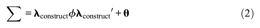
The customary one-factor CFA measurement model is usually a congeneric model (Brown, 2015; Graham, 2006). It includes one latent variable (= factor) representing the construct of interest, ξ_construct. The version for the application to centered data has the following structure:

x = λ_{construct} ξ_{construct} + δ

(1)

where x is the p×1 vector of centered manifest variables, λ_construct is the p×1 vector of factor loadings, ξ_construct is the latent variable, and $δ$ is the p×1 vector of residuals. Yet, important properties of the model-fit approach are not well represented by this model. Therefore, the measurement model is complemented by the corresponding p×p model-implied covariance matrix, Σ, expected to reproduce the p×p empirical covariance matrix, S (Gumedze & Dunne, 2011; Jöreskog, 1970). The structure of Σ is given by

\sum = λ_{construct} ϕ λ_{construct}' + θ

(2)

where λ_construct is the p×1 vector of factor loadings, λ_construct’ is the transposed version, ϕ is the variance parameter, and θ is the p×p diagonal matrix of residual variation. This model is expected to account for the systematic variation of data associated with the construct that is under investigation when parameters are appropriately specified. The first summand is thought to account for common systematic variation and the second one for unique systematic variation. θ is a diagonal matrix meaning that each off-diagonal entry, θ_ij (i, j = 1, . . ., p, i ≠ j), is zero, that is, reflects the principle of the model-fit approach mentioned in the introduction. As a consequence, the corresponding entry of the empirical covariance matrix, s_ij of S, is explained by σ_ij of Σ due to the contribution of the latent variable, ξ_construct, only:

s_{ij} \approx σ_{ij} = λ_{i} ϕ λ_{j}

(3)

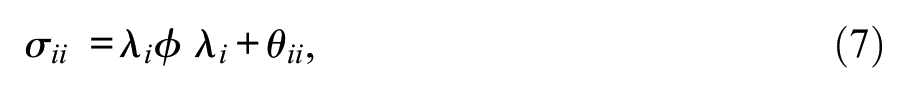
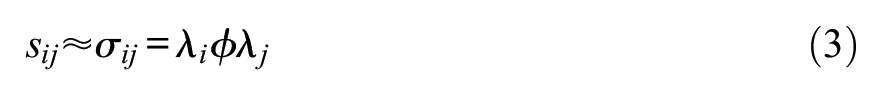
where ≈ signifies that σ_ij is assumed to closely correspond with s_ij because of approximation in estimation.

The Model With Correlated Residuals

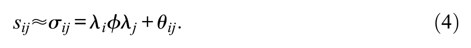
For considering a two-variable disturbance in the sense of correlated residuals, the described model-implied covariance matrix needs a modification. An off-diagonal entry of θ, θ_ij (i, j = 1, . . ., p, i ≠ j), has to be set free for estimation, while all other off-diagonal entries stay unchanged. Subscripts i and j identify the manifest variables assumed to show correlated residuals. This means that the covariance considered as disturbance, s_ij of S, is explained by σ_ij of Σ in the following way:

s_{ij} \approx σ_{ij} = λ_{i} ϕ λ_{j} + θ_{ij} .

(4)

Although setting free one entry of θ may be considered a minor modification, it is a clear violation of the original structure: what is actually part of common systematic variation and is normally represented by product λ_iϕλ_j is transformed into a mixture of common systematic variation (λ_iϕλ_j) and unique systematic variation (θ_ij).

Conceptualizing a two-variable disturbance this way does not only imply a violation of a basic principle. The possibility to investigate relationships of a factor representing additional systematic variation due to a two-variable disturbance with other factors or external variables is also omitted.

Models With a Method Factor

In contrast, treating a two-variable disturbance as an item-level method effect requires the transformation of the customary one-factor CFA measurement model into a two-factor CFA measurement model. Another latent variable (= factor) is integrated into the model for representing the item-level method effect. This modification turns the customary one-factor CFA measurement model into a bifactor CFA model (Reise, 2012) if at least one factor loading on one factor is not estimated but fixed. This requires the specification of one factor as factor representing the construct, ξ_construct, and the other factor as factor representing the method effect, ξ_ME. The resulting measurement model is

x = λ_{construct} ξ_{construct} + λ_{ME} ξ_{ME} + δ

(5)

where x is the p× 1 vector of centered manifest variables, λ_construct and λ_ME are the p× 1 vectors of factor loadings, ξ_construct and ξ_ME are the latent variables, and $δ$ is the p× 1 vector of residuals. The vectors of factor loadings differ in the following way: while ξ_construct receives factor loadings from all manifest variables, only the ith and jth manifest variables (i, j = 1, . . ., p) constituting the two-variable disturbance load on ξ_ME.

Because of the increase in the number of latent variables, the corresponding p×p model-implied covariance matrix, Σ (Equation 2), changes to

\sum = Λ Φ Λ' + θ

(6)

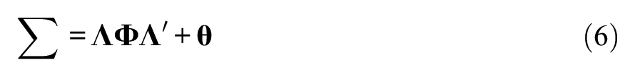
where Λ is the p× 2 matrix of factor loadings, Λ’ is the transposed version, Φ is the 2 × 2 matrix of variance and covariance parameters, and θ is the p×p diagonal matrix of residual variances. This model-implied covariance matrix is expected to account for the systematic variation of the p×p empirical covariance matrix, S.

For discussing the suitability of types of measurement models for representing two-variable disturbances, we treat the two-factor measurement model according to Equation 5 as a whole composed of two specific one-factor measurement models. We refer to them as construct submodel and method-effect submodel. Figure 1 illustrates how these submodels constitute the complete two-factor CFA measurement model for data with one item-level method effect.

Figure 1.

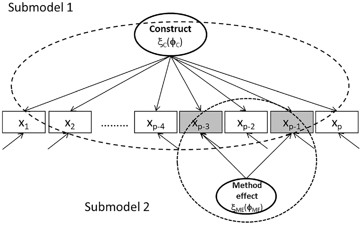
Illustration of Bifactor Model Including Latent Variables Representing Construct and Method Effect (Dashed-Line Ellipses Identify Construct Submodel 1 and Method-Effect Submodel 2).

The ellipse of the construct latent variable serves as starting point for arrows aiming at all rectangles representing p manifest variables. In contrast, only two arrows are rooted in the ellipse of the method latent variable and end up in two rectangles. Ellipses printed as dashed lines identify the two submodels.

Each submodel is expected to meet the requirements for measurement models. Especially, they are expected to allow for parameter identification. The customary one-factor CFA measurement model (Submodel 1) is a congeneric measurement model (Jöreskog, 1971) that is assumed to be just identified if there are three manifest variables and one parameter is fixed because of scaling. In the case of more manifest variables, it is assumed to be identified. This means that Submodel 1 is always at least just identified since it must include at least one more manifest variable than Submodel 2 that includes two of them.

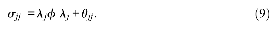
In the case of two manifest variables, the situation is as follows: starting from Equation 2 that fits with a measurement model including two manifest variables (ith and jth manifest variables taken from a larger set of manifest variables) like Submodel 2, there are three entries of Σ (σ_ii, σ_ij, σ_jj) (Note. σ_ji is omitted because it is identical with σ_ij) that approximate corresponding empirical information (s_ii, s_ji, s_jj) in parameter estimation. This means that according to Equation 2 there are the following three equations:

σ_{ii} = λ_{i} ϕ λ_{i} + θ_{ii},

(7)

σ_{ij} = λ_{i} ϕ λ_{j} + θ_{ij} with θ_{ij} = 0,

(8)

σ_{jj} = λ_{j} ϕ λ_{j} + θ_{jj} .

(9)

Parameter identification requires that this system of equations can be solved (= just identified) or, even better, that there is a surplus of empirical information (= identified), that is, the number of pieces of empirical information surmounts the number of parameters. Because of the need for scaling (Klopp & Klößner, 2020; Little et al., 2006; Schweizer et al., 2019), one parameter is usually fixed. For example, ϕ may be set equal to 1. This creates the following situation considering the congeneric model: there are only three pieces of empirical information, whereas the number of parameters that need to be estimated (λ_i, λ_j, θ_ii, θ_jj) is four. This means that this submodel is not identified.

The Tau-Equivalent Submodel

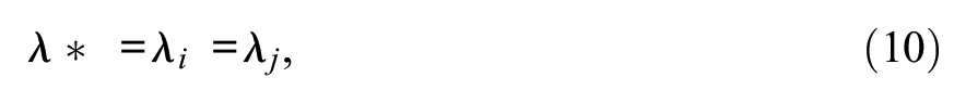
There are further types of measurement models besides the congeneric one that can alternatively be considered for serving as Submodel 2. First, there is the tau-equivalent model (Graham, 2006; Raykov, 1997). It is designed according to the true-score assumption of classical test theory (Lord & Novick, 1968, p. 47). According to this assumption, a participant’s response scores are composed of a true score and an error score, and the true score is the same for all items of a scale, whereas the error score may vary. Therefore, the tau-equivalent model of measurement constrains the sizes of factor loadings to the same value. This means that the tau-equivalent measurement model for two manifest variables includes the following constraints: (a) the factor loadings, λ_i and λ_j, on ξ_ME are set to equal sizes, λ*,

λ * = λ_{i} = λ_{j},

(10)

and (b) the variance parameter, ϕ_ME, of latent variable ξ_ME is fixed to one because of the need for scaling:

ϕ_{ME} = 1 .

(11)

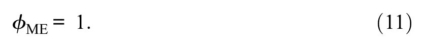
Fixing the variance parameter means scaling according to the reference group method; this implies that the information on explained variation is reflected by the factor loadings. Due to the constraints (Equations 10 and 11), the number of parameters that are to be estimated is three (λ*, θ_ii, θ_jj). This means that the tau-equivalent model is just identified (df_{tau-equivalent_submodel} = 0).

The Fixed-Links Submodel

Second, there is the fixed-links model (Schweizer, 2006, 2008) that was proposed for structural investigations on the basis of hypotheses regarding the relationships among items. The application of this model under the hypothesis of equal contributions of a latent source to two items creates similarity to the tau-equivalent measurement model. This model requires the assignment of the same positive numberic value to both factor loadings (λ_i and λ_j). If there is no reason for selecting a specific numberic value, the numberic value 1 is usually the default selected for constraining factor loadings:

1 = λ_{i} = λ_{j}

(12)

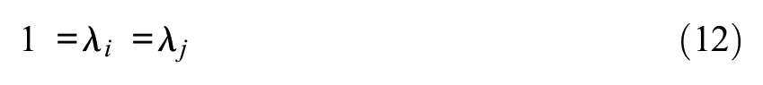
The fixing of factor loadings is compensated by estimating the variance parameter, ϕ_ME, which quantifies the latent variable, ξ_ME. In the case of this model, the number of the parameters to be estimated is also three (ϕ, θ_ii, θ_jj). Consequently, the fixed-links model is also just identified (df_{fixed-links_submodel} = 0).

The Parallel-Measurement Submodel

Third, there is the parallel-measurement model (Graham, 2006) that also has been discussed in the context of classical test theory (Lord & Novick, 1968, p. 58). The characteristic that distinguishes it from the tau-equivalent model is that equality of the residual variances is assumed in addition to equality of the factor loadings. Overall, this measurement model includes three constraints: the constraint of the factor loadings to equal sizes (Equation 10), the constraint of the variance parameter because of scaling (Equation 11), and the constraint of the residual variances (θ_ii and θ_jj) to equal sizes, θ*, which means

θ^{*} = θ_{ii} = {θ_{jj}}_{.}

(13)

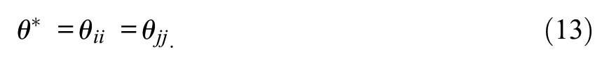
It needs to be mentioned that the parallel-measurement model as Submodel 2 implies impairment for Submodel 1 because of the constraint according to Equation 13. The freedom to estimate two residual variances of Submodel 1 independently is no more given. As only two parameters (λ*, θ*) need to be estimated in the parallel-measurement model, this model is considered identified (df_{parallel-measurement_submodel} = 1).

In sum, taking the perspective of model identification, there are three measurement submodels that can be employed for representing item-level method effects as part of a bifactor model without violating the basic principle regarding the subdivision of systematic variation. But, we are also aware that the congeneric submodel that is not considered can lead to a valid result in parameter estimation by EM algorithm.

A Simulation Study

The main objective of the empirical research was to compare the various ways of controlling a two-variable disturbance in investigating the structure of data by CFA. The various ways were realized as bifactor models including as one submodel the tau-equivalent measurement model, the fixed-links model, or the parallel-measurement model together with the customary one-factor CFA measurement model as the other submodel. In addition, the customary one-factor CFA measurement model adapted to correlated residuals was employed for investigating the data.

A one-dimensional underlying structure characterized the generated data besides a two-variable disturbance. The degree of disturbance was varied by manipulating the size of the covariance of the two variables. In addition, the environment of the disturbance, that is, the number of additional variables, was varied by modifying the number of manifest variables.

Method

Data giving rise to a two-variable disturbance were generated according to the method described by Jöreskog and Sörbom (2001), that is, continuous and normally distributed random data [N(0,1)] were generated and adapted to a given population pattern. The generation yielded sets of 500 500 × 5 and 500 500 × 10 matrices of structured random data based on population patterns differing according to the degree of disturbance. The number of rows was chosen to meet the recommendation for such investigations (Bader et al., 2021). The basic population pattern included coefficients of 0.20 as off-diagonal entries and 1.00 as diagonal entries so that the size of the factor loading expected under the assumption of one underlying dimension was 0.447. Further population patterns included a case of a two-variable disturbance characterizing a randomly selected pair of variables (the combination of the fourth column and eighth row in the larger data matrices and the combination of second column and fourth row in the smaller data matrices). The following sizes served as a two-variable disturbance: 0.35, 0.50, 0.65, and 0.80 in addition to 0.20 for no disturbance. They were referred to as increments of 0.15, 0.30, 0.45, 0.60 and 0.00 (= no increment) in corresponding order.

The following set of models served the statistical investigations of the generated data: (a) the customary one-factor CFA model with free factor loadings, (b) the one-factor CFA model with free factor loadings and correlated residuals, and also (c) three versions of the bifactor CFA model. The versions of the bifactor CFA model included a general factor with free factor loadings and a method-effect factor that was specified according to (c(i)) the tau-equivalent measurement model (Equations 10 and 11), (c(ii)) the fixed-links model (Equation 12), and (c(iii)) the parallel-measurement model (Equations 10, 11, and 13). The method-effect factor had loadings of either the second and fourth manifest variables or the fourth and eighth manifest variables depending on the number of columns of the data matrix.

The models, increments, and matrix sizes constituted a 5 × 5 × 2 design for the simulation study. The focus of the investigation was on model fit. It served checking whether the data manipulation creating disturbances led to impairment in model fit and whether measurement models for controlling such impairment were efficient in doing so.

Maximum Likelihood Estimation (MLE) was selected for parameter estimation by LISREL (Jöreskog & Sörbom, 2006). Covariances provided the input to CFA. If a data matrix did not prove to be positive definite, the ridge option was automatically performed (Yuan et al., 2011). The output of CFA was evaluated on the basis of root mean square error of approximation (RMSEA ≤ 0.6), standardized root mean squared residual (SRMR ≤ 0.8), non-normed fit index (NNFI ≥ 0.95), and comparative fit index (CFI ≥ 0.95) (DiStefano, 2016). Note. The numbers given in parentheses are cutoffs. χ² and Akaike information criterion (AIC) were additionally recorded.

Results

The results of investigating data matrices with five columns allowing for models with five manifest variables are included in Table 1.

Table 1.

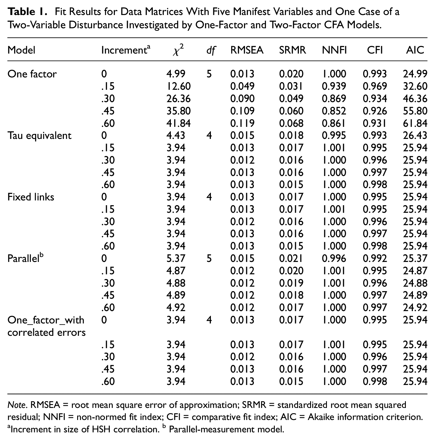
Fit Results for Data Matrices With Five Manifest Variables and One Case of a Two-Variable Disturbance Investigated by One-Factor and Two-Factor CFA Models.

Model	Increment^a	χ²	df	RMSEA	SRMR	NNFI	CFI	AIC
One factor	0	4.99	5	0.013	0.020	1.000	0.993	24.99
	.15	12.60		0.049	0.031	0.939	0.969	32.60
	.30	26.36		0.090	0.049	0.869	0.934	46.36
	.45	35.80		0.109	0.060	0.852	0.926	55.80
	.60	41.84		0.119	0.068	0.861	0.931	61.84
Tau equivalent	0	4.43	4	0.015	0.018	0.995	0.993	26.43
	.15	3.94		0.013	0.017	1.001	0.995	25.94
	.30	3.94		0.012	0.016	1.000	0.996	25.94
	.45	3.94		0.013	0.016	1.000	0.997	25.94
	.60	3.94		0.013	0.015	1.000	0.998	25.94
Fixed links	0	3.94	4	0.013	0.017	1.000	0.995	25.94
	.15	3.94		0.013	0.017	1.001	0.995	25.94
	.30	3.94		0.012	0.016	1.000	0.996	25.94
	.45	3.94		0.013	0.016	1.000	0.997	25.94
	.60	3.94		0.013	0.015	1.000	0.998	25.94
Parallel^b	0	5.37	5	0.015	0.021	0.996	0.992	25.37
	.15	4.87		0.012	0.020	1.001	0.995	24.87
	.30	4.88		0.012	0.019	1.001	0.996	24.88
	.45	4.89		0.012	0.018	1.000	0.997	24.89
	.60	4.92		0.012	0.017	1.000	0.997	24.92
One_factor_with correlated errors	0	3.94	4	0.013	0.017	1.000	0.995	25.94
	.15	3.94		0.013	0.017	1.001	0.995	25.94
	.30	3.94		0.012	0.016	1.000	0.996	25.94
	.45	3.94		0.013	0.016	1.000	0.997	25.94
	.60	3.94		0.013	0.015	1.000	0.998	25.94

Note. RMSEA = root mean square error of approximation; SRMR = standardized root mean squared residual; NNFI = non-normed fit index; CFI = comparative fit index; AIC = Akaike information criterion.

Increment in size of HSH correlation. ^b Parallel-measurement model.

Table 1 is organized according to the measurement models (first level) and the increment sizes (second level). The first to sixth rows include the results for the situation where the measurement model did not take the two-variable disturbance into consideration. Therefore, increasing the increment size was expected to be associated with a decreasing degree of model fit. This was true for RMSEA, SRMR, NNFI, and CFI. RMSEA, SRMR, NNFI, and CFI indicated good model fit in the absence of a disturbance (= zero increment, first row) and model misfit for the full disturbance (= largest increment, sixth row) except for SRMR and CFI. SRMR still signified good model fit, whereas CFI could be considered as acceptable model fit only. These results confirmed the expectation that the presence of a two-variable disturbance impairs model fit to a larger or lesser degree. The larger the increment, the larger the impairment.

All the other rows report results for models that take the two-variable disturbance into consideration. All results obtained by fit indices with a cutoff indicated good model fit. The degrees of variation across the increment sizes of many of them were small, as is obvious from the ranges of numbers included in the columns with results (χ²: 3.94–5.37, RMSEA: 0.012–0.015, SRMR: 0.015–0.021, NNFI: 0.995–1.001, CFI: 0.992–0.998, AIC: 24.87–26.43). The results obtained by the model including the fixed-links submodel and the model with correlated residuals exactly corresponded. This degree of correspondence did hold not only at the level of mean results but also at the level of individual investigations. There was also exact correspondence of these results in four out of the five increment levels with the results of the model including the tau-eq14 submodel. While the model, including the parallel-measurement submodel, yielded numerically slightly better RMSEA and AIC results, the SRMR and CFI results of other models were the numerically slightly better ones.

Next, the results of investigating data matrices with 10 columns allowing for 10 manifest variables are reported (see Table 2).

Table 2.

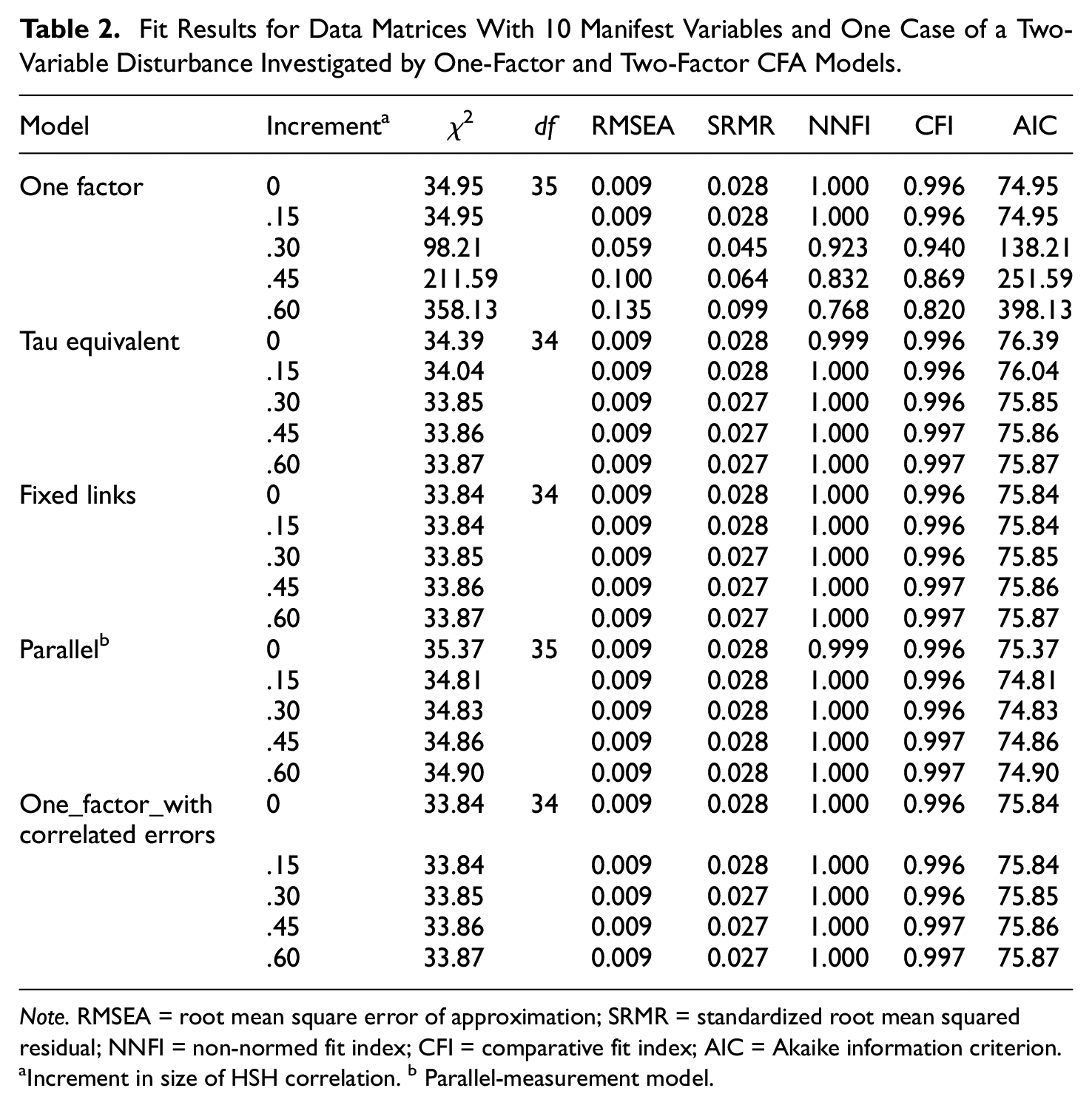
Fit Results for Data Matrices With 10 Manifest Variables and One Case of a Two-Variable Disturbance Investigated by One-Factor and Two-Factor CFA Models.

Model	Increment^a	χ²	df	RMSEA	SRMR	NNFI	CFI	AIC
One factor	0	34.95	35	0.009	0.028	1.000	0.996	74.95
	.15	34.95		0.009	0.028	1.000	0.996	74.95
	.30	98.21		0.059	0.045	0.923	0.940	138.21
	.45	211.59		0.100	0.064	0.832	0.869	251.59
	.60	358.13		0.135	0.099	0.768	0.820	398.13
Tau equivalent	0	34.39	34	0.009	0.028	0.999	0.996	76.39
	.15	34.04		0.009	0.028	1.000	0.996	76.04
	.30	33.85		0.009	0.027	1.000	0.996	75.85
	.45	33.86		0.009	0.027	1.000	0.997	75.86
	.60	33.87		0.009	0.027	1.000	0.997	75.87
Fixed links	0	33.84	34	0.009	0.028	1.000	0.996	75.84
	.15	33.84		0.009	0.028	1.000	0.996	75.84
	.30	33.85		0.009	0.027	1.000	0.996	75.85
	.45	33.86		0.009	0.027	1.000	0.997	75.86
	.60	33.87		0.009	0.027	1.000	0.997	75.87
Parallel^b	0	35.37	35	0.009	0.028	0.999	0.996	75.37
	.15	34.81		0.009	0.028	1.000	0.996	74.81
	.30	34.83		0.009	0.028	1.000	0.996	74.83
	.45	34.86		0.009	0.028	1.000	0.997	74.86
	.60	34.90		0.009	0.028	1.000	0.997	74.90
One_factor_with correlated errors	0	33.84	34	0.009	0.028	1.000	0.996	75.84
	.15	33.84		0.009	0.028	1.000	0.996	75.84
	.30	33.85		0.009	0.027	1.000	0.996	75.85
	.45	33.86		0.009	0.027	1.000	0.997	75.86
	.60	33.87		0.009	0.027	1.000	0.997	75.87

Note. RMSEA = root mean square error of approximation; SRMR = standardized root mean squared residual; NNFI = non-normed fit index; CFI = comparative fit index; AIC = Akaike information criterion.

Increment in size of HSH correlation. ^b Parallel-measurement model.

Table 2 is organized in the same way as Table 1 (the measurement models as first level and the increment sizes as second level). The results reported in the first to sixth rows were obtained without controlling disturbances due to increments. In this situation, decreasing degrees of model fit were expected for increasing increment sizes. RMSEA, SRMR, NNFI, and CFI results were in line with this expectation. In the absence of a two-variable disturbance (zero increment, first row), RMSEA, SRMR, NNFI, and CFI indicated good model fit, while in its presence (sixth row), three of them (RMSEA, NNFI and CFI) signified model misfit, whereas the SRMR result was not good but could be considered as still acceptable.

The fit result for the remaining models that did take the two-variable disturbance (see increment) into consideration was good and showed hardly any variation across the models or increment sizes (χ²: 33.84–35.37, RMSEA: 0.009–0.009, SRMR: 0.027–0.028, NNFI: 0.999 –1.000, CFI: 0.996–0.997, AIC: 74.81–76.39). Perfect correspondence of the fit results of the model including the fixed-links submodel and the model with correlated residuals was observed, as was in investigating data matrices with five columns (Table 1). The results for these models slightly differed from the results for the model including the tau-eq15 submodel in the first and second increment levels (0.00 and 0.15). In the remaining levels they also corresponded. While the model including the parallel-measurement submodel yielded numerically slightly better AIC results, the SRMR results of the other models were the numerically slightly better ones.

Figure 2 enables a comparison of the effects of disturbance sizes (increments) on model fit across smaller and larger sets of manifest variables.

Figure 2.

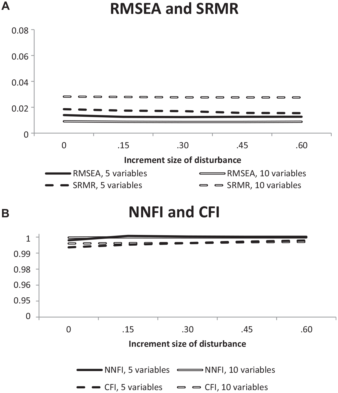
Diagrams Illustrating the Effect of Increasing the Increment Size on RMSEA and SRMR (A) as Well as on NNFI and CFI (B).

The curves were based on the means of the fit results for the measurement models taking a two-variable disturbance into consideration (tau-equivalent model, fixed-links model, parallel-measurement model, one-factor model with correlated residuals) since the focus was on the difference in the environment of a two-variable disturbance, that is, the number of additional variables (three or eight other manifest variables). Figure 2A includes the RMSEA and SRMR results as curves based on the investigation of 500 × 5 and 500 × 10 data matrices. All curves showed almost horizontal courses. Whereas the RMSEA curve showed a smaller overall level in 10-variable data than in five-variable data, the overall level of the SRMR curve was higher in 10-variable data than in five-variable data. Figure 2B includes the curves prepared from NNFI and CFI results. Horizontal courses characterized these curves when the number of manifest variables was 10. In contrast, there was a slight increase from no increment to an increment of 0.15 when the number of manifest variables was five. In larger increments, the curves also showed horizontal courses.

In sum, all models controlling the effect of a two-variable disturbance on the outcome of investigating the fit of the analysis model to the data signified good model fit while the neglect of controlling such disturbance led to model misfit. Increasing the degree of disturbance did not influence fit outcomes in any way in models adapted to such disturbance, while in the customary model without such a provision, the deviation from good model fit reflected the size of the increment.

Discussion

The conceptualization of a two-variable disturbance as either correlated residuals or an item-level method effect implies the decision for one of two different treatments of this disturbance in data analysis, although in both cases, the model-fit approach (Gumedze & Dunne, 2011; Jöreskog, 1970) provides the framework. Analyses checking the compatibility of the treatments with this approach reveal that only the conceptualization as item-level method effect fits, whereas the other conceptualization implies a violation of one of its basic principles. But, as it turns out, the practical consequences of switching between these conceptualizations are negligible. Starting from either conceptualization, the virtually same fit results are achieved.

Ignoring two-variable disturbances in structural investigations by CFA is likely to lead to model misfit because CFA is basically a method that checks for deviations from a more or less uniform correlation or covariance pattern (except of the main diagonal). Close correspondence with such a pattern can be achieved by selecting items for a scale so that their pairwise relationships are very similar. This means that it may not be sufficient to concentrate on item validity in scale construction (Markus & Borsboom, 2013) when it is the plan to demonstrate structural validity by CFA. Item subsets composed of items showing higher correlations among each other than the remaining items of the scale are likely to lead to failure in CFA. This is not only demonstrated by the results of the reported research (see results for the original one-factor CFA model) but is also in line with consequences of using items with identical meanings (Bandalos, 2021). Another possible result of ignoring two-variable disturbances is a possible bias in parameter estimation (Montoya & Edwards, 2021).

A new type of method effects is proposed for avoiding the violation of the basic principle of the model-fit approach. Like established method effects (scale-level method effects), item-level method effects refer to variation in measurement due to the measurement method (Maul, 2013; Schweizer, 2020; Sechrest et al., 2000). An item-level method effect is additional common systematic variation on top of common systematic variation extending to all items of the corresponding scale. Since common systematic variation due to the attribute is expected to extend to all items and the additional systematic variation characterizes a subset of all items only, it remains to refer to it as item-level method effect (if a very small error probability also characterizes the two-variable disturbance).

The possibility of additional common systematic variation is suggested by theory of personality. For example, there is the theory of social cognition/situation specificity of social learning asserting that people learn to respond to specific stimuli or situations in a unique way (Mischel, 2007). According to this theory, the more specific stimuli or situations are, the more likely people are to respond in the associated unique way after learning the association. Therefore, high specificity of items together with similar contents may lead to especially large correlations or covariances with consequences for consistency and reliability in assessment (Patry, 2011). This argument suggests that two-variable disturbances are not just random effects; instead they should be treated as item-level method effects. Distinguishing between disturbances deserving to be classified as item-specific method effects and other disturbances may require more research.

Given that the switch from correlated residuals to item-level method effects finds acceptance, the question for appropriate ways of representing such effects in CFA gains importance. This question leads to the bifactor model (Reise, 2012) including a one-factor measurement submodel for representing such an effect. Our analyses reveal that the tau-equivalent model, the parallel-measurement model, and the fixed-links model are suitable for this purpose. Negligible numerical differences regarding efficiency in securing good model fit distinguish the models. Only AIC signifies a small advantage for the parallel-measurement model as the most parsimonious model. Furthermore, astonishing degrees of similarity are revealed for the one-factor model with correlated residuals and the fixed-links model, and essentially also the tau-equivalent model.

To select a model for application, the assumptions characterizing the models can be consulted. The parallel-measurement model includes the largest number of restricting assumptions (Equations 10, 11, and 13) and, therefore, is the model that is most likely to fail in an application compared with the other models. The tau-equivalent model and the fixed-links model include the same number of assumptions and produced corresponding results except for the cases with no or only small two-variable disturbances. The advantage of the tau-equivalent model is that it produces conventional output, that is, factor loadings, whereas the advantage of the fixed-links model is the adaptability to situations where manifest variables show non-negligible differences in size. This information should facilitate selection.

The focus of the present article on the bifactor model including a submodel for representing a two-variable disturbance does not mean that the use of the bifactor model is restricted to such disturbances only. A disturbance may involve more than two manifest variables, as is, for example, the case in applications of tests that are composed of the so-called testlets (DeMars, 2006). Since in larger numbers of interrelated disturbance variables even the congeneric measurement model (Brown, 2015; Graham, 2006) can serve as a submodel, the resulting combination of submodels corresponds to the standard case of the bifactor model so that there is no need for further concerns.

Before closing the discussion, we would like to outline the additional advantages of conceptualizing correlated residuals as item-level method effects. First, there is the opportunity to clarify the contents associated with the systematic variation captured by the method factor by relating this factor to other factors of the model and to external variables. This means that it is possible to identify the kind of distortion of scores that can be expected if the corresponding two-variable disturbance is ignored. Second, it is possible to estimate the amount of variation that is explained by the method factor. The variances of the factors of a bifactor model can be estimated, given appropriate scaling (Schweizer & Troche, 2019), and the corresponding error probabilities can be determined. This may be helpful in deciding whether the amount of the disturbance is disadvantageous to the validity of measurement. Neither correlations with other factors and external variables nor information on the factor variances can be made available when computing correlated residuals.

While the use of correlated residuals is usually restricted to the structural investigation of data with no consequences for the application of a scale, the use of a method factor as part of a bifactor model enables using established factor-analytic techniques for decomposing systematic variation of data into components and for the computation of factor scores. Furthermore, there is the possibility to estimate the reliability of factor scores associated with the main factor as consistency by McDonald’s (1999) Omega.

A limitation of the present study is its concentration on the comparison of measurement models, while the question regarding the compatibility with the confirmatory nature of this approach is not addressed. Furthermore, the study does not provide advice on how to identify item-level method effects. In this case, resorting to explorative procedures may be helpful (Ferrando et al., 2022). Another limitation is that we did not investigate how controlling item-level method effects compares with the simple elimination of items.

Footnotes

Declaration of Conflicting Interests

The author(s) declared no potential conflicts of interest with respect to the research, authorship, and/or publication of this article.

Funding

The author(s) received no financial support for the research, authorship, and/or publication of this article.

ORCID iDs

Karl Schweizer

Dorothea Krampen

References

Bader

Jobst

L. J.

Moshagen

(2021). Sample size requirements for bifactor models. Structural Equation Modeling, 29(5), 772–782. https://doi.org/10.1080/10705511.2021.2019587

Bandalos

D. L.

(2021). Item meaning and order as causes of correlated residuals in confirmatory factor analysis. Structural Equation Modeling, 28(6), 903–913. https://doi.org/10.1080/10705511.2021.1916395

Brown

T. A.

(2015). Confirmatory factor analysis for applied research, (2nd ed.). The Guilford Press.

Byrne

B. M.

(2016). Using multitrait-multimethod analysis in testing for evidence of construct validity. In Schweizer

DiStefano

(Eds.), Principles and methods of test construction (pp. 288–307). Hogrefe.

Campbell

D. T.

Fiske

(1959). Convergent and discriminant validation by the multitrait-multimethod matrix. Psychological Bulletin, 56(2), 81–105. https://doi.org/10.1037/h0046016

DeMars

C. E.

(2006). Application of the bi-factor multidimensional item response theory model to testlet-based tests. Journal of Educational Measurement, 43(2), 145–168. https://doi.org/10.1111/j.1745-3984.2006.00010.x

DiStefano

(2016). Examining fit with structural equation models. In Schweizer

DiStefano

(Eds.), Principles and methods of test construction (pp. 166–193). Hogrefe.

Ferrando

P. J.

Fernandes-Dorad

Lorenzo-Seva

(2022). Detecting correlated residuals in exploratory factor analysis: New proposals and a comparison of procedures. Structural Equation Modeling, 29(4), 630–638. https://doi.org/10.1080/10705511.2021.2004543

Graham

J. M.

(2006). Congeneric and (essentially) tau-equivalent estimates of score reliability. Educational and Psychological Measurement, 66(6), 930–944. https://doi.org/10.1177/0013164406288165

10.

Gumedze

F. N.

Dunne

T. T.

(2011). Parameter estimation and inference in the linear mixed model. Linear Algebra and Its Application, 435(8), 1920–1944. https://doi.org/10.1016/j.Iaa.2011.04.015

11.

Jöreskog

K. G.

(1969). A general approach to confirmatory maximum likelihood factor analysis. Psychometrika, 34(2), 183–202. https://doi.org/10.1007/BF02289343

12.

Jöreskog

K. G.

(1970). A general method for analysis of covariance structure. Biometrika, 57(2), 239–251. https://doi.org/10.1093/biomet/57.2.239

13.

Jöreskog

K. G.

(1971). Statistical analysis of sets of congeneric tests. Psychometrika, 36(2), 109–133. https://doi.org/10.1007/BF02291393

14.

Jöreskog

K. G.

Sörbom

(2001). Interactive LISREL: User’s guide. Scientific Software International.

15.

Jöreskog

K. G.

Sörbom

(2006). LISREL 8.80: User’s reference guide. Scientific Software International.

16.

Klopp

Klößner

(2020). The impact of scaling methods on the properties and interpretation of parameter estimates in structural equation models with latent variables. Structural Equation Modeling, 28(2), 182–206. https://doi.org/10.1080/10705511.2020.1796673

17.

Landis

R. S.

Edwards

B. D.

Cortina

J. M.

(2009). On the practice of allowing correlated residuals among indicators in structural equation models. In Lance

C. E.

Vandenberg

R. J.

(Eds.), Statistical and methodological myths and urban legends: Verity and fable in the organizational and social sciences (pp. 193–214). Routledge/Taylor & Francis Group.

18.

Little

T. D.

Slegers

D. W.

Card

N. A.

(2006). A non-arbitrary method of identifying and scaling latent variables in SEM and MACS models. Structural Equation Modeling, 13(1), 59–72. https://doi.org/10.1207/s15328007sem1301_3

19.

Lord

F. M.

Novick

M. R.

(1968). Statistical theories of mental test scores. Addison-Wesley.

20.

Markus

K. A.

Borsboom

(2013). Frontiers of test validity theory: Measurement, causation, and meaning. Routledge.

21.

Maul

(2013). Method effects and the meaning of measurement. Frontiers in Psychology. https://doi.org/10.3389/fpsyg.2013.00169

22.

McDonald

R. P.

(1999). Test theory: A unified treatment. Lawrence Erlbaum.

23.

Mischel

(2007). Toward a science of the individual: Past, present, future? In Shoda

Cervone

Downey

(Eds.), Persons in context: Building a science of the individual (pp. 263–277). Guilford Press.

24.

Montoya

A. K.

Edwards

M. C.

(2021). The poor fit of model fit for selecting number of factors in exploratory factor analysis for scale evaluation. Educational and Psychological Measurement, 81(3), 413–440. https://doi.org/10.1177/0013164420942899

25.

Mulaik

S. A.

(2010). Foundations in factor analysis (2nd ed.). CRC Press.

26.

Patry

J.-L.

(2011). Methodological consequences of situation specificity: Biases in assessment. Frontiers in Psychology, 2, Article 18. https://doi.org/10.3389/fpsyg.2011.00018

27.

Raykov

(1997). Scale reliability, Cronbach’s coefficient alpha, and violations of essentially tau-equivalence with fixed congeneric components. Multivariate Behavioral Research, 32(4), 329–353. https://doi.org/10.1207/s15327906mbr3204_2

28.

Reise

S. P.

(2012). The rediscovery of bifactor measurement models. Multivariate Behavioral Research, 47(5), 667–696. https://doi.org/10.1080/00273171.2012.715555

29.

Schweizer

(2006). The fixed-links model in combination with the polynomial function as tool for investigating choice reaction time data. Structural Equation Modeling, 13(3), 403–419. https://doi.org/10.1207/s15328007sem1303_4

30.

Schweizer

(2008). Investigating experimental effects within the framework of structural equation modeling: An example with effects on both error scores and reaction times. Structural Equation Modeling, 15(2), 327–345. https://doi.org/10.1080/10705510801922621

31.

Schweizer

(2020). Method effects in psychological assessment. Psychological Test and Assessment Modeling, 64(3), 337–343.

32.

Schweizer

Troche

(2019). The EV scaling method for variances of latent variables. Methodology, 15(4), 175–184. https://doi.org/10.1027/1614-2241/a000179

33.

Schweizer

Troche

DiStefano

(2019). Scaling the variance of a latent variable while assuring constancy of the model. Frontiers in Psychology, 10, Article 887. https://doi.org/10.3389/fpsyg.2019.00887

34.

Sechrest

Davis

M. F.

Stickle

T. R.

McKnight

P. E.

(2000). Understanding‚ method variance. In Bickman

(Ed.), Research design: Donald Campbell’s legacy (pp. 63–87). SAGE.

35.

Thurstone

L. L.

(1947). Multiple-factor analysis. University of Chicago Press.

36.

Yuan

K.-H.

Bentler

P. M.

(2011). Ridge structural equation modeling with correlation matrices. British Journal of Mathematical and Statistical Psychology, 64(1), 107–133. https://doi.org/10.1348/000711010X497442

Conceptualizing Correlated Residuals as Item-Level Method Effects in Confirmatory Factor Analysis

Abstract

Keywords

Introduction

Measurement Models Taking Item-Level Method Effects Into Consideration

The Model With Correlated Residuals

Models With a Method Factor

The Tau-Equivalent Submodel

The Fixed-Links Submodel

The Parallel-Measurement Submodel

A Simulation Study

Method

Results

Discussion

Footnotes

Declaration of Conflicting Interests

Funding

ORCID iDs

References