Sage Journals: Discover world-class research

Abstract

Indirect indices for faking detection in questionnaires make use of a respondent’s deviant or unlikely response pattern over the course of the questionnaire to identify them as a faker. Compared with established direct faking indices (i.e., lying and social desirability scales), indirect indices have at least two advantages: First, they cannot be detected by the test taker. Second, their usage does not require changes to the questionnaire. In the last decades, several such indirect indices have been proposed. However, at present, the researcher’s choice between different indirect faking detection indices is guided by relatively little information, especially if conceptually different indices are to be used together. Thus, we examined and compared how well indices of a representative selection of 12 conceptionally different indirect indices perform and how well they perform individually and jointly compared with an established direct faking measure or validity scale. We found that, first, the score on the agreement factor of the Likert-type item response process tree model, the proportion of desirable scale endpoint responses, and the covariance index were the best-performing indirect indices. Second, using indirect indices in combination resulted in comparable and in some cases even better detection rates than when using direct faking measures. Third, some effective indirect indices were only minimally correlated with substantive scales and could therefore be used to partial faking variance from response sets without losing substance. We, therefore, encourage researchers to use indirect indices instead of direct faking measures when they aim to detect faking in their data.

Keywords

faking faking detection methods social desirability scale validity scale indirect indices

In the organizational context, self-report measures in a Likert-type-scale format are regularly used to assess different aspects of employees’ personality, leadership styles, attitudes, and more. However, the measures are valid only if respondents have answered the questions honestly. In high-stakes situations, such as job application settings, respondents may feel reluctant to be honest and instead answer the questionnaire items in a manner that they believe will best serve their personal goal (Goffin & Boyd, 2009; Holden & Book, 2012; Paulhus, 2002). It is therefore not surprising that faking detection research has gained considerable attention and that several methods for detecting faking have been proposed (Goffin & Christiansen, 2003; Holden et al., 2017; Lambert et al., 2016).

A common strategy to detect faking has been to add social desirability or validity scales to a questionnaire (see Goffin & Christiansen, 2003; Holden et al., 2017; Lambert et al., 2016). These scales commonly contain items about socially desirable behaviors and virtues that can only rarely be endorsed by honestly responding respondents (e.g., Paulhus, 2002). If a respondent nevertheless agrees with several of these socially desirable items, and thus achieves a high score on the corresponding scales, it is taken as an indication that the respondent is faking (e.g., Paulhus, 2002). However, the utility of these explicit or direct faking measures is questionable for several reasons. First, such overt items may be faked as well (Alliger et al., 1996; Kroger & Turnbull, 1975). Second, direct indices may not only measure the response style “faking” but may also capture variance components of the substantive measures (Connelly & Chang, 2016; Lanz et al., 2022). Third, the addition of such direct indices will lengthen the questionnaire, and lengthy questionnaires can be associated with increased test fatigue or even careless responding (Bowling et al., 2021). Together, this collectively underscores the need for careful consideration when implementing explicit faking measures and highlights the importance of addressing these potential drawbacks using different approaches.

A more reliable approach to assessing respondents’ faking might be the use of indirect or unobtrusive faking measures. These indices are calculated after survey completion and make use of a respondent’s deviant or unlikely response pattern over the course of a questionnaire to identify them as a faker. In the last decades, a wide variety of conceptually different indirect indices have been proposed for detecting faking. Based on previous reviews (e.g., Burns & Christiansen, 2011; Kiefer & Benit, 2016; Tracey, 2016), these indices can be categorized broadly as: (a) measures of response homogeneity, (b) measures reflecting a deviant response process, (c) measures of extreme responding, and (d) measures of inconsistency.

However, only few studies up to now have examined how these different types of indirect faking indices perform compared with each other. Moreover, the studies that have compared the performance of different indirect indices have been limited to one specific type of index (see Karabatsos, 2003, for a comprehensive comparison of several person-fit indices). Thus, at present, the researcher’s choice between different indirect faking detection measures is guided by relatively little information, especially if conceptually different indices are to be used together, such as the covariance index, the response latency index, the proportion of desirable scale endpoint responses, and the standardized log-likelihood.

This article has two major aims. For one, we want to examine how well conceptionally different indirect faking detection indices perform compared with each other. For another, we want to scrutinize how well the selected indirect indices perform (individually and jointly) compared with the current standard of faking detection—an established direct measure or validity scale. By examining these issues, we provide researchers with a differentiated basis upon which they can select and combine indirect indices for detecting faking in their data.

From the variety of indirect indices proposed in previous research (e.g., Burns & Christiansen, 2011; Kiefer & Benit, 2016; Tracey, 2016), we drew a representative selection of 12 indirect indices. The indirect indices were selected for the following reasons: First, we considered them as representative of one of the four broad screening principles (i.e., screening for response homogeneity, screening for a deviating response process, screening for extreme responding, and screening for response inconsistency) that we identified when studying the literature on detecting faking and other types of aberrant responding (e.g., careless responding, cheating). Second, they had already been successfully applied for detecting faking and other types of aberrant responding (e.g., careless responding, cheating).¹ Using indices that have primarily been used for careless responding or cheating detection (e.g., Mahalanobis distance, Guttman error index) together with established indirect faking indices (e.g., covariance index, response latency index) might therefore shed new light on the issue of faking detection and help to improve detection accuracy.

In the following, we first outline the fundamental concepts that underlie the selected 12 indirect indices. Subsequently, we elaborate on the research questions that stem from the identified research gap. In the final section, we then provide an overview of the three conducted studies aimed at addressing these research questions.

Measures of Response Homogeneity

Compared with honest responses on questionnaires, it is assumed that faked responses show increased homogeneity, because the respondents complete all questionnaire items with the same bias. In other words, in addition to the trait-specific influence of the substantive factors, all items are expected to be affected by the same common cause—the “ideal employee factor” (Burns & Christiansen, 2011). Two measures may be indicative of this increased homogeneity in faking response sets—the item-level covariance index (CVI; Burns & Christiansen, 2011; Christiansen et al., 2017) and intra-individual response variability (IRV; see Holden & Marjanovic, 2021). Compared with honest respondents, faking respondents should produce response sets in which the covariances among items are inflated and in which the variability of responses is reduced.

Measures That Reflect a Deviating Response Process

Faking respondents are also assumed to show a deviating or altered response process compared with honest respondents because they answer the items not as they apply to them but rather in accordance with their personal goal or schema. Thus, additional cognitive processes may be involved when respondents fake item responses. Two measures may reflect this deviating response process—response latencies (Holden et al., 1992) and the average number of clicks for selected items.

According to Holden et al. (1992, p. 273), schema-inconsistent responses should take longer than schema-consistent responses. Thus, if a respondent has adopted a faking-good schema, they should respond more slowly than honest respondents when rejecting a positive statement (Latency_reject). However, if a respondent has adopted a faking-bad schema, they should respond more slowly than honest respondents when endorsing a positive statement (Latency_endorse).

Based on Holden et al.’s (1992) hypothesis, we suspect that faking respondents are also more likely to correct their response in advance of submitting a schema-inconsistent response. This externalized thinking process should be reflected in more clicks per item until the final response is submitted. Thus, if respondents have adopted a faking-good schema, they should click more often until the final item response is submitted than honest respondents do when rejecting a positive statement (Clicks_reject). However, if respondents have adopted a faking-bad schema, they should click more often until the final item response is submitted than honest respondents do when endorsing a positive statement (Clicks_endorse).

Measures of Extreme Responding

To improve their chances of obtaining their personal goal, faking respondents are also expected to strongly agree with desirable items and to strongly disagree with undesirable items and thus to exhibit a more extreme response pattern than honest respondents (Landers et al., 2011; Levashina et al., 2014). Indices that make use of this more extreme response pattern to identify faking participants can be subsumed under the category “measures of extreme responding”. Examples of this index type are the proportion of desirable scale endpoint responses (e.g., Landers et al., 2011; Levashina et al., 2014), the factor scores of a Likert-type item response process tree model (LIRP-TM; Böckenholt, 2012, 2017; Sun et al., 2021), and the item–order correlation coefficient (Holden et al., 2017).

The proportion of desirable scale endpoint responses is probably the most intuitive measure when assessing the extremity of a response pattern. For this measure, simply, the number of desirable scale endpoint responses is counted and divided by the number of scale items. Three types of scale endpoint endorsement measures can be calculated—a first one that reflects the proportion of endpoint responses in favorable items for respondents that are faking good (Ppropex), a second one that reflects the proportion of endpoint responses in favorable items for respondents that are faking bad (Npropex), and a third one that reflects the mere proportion of endpoint responses in all substantive items (IDpropex; Borgatta & Glass, 1961, p. 215; König et al., 2015, p. 431). Because of the specific counting principle of extreme responses, Ppropex and Npropex are also referred to in the later sections of this paper as tailored scale endpoint endorsement measures. Generally, faking respondents are expected to have larger values on these indices than honest respondents (see Levashina et al., 2014).

In the LIRP-TM, in contrast, the extremity in the response pattern of faking respondents is captured by different response factors (i.e., midpoint [LIRP-TM-M], agreement [LIRP-TM-A], extremity [LIRP-TM-E]) and their scores (Böckenholt, 2012, 2017; Sun et al., 2021). For example, faking respondents are expected to have higher scores on the extremity factor than honest respondents (see Sun et al., 2021).

Finally, Holden et al. (2017) recently proposed that extremity in the response pattern of faking respondents can also be detected through the item–order correlation, which is the within-person correlation between the vector of item responses (in which all items need to be scored in the same direction [e.g., positivity]) and that of the item order. Hence, respondents with a faking good schema should have higher correlation coefficients than honest respondents, and respondents with a faking bad schema should have lower correlation coefficients than honest respondents (see Holden et al., 2017).

Measures of Inconsistency

If faking respondents respond in a homogeneous fashion or only choose extreme response options across many items, this will eventually result in an overall response pattern that has a low probability of occurrence. In other words, it is likely that faking respondents produce a response pattern that is inconsistent in two ways. For one, their response pattern is expected to be inconsistent with the normative response pattern (the sample norm of honest respondents). The Mahalanobis distance (Mahalanobis, 1936) and the person-total/personal-biserial correlation coefficient (r_pbis; Donlon & Fischer, 1968) reflect this type of inconsistency. For another, their response pattern is expected to be inconsistent with the expected model parameters (their response pattern fits the estimated measurement model poorly). The normed Guttman error index for polytomous items (Gnormed; Emons, 2008), the standardized log-likelihood for polytomous items (lz; Drasgow et al., 1985), and the individual contribution to the model misfit or χ² (INDCHI; Reise & Widaman, 1999) are examples of indices that reflect this model-based inconsistency.

Inconsistency With the Sample Norm

Typically, the Mahalanobis distance has been used in regression analyses for detecting multivariate outliers (see Tabachnick & Fidell, 2007, pp. 73–77). In this context, a large distance value indicated that a respondent’s response pattern deviated significantly from the sample centroid, and thus could be treated as a potential outlier. Recently, however, the Mahalanobis distance has also been used for detecting careless responding (Goldammer et al., 2020). Thus, if this distance measure can detect one type of aberrant responding (i.e., careless responding), it may also be useful in detecting other types, such as faking. If our proposition is true, response protocols of faking respondents (like those of careless respondents) should be indicated by large distance values and those of honest respondents (like those of careful respondents) by small distance values.²

The r_pbis works like an item–total or item–rest correlation in the context of a scale reliability analysis (Curran, 2016, pp. 12–13). Like an item that should correlate positively with the rest of the scale items, the response patterns of individual respondents should correlate positively with the response pattern of the sample norm. In both cases, low or even negative correlation coefficients are a point of concern, as they indicate inconsistency. As this index turned out to be effective in detecting other forms of aberrant responding (e.g., careless, random, or cheating; see Karabatsos, 2003), we expect this index to be also effective in detecting faking. If this proposition is true, faking respondents should have lower item–total correlation coefficients than honest respondents, just as careless respondents should have lower item–total correlation coefficients than careful respondents (see Footnote 2).

Inconsistency With Expected Model Parameters

The basic idea of Guttman errors is that respondents are expected to answer test items in accordance with their total score (e.g., Meijer et al., 2016; Niessen et al., 2016). In the context of polytomous items, a respondent has produced a Guttman error if they have taken an unpopular item step after they have not taken a more popular item step in advance (Niessen et al., 2016, pp. 10–11). Because the Gnormed has been successfully applied to detect careless responding (Niessen et al., 2016), it is likely that this index is also effective in detecting faking. Accordingly, faking respondents should have larger Gnormed values than honest respondents, just as careless respondents should have larger Gnormed values than careful respondents (see Footnote 2).

The lz follows a very similar logic. Generally, participants are expected to respond to items according to their latent trait level. Inconsistently responding respondents, however, provide a response pattern that is very unlikely under the person’s latent trait level. This deviation is captured by the lz (Niessen et al., 2016, p. 4), and the misfit of a person’s response pattern is indicated by large negative values (Reise & Widaman, 1999, p. 6). Thus, faking respondents are expected to have lower lz values than honest respondents, just as careless respondents are expected to have lower lz values than careful respondents (see Footnote 2).

In the case of the INDCHI, in contrast, the inconsistency of a respondent’s response pattern is determined through the comparison of two covariance structure models—the saturated model and the substantive factor model (Reise & Widaman, 1999). This results in a statistic, INDCHI, that reflects the individual contribution to the overall model misfit (Reise & Widaman, 1999). Respondents with a response pattern that is rather unlikely under the estimated factor model will have larger INDCHI values than respondents that have produced a response pattern that is consistent with the estimated factor model (Reise & Widaman, 1999). Accordingly, we expect faking participants to have larger INDCHI values than honest respondents, just as careless respondents are expected to have larger INDCHI values than careful respondents (see Footnote 2).

Indirect Faking Measures: Unknowns

As the review of the 12 indices shows, there are several promising indirect indices available if faking needs to be detected in data sets. However, researchers still face several unanswered questions if they want to apply one or several of these indirect indices. First, even though researchers may be interested in only one particular indirect index, they will quickly realize that different calculation methods (subversions) are available and that only little is known about which of these calculation methods perform best in detecting faking respondents. For instance, for indices like the lz or the proportion of desirable scale endpoint responses, a scale-specific and global version (i.e., the average of scale-specific indices) can be calculated. Taking the perspective of a reliability analysis, including more items in the calculation may result in a more reliable or accurate faking index. However, it may be also argued that “desirable variance” is not equally distributed across personality traits and the corresponding items (Holden et al., 2017, p. 198). In other words, some traits/items may be considered as more goal-relevant than others and thus will more likely be faked. Accordingly, a scale-specific version of such an index may be better at detecting faking respondents than the global version of this index.

If a normative sample is at hand, researchers also have the choice between subversions when calculating the Mahalanobis distance and the r_pbis. Should the distance/correlation be computed at once for the total sample, or should the calculation take place in subsamples (i.e., to separately merge each participant of the test sample with the normative sample)? Thus, the following research question should be addressed.

Research Question 1 (RQ1): When subversions can be computed for an index, which of these is the most accurate faking detection measure?

If a researcher wishes to use multiple indirect indices to detect faking, there is not only the question of the calculation method for each index but also the question of which of the various available indirect indices to use. Unfortunately, the researcher’s choice between different indirect faking detection measures is guided by relatively little information so far, especially if conceptually different indices are to be used together, such as the CVI, the response latency index, the proportion of desirable scale endpoint responses, or the lz. We therefore addressed the following research question:

Research Question 2 (RQ2): How accurately do the 12 indirect indices detect faking compared with each other?

In addition, many of the 12 indices (i.e., IRV, clicks per item, the proportion of desirable scale endpoint responses; factor scores of the LIRP-TM, Mahalanobis distance, r_pbis, Gnormed, INDCHI) have not yet been compared with the current standards of faking detection—an established direct measure or validity scale such as the Balanced Inventory of Desirable Responding (BIDR; Paulhus, 1994). We therefore also addressed the following research question:

Research Question 3 (RQ3): How accurately do these 12 indirect indices detect faking compared with a direct faking measure?

If several of these indices turn out to be effective in detecting faking and increase the classification accuracy beyond a direct faking measure, it would be also interesting to see whether a selected group of indirect indices as set can even outperform a direct faking measure. The following research question was therefore also addressed:

Research Question 4 (RQ4): How accurately does a set of effective indirect indices detect faking compared with a direct measure?

To examine the four research questions, we conducted three studies. In Study 1 and Study 2, we examined the indices’ detection accuracy based on experimentally induced faking response sets. In Study 3, to assess the robustness of the indices’ performance in an applied setting, we investigated their detection accuracy in the context of naturally occurring faking. However, a reviewer criticized the length of the earlier version of the manuscript and considered Studies 2 and 3 as superfluous regarding the main purposes of the manuscript. We therefore decided to report the method and results of Study 2 and 3 only as Supplementary Material.

Method

Besides providing initial insights regarding our research questions, in this study, we examined whether the indirect indices have a different utility for detecting different forms of faking (i.e., faking good and faking bad). As previous studies suggest, respondents that are faking bad may produce more obvious response patterns than those who are faking good (e.g., Röhner et al., 2011, 2022). It therefore seems plausible that the examined faking indices perform better when the aim is to detect faking bad instead of faking good (e.g., Röhner et al., 2011, 2022).

Procedure and Participants

The participants were 320 German-speaking conscripts doing their military service in the summer of 2020 in two randomly drawn basic military training camps. After the data gathering, the data protocols of the 320 participants were examined for careless responding. This included screening the average response time per item for implausible fast responding (i.e., faster than the rate of 2 s per item; Huang et al., 2012, p. 106), screening for duplicate response protocols, and screening for participants with missing values for more than half of the questionnaire items. However, none of the participants was identified as careless responder according to these criteria. All 320 participants were therefore included in the following analyses.

The participants in this sample were on average 20.20 years old (SD = 1.19) and predominantly men (n = 318, 99.4%). The educational level of the participants in the study was as follows: Almost a third (n = 105, 32.8%) had completed upper secondary school, and the majority (n = 201, 62.8%) had completed a certified apprenticeship. Only a minority of the participants (n = 14, 4.4%) had completed only the 9 years of compulsory schooling.

Experimental Conditions and Survey Arrangement

The data were gathered platoon-wise. After providing the participants with a general introduction, we randomly assigned them to one of three experimental conditions—to the honest responding condition (n = 105) or to one of the two faking responding conditions (i.e., Fake-Good [n = 107], Fake-Bad [n = 108]). Civilian instructors, who were randomly assigned to one of the three conditions, then led the three subgroups into separate labs. All participants were then told that they would now take part in an experiment that was about how to best identify faking in survey data and that all participants would receive 10 Swiss francs as compensation for their efforts after completion of the survey. All participants were asked to imagine that the results of the questionnaire would be used to select future cadres of the Swiss Armed Forces. Participants in the honest responding group were then asked to complete the questionnaire accurately and honestly; participants in the faking responding conditions were asked to fake the questionnaire to achieve their goal (i.e., being perceived as either fit or unfit for a cadre position), without being caught out by our faking detection measures. After this instruction, the participants began completing the online questionnaire. After they had answered three sociodemographic questions, they completed the main part of the questionnaire, in which the order of the items was randomized and each item was displayed on a single web page.

Substantive Measures

Two substantive measures were included in the questionnaire—a personality inventory and a scale to measure affective motivation to lead (MTL). The personality inventory was the German translation of the 60-item version of the HEXACO (Ashton & Lee, 2009), which measures the six trait scales honesty-humility (α_Honest = .70, α_Fake-Good = .63, α_Fake-Bad = .69), emotionality (α_Honest = .80, α_Fake-Good = .72, α_Fake-Bad = .73), extraversion (α_Honest = .82, α_Fake-Good = .78, α_Fake-Bad = .79), agreeableness (α_Honest = .76, α_Fake-Good = .64, α_Fake-Bad = .75), conscientiousness (α_Honest = .82, α_Fake-Good = .81, α_Fake-Bad = .85), and openness (α_Honest = .79, α_Fake-Good = .63, α_Fake-Bad = .70). To measure the participants’ affective MTL, we used the nine items of the German adaption (Felfe et al., 2012) of Chan and Drasgow’s (2001) affective MTL subscale (α_Honest = .90, α_Fake-Good = .74, α_Fake-Bad = .78). In contrast to the HEXACO and MTL manuals, which specify a 5-point scale as response format, all items of these measures were rated on a Likert-type scale ranging from 1 = completely disagree to 6 = completely agree to avoid mid-point responses.

Direct Faking Measure

As a measure of direct faking we used the German impression management (IM) scale by Musch et al. (2002), which is based on the IM subscale of the BIDR, Version 6 (Paulhus, 1994). This measure was chosen because we considered the IM as a timely and popular faking measure that could be readily applied in our study. In contrast to the IM manual, which specifies a 7-point scale as response format, the 10 items of this measure were rated on a Likert-type scale that ranged from 1 = completely disagree to 6 = completely agree to avoid mid-point responses. For the main analyses, an average score was computed across the 10 items (α_Honest = .71, α_Fake-Good = .78, α_Fake-Bad = .80). If a respondent’s response was missing, the IM average score was based on the remaining non-missing responses.

Indirect Faking Measures

We calculated the 12 indirect indices from our representative selection and for 10 of them, additional subversions that were based on different calculation methods. For computing these indirect indices and subversions, only the 69 items of the seven substantive scales were used. Detailed information on how these indices were computed is provided in the Supplemental Material.

Faking Criterion and Analytical Procedure

The indices’ classification accuracy of fakers and non-fakers was our outcome variable. We therefore plotted for every index (and selected combinations of indices) a receiver operating characteristic (ROC) curve (e.g., Swets, 1986) and examined the corresponding area under the curve (AUC). We used the nonparametric method for plotting the ROC curves and for estimating the AUCs, and we used the method proposed by DeLong et al. (1988) for calculating the standard errors for each AUC and the differences between AUCs. All these analyses were performed in Stata (StataCorp, 2021).

Results

Manipulation Check

Compared with the honest responding group, the respondents in the Fake-Good condition had higher scale scores for “desirable” traits (e.g., Honesty-Humility, Extraversion, Conscientiousness, Motivation to lead) and a lower scale score for the “undesirable” trait emotionality (see Table 1). The expected mean shift could also be observed in the Fake-Bad condition. In addition, the averaged inter-scale covariance for faking respondents tended to be inflated (see Table 1), even though the global equality test of the averaged scale covariances did not reach the Bonferroni-corrected alpha level. Based on these results, we concluded that the response set manipulation was successful and that the effect of the manipulation on the substantive scales was strong (d, see Table 1).

Table 1

Comparison of Substantive Scale Scores and Their Interrelatedness Across Conditions

	Response conditions
	Honest	Fake-Good	Fake-Bad
Measures	M (SD)	M (SD)	M (SD)	χ₂(2)	Cohen’s d
Scale
Honesty-Humility	4.01_a (0.73)	4.39_b (0.74)	2.82_c (0.81)	235.48*	0.51_FG/–1.53_FB
Emotionality	3.08_a (0.75)	2.38_b (0.70)	4.21_c (0.86)	294.52*	−0.95_FG/1.40_FB
Extraversion	4.04_a (0.74)	5.12_b (0.62)	2.66_c (0.85)	603.49*	1.58_FG/–1.73_FB
Agreeableness	3.96_a (0.69)	4.11_a (0.69)	2.77_b (0.82)	192.15*	0.22_FG/–1.56_FB
Conscientiousness	4.02_a (0.75)	5.20_b (0.62)	2.33_c (0.84)	821.40*	1.70_FG/–2.13_FB
Openness	3.40_a (0.88)	3.86_b (0.72)	3.07_a (0.88)	53.42*	0.56_FG/–0.38_FB
Motivation to lead (affective)	3.39_a (0.97)	4.96_b (0.80)	2.29_c (0.83)	593.20*	1.77_FG/–1.23_FB
Inter-scale relatedness
Covariances_#	0.14 (0.11)	0.19 (0.08)	0.31 (0.10)	8.75

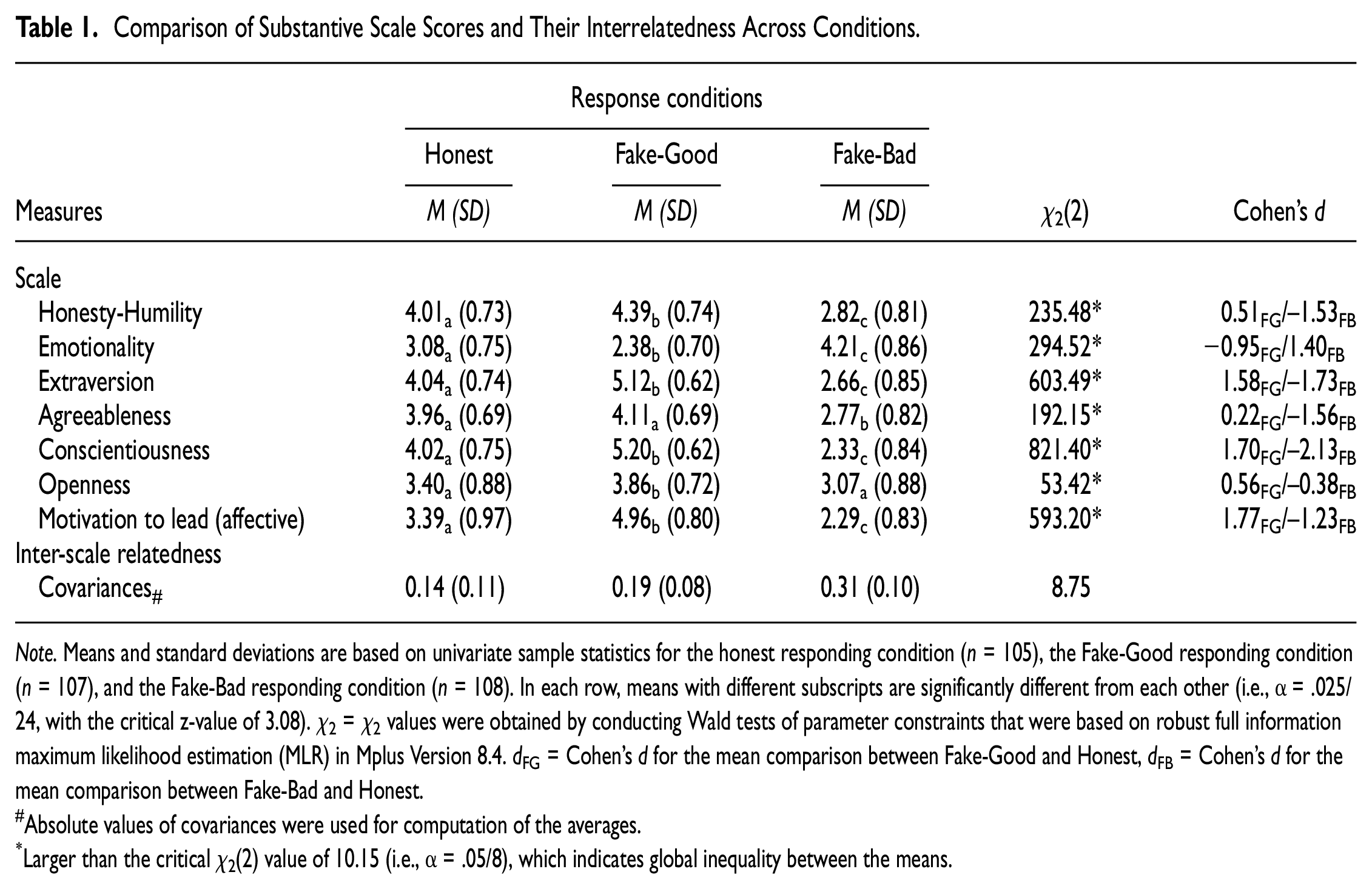
Note. Means and standard deviations are based on univariate sample statistics for the honest responding condition (n = 105), the Fake-Good responding condition (n = 107), and the Fake-Bad responding condition (n = 108). In each row, means with different subscripts are significantly different from each other (i.e., α = .025/24, with the critical z-value of 3.08). χ₂ = χ₂ values were obtained by conducting Wald tests of parameter constraints that were based on robust full information maximum likelihood estimation (MLR) in Mplus Version 8.4. d_FG = Cohen’s d for the mean comparison between Fake-Good and Honest, d_FB = Cohen’s d for the mean comparison between Fake-Bad and Honest.

Absolute values of covariances were used for computation of the averages.

Larger than the critical χ₂(2) value of 10.15 (i.e., α = .05/8), which indicates global inequality between the means.

Descriptive Statistics

The condition-specific correlation matrices as well as the condition-specific means and standard deviations of the substantive measures and faking indices are reported in the Supplemental Material (see Tables S1–S3).

Within-Index Comparisons Between Different Calculation Methods

The results of these within-index comparisons are displayed in Supplemental Material Table S4. In the vast majority, global versions of indices performed better than scale-specific versions (e.g., Gnormed, lz, INDCHI). Only if MTL was used for calculation, some scale-specific indices outperformed their global counterpart (e.g., LIRP-TM-E, IDpropex). For further analyses, we therefore used only global versions of indices (indicated by the subscript _global).

For indices that involved an explicit comparison with the sample norm (i.e., Mahal, r_pbis, INDCHI), calculations based on subsamples resulted in more accurate indices than calculations in which the indices were obtained at once in the total sample. Therefore, only subsample-based calculations of these indices were used for further analyses (indicated by the subscript _avr).

In the case of IRV, the results were unexpected in two respects. First, the IRV that was based on unidirectionally positively scored items (i.e., IRV_scored; Holden & Marjanovic, 2021, p. 3) turned out to be ineffective. Second, the alternative IRV measure that was based on raw item scores (see Goldammer et al., 2020) turned out to screen in the wrong direction. Contrary to what we had thought and in line with Holden and Marjanovic’s (2021) expectation, larger IRV values were more indicative of faking good and bad. Therefore, only the raw scores-based IRV (IRV_raw) with adjusted screening direction was used for further analyses.

Of the three types of scale endpoint endorsement measures (Ppropex, Npropex, IDpropex), the tailored measures (i.e., Ppropex, Npropex) turned out to be more accurate than the measure in which all endpoint responses were counted irrespective of the respondent’s faking schema (i.e., IDpropex). Therefore, only Ppropex and Npropex were used for further analyses.

Finally, we also compared the three response factor scores in the LIRP-TM regarding their detection accuracy, and the score on the agreement factor (i.e., LIRP-TM-A) was the only one that could detect both forms of faking with a high level of accuracy. Therefore, only the LIRP-TM-A was used for the further analyses.

Comparisons Between the Indirect Indices

For detecting respondents that were faking good, LIRP-TM-A_global, Ppropex_global, IRV_raw, and CVI outperformed almost all other indices (see Table 2). Compared with these four indices, Gnormed_global, lz_global, r_pbis.avr, Latency_reject, Mahal_avr and Clicks_reject were not as accurate, but they still performed better than chance. In contrast, the INDCHI_global.avr and item–order correlation did not perform well in detecting respondents that were faking good. The accuracy of these indices was not better than chance.

Table 2

Ordered Accuracies of the 12 Indirect Indices in Detecting Faking Good and Corresponding Pairwise Comparison Results

Index	AUC_{[95% CI]}	Sen95 ^a	Sen99 ^b	1.	2.	3.	4.	5.	6.	7.	8.	9.	10.	11.
1. LIRP-TM-A_global	.86_{[.81, .92]}	.57	.34
2. Ppropex_global	.85_{[.80, .90]}	.50	.43	0.12
3. IRV_raw	.84_{[.78, .89]}	.50	.39	0.67	1.56
4. CVI	.83_{[.77, .89]}	.42	.22	1.60	0.56	0.04
5. Gnormed_global	.73_{[.66, .80]}	.36	.14	7.96	18.43	18.33	4.77
6. lz_global	.66_{[.59, .74]}	.17	.09	15.09	32.30	28.72	10.93	11.88
7. r_pbis·avr	.64_{[.56, .71]}	.06	.03	18.99	20.48	18.13	14.04	4.57	0.37
8. Latency_reject	.62_{[.55, .70]}	.19	.17	36.57	27.00	22.47	21.94	3.99	0.53	0.06
9. Mahal_avr	.61_{[.53, .68]}	.11	.05	22.68	39.67	39.95	18.57	22.92	4.11	0.46	0.06
10. Clicks_reject	.58_{[.50, .66]}	.08	.02	37.81	40.68	34.27	27.09	10.79	3.21	1.11	0.67	0.30
11. INDCHI_global.avr	.58_{[.4985, .65]}	.18	.04	31.26	40.40	37.17	23.96	13.23	4.25	1.48	0.69	0.44	0.00
12. Item–order	.49_{[.41, .57]}	.08	.02	66.00	65.61	61.09	52.09	23.32	10.76	6.87	7.33	4.77	2.51	2.42

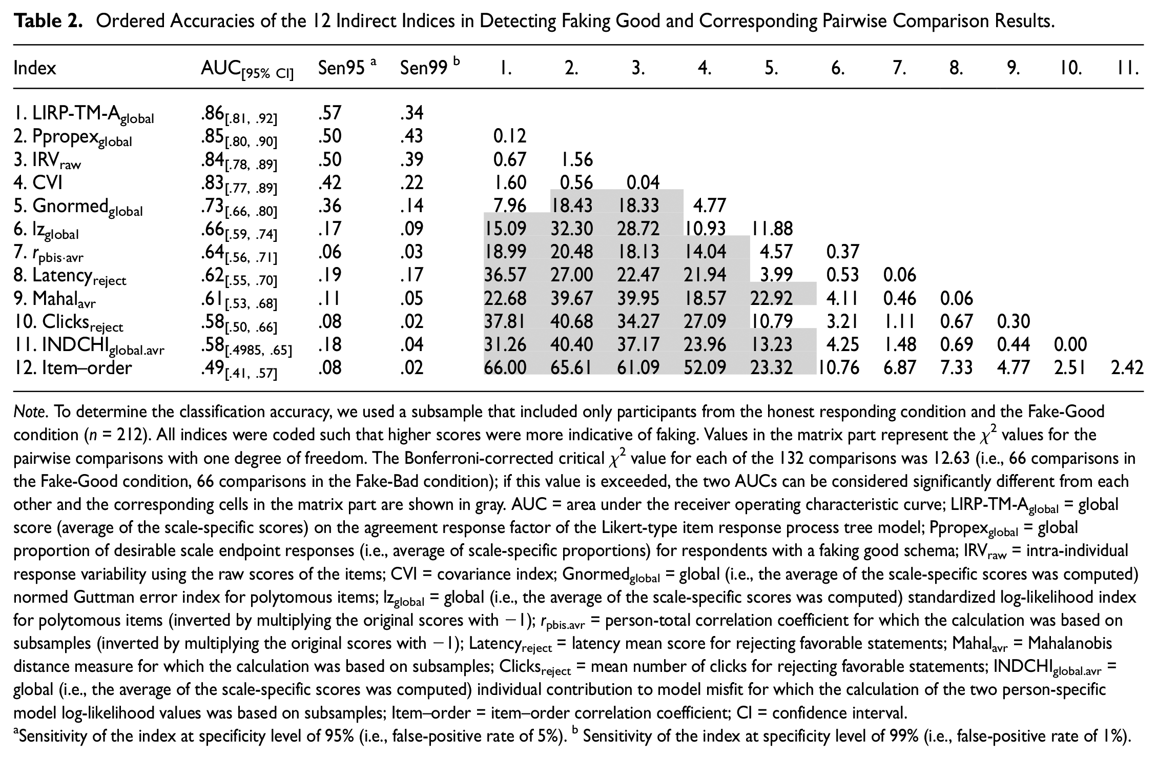
Note. To determine the classification accuracy, we used a subsample that included only participants from the honest responding condition and the Fake-Good condition (n = 212). All indices were coded such that higher scores were more indicative of faking. Values in the matrix part represent the χ² values for the pairwise comparisons with one degree of freedom. The Bonferroni-corrected critical χ² value for each of the 132 comparisons was 12.63 (i.e., 66 comparisons in the Fake-Good condition, 66 comparisons in the Fake-Bad condition); if this value is exceeded, the two AUCs can be considered significantly different from each other and the corresponding cells in the matrix part are shown in gray. AUC = area under the receiver operating characteristic curve; LIRP-TM-A_global = global score (average of the scale-specific scores) on the agreement response factor of the Likert-type item response process tree model; Ppropex_global = global proportion of desirable scale endpoint responses (i.e., average of scale-specific proportions) for respondents with a faking good schema; IRV_raw = intra-individual response variability using the raw scores of the items; CVI = covariance index; Gnormed_global = global (i.e., the average of the scale-specific scores was computed) normed Guttman error index for polytomous items; lz_global = global (i.e., the average of the scale-specific scores was computed) standardized log-likelihood index for polytomous items (inverted by multiplying the original scores with −1); r_pbis.avr = person-total correlation coefficient for which the calculation was based on subsamples (inverted by multiplying the original scores with −1); Latency_reject = latency mean score for rejecting favorable statements; Mahal_avr = Mahalanobis distance measure for which the calculation was based on subsamples; Clicks_reject = mean number of clicks for rejecting favorable statements; INDCHI_global.avr = global (i.e., the average of the scale-specific scores was computed) individual contribution to model misfit for which the calculation of the two person-specific model log-likelihood values was based on subsamples; Item–order = item–order correlation coefficient; CI = confidence interval.

Sensitivity of the index at specificity level of 95% (i.e., false-positive rate of 5%). ^b Sensitivity of the index at specificity level of 99% (i.e., false-positive rate of 1%).

For detecting respondents that were faking bad, r_pbis.avr and LIRP-TM-A_global outperformed all other indices (see Table 3). Compared with these two indices, Npropex_global, CVI, Mahal_avr, Gnormed_global, INDCHI_global.avr, lz_global, IRV_raw, and Latency_endorse were not as accurate, but they still performed better than chance. In contrast, the Clicks_endorse and item–order correlation did not perform well in detecting respondents that were faking bad. The accuracy of these indices was not better than chance.

Table 3

Ordered Accuracies of the 12 Indirect Indices in Detecting Faking Bad and Corresponding Pairwise Comparison Results

Index	AUC_{[95% CI]}	Sen95 ^a	Sen99 ^b	1.	2.	3.	4.	5.	6.	7.	8.	9.	10.	11.
1. r_pbis.avr	.94_{[.91, .98]}	.82	.63
2. LIRP-TM-A_global	.94_{[.91, .97]}	.74	.32	0.01
3. Npropex_global	.83_{[.77, .88]}	.56	.39	15.07	17.20
4. CVI	.81_{[.75, .87]}	.47	.44	19.76	21.18	0.17
5. Mahal_avr	.78_{[.72, .84]}	.22	.11	27.55	23.31	2.91	0.67
6. Gnormed_global	.76_{[.70, .83]}	.41	.23	29.30	25.69	7.49	1.28	0.46
7. INDCHI_global.avr	.73_{[.66, .80]}	.40	.20	37.65	35.86	7.66	4.17	1.60	0.99
8. lz_global	.72_{[.65, .79]}	.27	.13	39.97	34.63	13.98	4.32	6.27	7.30	0.11
9. IRV_raw	.68_{[.61, .76]}	.35	.31	45.71	44.74	34.56	10.83	9.26	11.76	1.45	1.12
10. Latency_endorse	.65_{[.57, .72]}	.37	.15	52.53	59.64	16.02	12.38	6.62	5.49	2.79	1.68	0.49
11. Clicks_endorse	.57_{[.49, .65]}	.11	.06	81.66	74.03	29.30	23.76	18.27	15.78	9.10	9.02	4.68	1.93
12. Item–order	.47_{[.39, .55]}	.20	.08	113.59	111.20	55.78	45.32	40.14	34.93	22.14	25.25	15.51	7.12	2.89

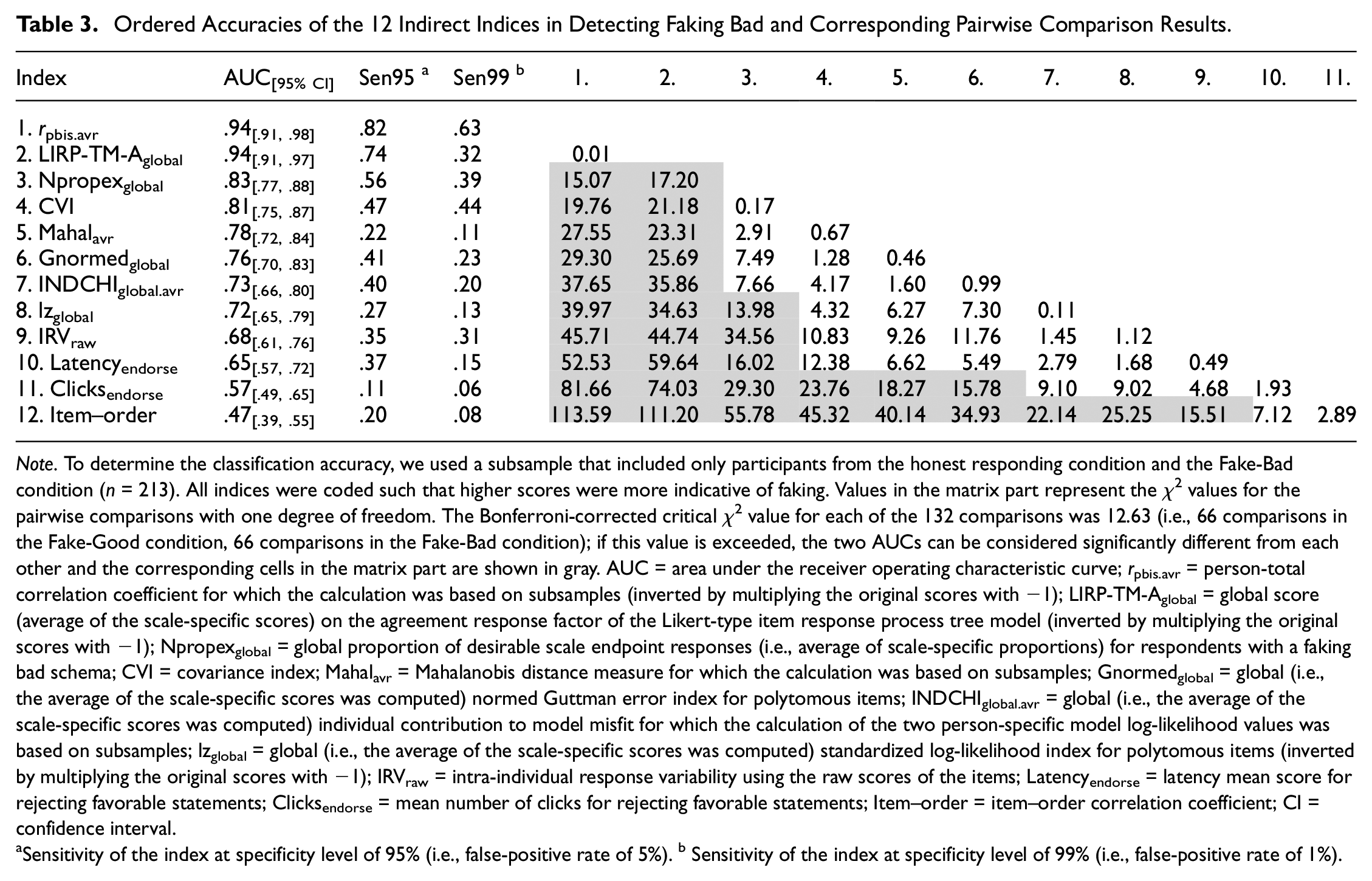
Note. To determine the classification accuracy, we used a subsample that included only participants from the honest responding condition and the Fake-Bad condition (n = 213). All indices were coded such that higher scores were more indicative of faking. Values in the matrix part represent the χ² values for the pairwise comparisons with one degree of freedom. The Bonferroni-corrected critical χ² value for each of the 132 comparisons was 12.63 (i.e., 66 comparisons in the Fake-Good condition, 66 comparisons in the Fake-Bad condition); if this value is exceeded, the two AUCs can be considered significantly different from each other and the corresponding cells in the matrix part are shown in gray. AUC = area under the receiver operating characteristic curve; r_pbis.avr = person-total correlation coefficient for which the calculation was based on subsamples (inverted by multiplying the original scores with −1); LIRP-TM-A_global = global score (average of the scale-specific scores) on the agreement response factor of the Likert-type item response process tree model (inverted by multiplying the original scores with −1); Npropex_global = global proportion of desirable scale endpoint responses (i.e., average of scale-specific proportions) for respondents with a faking bad schema; CVI = covariance index; Mahal_avr = Mahalanobis distance measure for which the calculation was based on subsamples; Gnormed_global = global (i.e., the average of the scale-specific scores was computed) normed Guttman error index for polytomous items; INDCHI_global.avr = global (i.e., the average of the scale-specific scores was computed) individual contribution to model misfit for which the calculation of the two person-specific model log-likelihood values was based on subsamples; lz_global = global (i.e., the average of the scale-specific scores was computed) standardized log-likelihood index for polytomous items (inverted by multiplying the original scores with −1); IRV_raw = intra-individual response variability using the raw scores of the items; Latency_endorse = latency mean score for rejecting favorable statements; Clicks_endorse = mean number of clicks for rejecting favorable statements; Item–order = item–order correlation coefficient; CI = confidence interval.

Sensitivity of the index at specificity level of 95% (i.e., false-positive rate of 5%). ^b Sensitivity of the index at specificity level of 99% (i.e., false-positive rate of 1%).

Pairwise Comparisons Between Impression Management and Indirect Indices

We then addressed the third research question and compared the faking detection performance of each effective indirect index with that of the IM. For detecting respondents that were faking good, LIRP-TM-A_global, Ppropex_global, IRV_raw, and CVI were as accurate as IM (see Table 4). In contrast, Gnormed_global, lz_global, r_pbis.avr, Latency_reject, Mahal_avr, Clicks_reject were not as accurate as IM in detecting faking good among respondents. For detecting respondents that were faking bad, r_pbis.avr, LIRP-TM-A_global, Npropex_global, and CVI were accurate as IM. In contrast, Mahal_avr, Gnormed_global, INDCHI_global.avr, lz_global, IRV_raw, Latency_endorse were not as accurate as IM in detecting faking bad among respondents. In addition, we also examined the indices’ incremental validity beyond IM. These estimates are reported in the Supplemental Material (see Table S5).

Table 4

Pairwise Comparisons Between Impression Management and Indirect Indices Regarding the Detection of Faking Good and Faking Bad

Index	Fake-Good ^a		Fake-Bad ^b
Index	AUC_{[95% CI]}	χ²(1)	AUC_{[95% CI]}	χ²(1)
IM (reference)	.86_{[.81, .91]}		.88_{[.84, .93]}
LIRP-TM-A_global	.86_{[.81, .92]}	0.00	.94_{[.91, .97]}	8.09
Ppropex_global	.85_{[.80, .90]}	0.14	—	—
Npropex_global	—	—	.83_{[.77, .88]}	3.48
IRV_raw	.84_{[.78, .89]}	0.76	.68_{[.61, .76]}	29.71
CVI	.83_{[.77, .89]}	1.26	.81_{[.75, .87]}	5.60
Gnormed_global	.73_{[.66, .80]}	10.09	.76_{[.70, .83]}	11.33
lz_global	.66_{[.59, .74]}	18.91	.72_{[.65, .79]}	17.93
r_pbis.avr	.64_{[.56, .71]}	20.45	.94_{[.91, .98]}	7.02
Latency_reject	.62_{[.55, .70]}	35.05	—	—
Latency_endorse	—	—	.65_{[.57, .72]}	30.52
Mahal_avr	.61_{[.53, .68]}	26.89	.78_{[.72, .84]}	10.13
Clicks_reject	.58_{[.50, .66]}	37.13	—	—
INDCHI_global.avr	—	—	.73_{[.66, .80]}	17.20

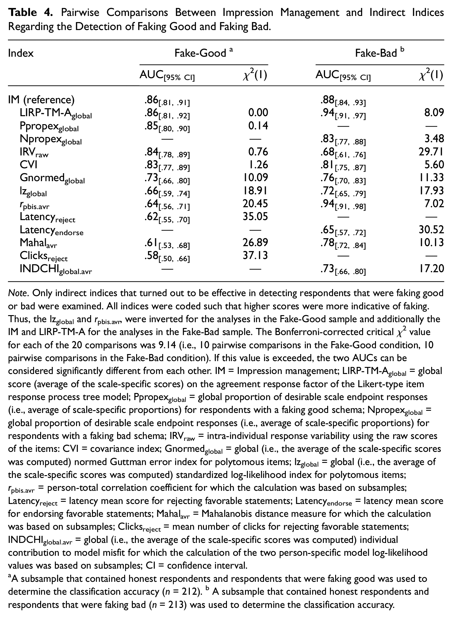
Note. Only indirect indices that turned out to be effective in detecting respondents that were faking good or bad were examined. All indices were coded such that higher scores were more indicative of faking. Thus, the lz_global and r_pbis.avr, were inverted for the analyses in the Fake-Good sample and additionally the IM and LIRP-TM-A for the analyses in the Fake-Bad sample. The Bonferroni-corrected critical χ² value for each of the 20 comparisons was 9.14 (i.e., 10 pairwise comparisons in the Fake-Good condition, 10 pairwise comparisons in the Fake-Bad condition). If this value is exceeded, the two AUCs can be considered significantly different from each other. IM = Impression management; LIRP-TM-A_global = global score (average of the scale-specific scores) on the agreement response factor of the Likert-type item response process tree model; Ppropex_global = global proportion of desirable scale endpoint responses (i.e., average of scale-specific proportions) for respondents with a faking good schema; Npropex_global = global proportion of desirable scale endpoint responses (i.e., average of scale-specific proportions) for respondents with a faking bad schema; IRV_raw = intra-individual response variability using the raw scores of the items: CVI = covariance index; Gnormed_global = global (i.e., the average of the scale-specific scores was computed) normed Guttman error index for polytomous items; lz_global = global (i.e., the average of the scale-specific scores was computed) standardized log-likelihood index for polytomous items; r_pbis.avr = person-total correlation coefficient for which the calculation was based on subsamples; Latency_reject = latency mean score for rejecting favorable statements; Latency_endorse = latency mean score for endorsing favorable statements; Mahal_avr = Mahalanobis distance measure for which the calculation was based on subsamples; Clicks_reject = mean number of clicks for rejecting favorable statements; INDCHI_global.avr = global (i.e., the average of the scale-specific scores was computed) individual contribution to model misfit for which the calculation of the two person-specific model log-likelihood values was based on subsamples; CI = confidence interval.

A subsample that contained honest respondents and respondents that were faking good was used to determine the classification accuracy (n = 212). ^b A subsample that contained honest respondents and respondents that were faking bad (n = 213) was used to determine the classification accuracy.

Comparisons Between IM and Sets of Indirect Indices

Finally, we compared the performance of four sets with that of IM. In the first set, all effective indirect indices were used in combination. In the second set, the three most accurate indices were used in combination. In the third set, the three indices that showed the least averaged absolute correlation with the seven substantive measures were used in combination (see Supplemental Material Table S6). In the fourth set, the three indices that needed the fewest code lines until the final index was obtained (see Supplemental Material Table S7) were used in combination.

Whereas the second and fourth had a detection accuracy comparable to that of IM, the first set even outperformed IM in terms AUC and sensitivity at a false-positive rate of 5%, no matter whether for detecting faking good or bad (see Table 5). To us, however, the performance of the third set was most remarkable. Despite its significantly smaller AUC, this set turned out to have a sensitivity at low false-positive rates comparable to that of IM (see Table 5) and therefore illustrated that indirect indices can be combined such that they are effective in faking detection but only weakly correlated with the substantive measures (i.e., ranging from .11 to .23).

Table 5

Pairwise Comparisons Between Impression Management and Sets of Indirect Indices Regarding the Detection of Faking Good and Faking Bad

Index	AUC comparison		Sen95 comparison ^a		Sen99 comparison ^b
Index	AUC_{[95% CI]}	χ²(1)	Sen95	Z	Sen99	Z
Fake-Good ^c
IM (reference)	.86_{[.81, .91]}		.50		.34
Set 1 (all effective indirect indices)	.96_{[.94, .98]}	16.36	.82	−3.80	.68	−2.16
Set 2 (LIRP-TM-A_global, Ppropex_global, IRV_raw)	.91_{[.87, .95]}	3.84	.69	−2.40	.60	−2.20
Set 3 (lz_global, Gnormed_global, Clicks_reject)	.73_{[.66, .80]}	10.43	.42	0.75	.26	0.53
Set 4 (IRV_raw, Mahal_avr, Ppropex_global)	.85_{[.80, .90]}	0.20	.51	−0.21	.48	−1.16
Fake-Bad ^d
IM (reference)	.88_{[.84, .93]}		.50		.33
Set 1 (all effective indirect indices)	.97_{[.95 .99]}	16.81	.93	−4.20	.71	−2.92
Set 2 (r_pbis.avr, LIRP-TM-A_global, Npropex_global)	.96_{[.94, .98]}	13.66	.90	−3.28	.54	−1.31
Set 3 (lz_global, Mahal_avr, INDCHI_global.avr)	.81_{[.75, .87]}	5.72	.39	1.06	.18	1.70
Set 4 (IRV_raw, Mahal_avr, Npropex_global)	.90_{[.86, .94]}	0.38	.54	−0.36	.35	−0.15

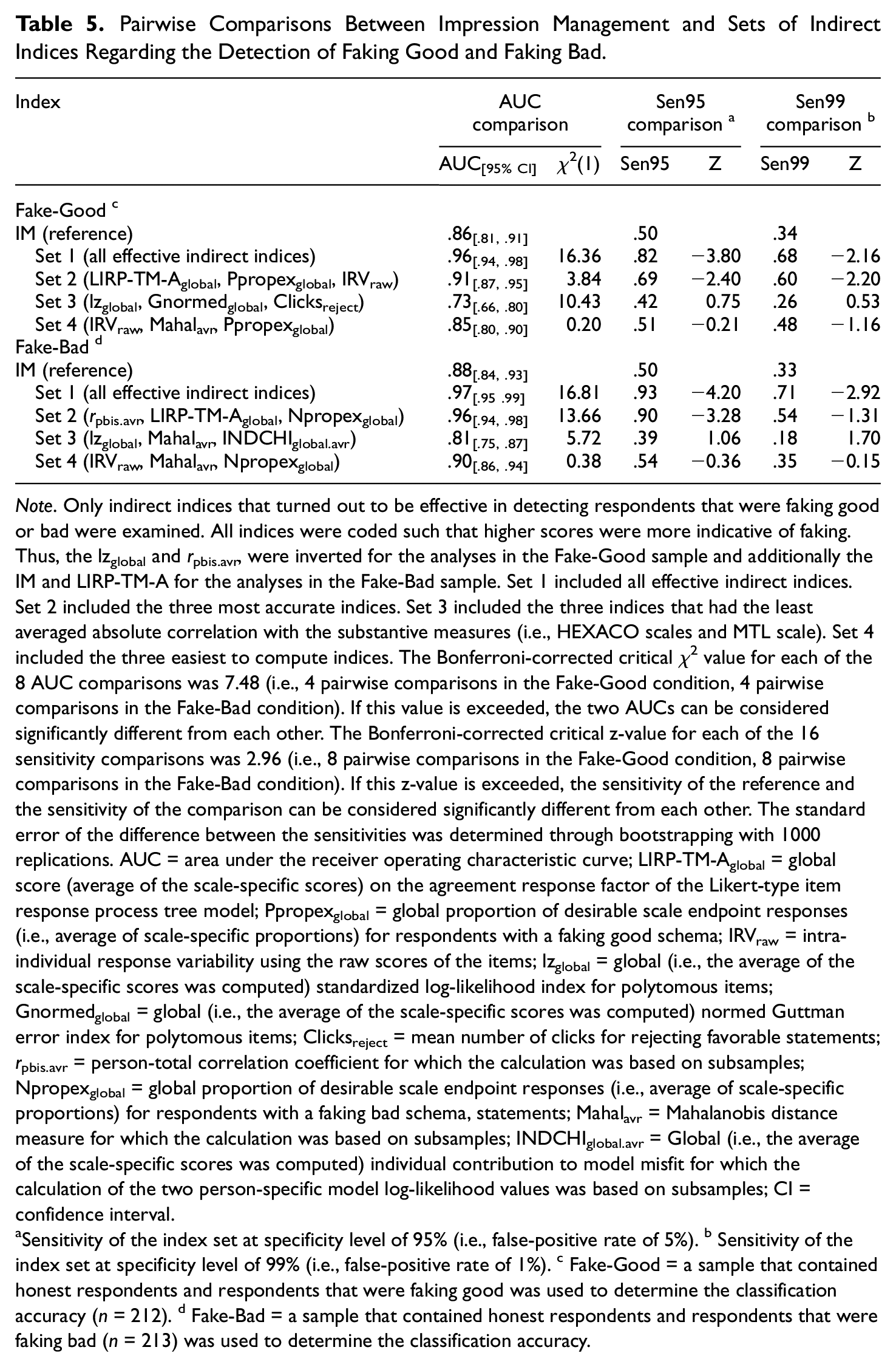
Note. Only indirect indices that turned out to be effective in detecting respondents that were faking good or bad were examined. All indices were coded such that higher scores were more indicative of faking. Thus, the lz_global and r_pbis.avr, were inverted for the analyses in the Fake-Good sample and additionally the IM and LIRP-TM-A for the analyses in the Fake-Bad sample. Set 1 included all effective indirect indices. Set 2 included the three most accurate indices. Set 3 included the three indices that had the least averaged absolute correlation with the substantive measures (i.e., HEXACO scales and MTL scale). Set 4 included the three easiest to compute indices. The Bonferroni-corrected critical χ² value for each of the 8 AUC comparisons was 7.48 (i.e., 4 pairwise comparisons in the Fake-Good condition, 4 pairwise comparisons in the Fake-Bad condition). If this value is exceeded, the two AUCs can be considered significantly different from each other. The Bonferroni-corrected critical z-value for each of the 16 sensitivity comparisons was 2.96 (i.e., 8 pairwise comparisons in the Fake-Good condition, 8 pairwise comparisons in the Fake-Bad condition). If this z-value is exceeded, the sensitivity of the reference and the sensitivity of the comparison can be considered significantly different from each other. The standard error of the difference between the sensitivities was determined through bootstrapping with 1000 replications. AUC = area under the receiver operating characteristic curve; LIRP-TM-A_global = global score (average of the scale-specific scores) on the agreement response factor of the Likert-type item response process tree model; Ppropex_global = global proportion of desirable scale endpoint responses (i.e., average of scale-specific proportions) for respondents with a faking good schema; IRV_raw = intra-individual response variability using the raw scores of the items; lz_global = global (i.e., the average of the scale-specific scores was computed) standardized log-likelihood index for polytomous items; Gnormed_global = global (i.e., the average of the scale-specific scores was computed) normed Guttman error index for polytomous items; Clicks_reject = mean number of clicks for rejecting favorable statements; r_pbis.avr = person-total correlation coefficient for which the calculation was based on subsamples; Npropex_global = global proportion of desirable scale endpoint responses (i.e., average of scale-specific proportions) for respondents with a faking bad schema, statements; Mahal_avr = Mahalanobis distance measure for which the calculation was based on subsamples; INDCHI_global.avr = Global (i.e., the average of the scale-specific scores was computed) individual contribution to model misfit for which the calculation of the two person-specific model log-likelihood values was based on subsamples; CI = confidence interval.

Sensitivity of the index set at specificity level of 95% (i.e., false-positive rate of 5%). ^b Sensitivity of the index set at specificity level of 99% (i.e., false-positive rate of 1%). ^c Fake-Good = a sample that contained honest respondents and respondents that were faking good was used to determine the classification accuracy (n = 212). ^d Fake-Bad = a sample that contained honest respondents and respondents that were faking bad (n = 213) was used to determine the classification accuracy.

Discussion

This article had two major aims, to examine how well indices of a representative selection of 12 conceptionally different indirect faking detection indices perform compared with each other, and to examine how well the selected indirect indices perform (individually and jointly) compared with an established direct faking measure or validity scale. By examining these issues, we wanted to provide researchers with a differentiated basis upon which they can select and combine indirect indices for detecting faking in their data.

Which Subversion of an Indirect Index Should be Calculated?

Certain subversions of indirect indices performed better in faking detection than others. First, global versions of indices performed generally better than their scale-specific counterparts (i.e., LIRP-TM, Ppropex, lz, Gnormed). The only exception was the index INDCHI. In the case of INDCHI, versions that were calculated on the basis of specific scales (e.g., extraversion, agreeableness) tended to be more accurate in faking detection than the global INDCHI version. For most of the indices that allow the calculation of global and scale-specific versions, it, therefore, seems to be a safe choice to base the index calculation on more and different facets, especially because it may not always be clear which of the study scales will be saturated most with “desirable variance.”

Second, IRV_raw performed better than IRV_scored. This result was unexpected for us in two ways. For one, because the IRV that was based on scored items (i.e., all into positivity; Holden & Marjanovic, 2021, p. 3) turned out to be completely ineffective. For another, because the alternative IRV measure that was based on raw item scores (see Goldammer et al., 2020) turned out to screen in the “wrong” direction. Contrary to what we thought and in line with Holden and Marjanovic’s (2021) expectation, larger IRV values were more indicative of both forms of faking; however, larger IRV values tended to be more indicative of faking good than faking bad (see Tables 2 and 3). Thus, instead of hyper-consistent responding, extreme responding was the response pattern that was indicative of faking, and IRV_raw was the version that captured this extremity best. In contrast to our categorization, therefore, IRV_raw may be better regarded as another measure for extreme responding, which seems to be supported by the strong correlation between IRV_raw and other measures of extreme responding (e.g., LIRP-TM, Ppropex, see Supplemental Material Tables S2, S3, S12, S22).

Third, index calculations based on subsamples tended to be more accurate than calculations in which the indices were obtained at once in the total sample. This primarily concerned indices that involved an explicit comparison of each respondent’s response vector with that of the sample norm (i.e., Mahal, r_pbis, INDCHI). Thus, if the norm is not set in maximal favor for honest or non-faking respondents, these indices might be less effective or even detect the wrong targets (i.e., honest or non-faking participants). Indices like Mahal, r_pbis, and INDCHI should therefore only be used if it can be assumed that the majority of the sample responded honestly, or if a norm sample is at hand that can be used for the subsample-based calculations of the indices.

Fourth, measures of scale endpoint responses in which the respondent’s faking schema was taken into account (i.e., Ppropex, Npropex) generally performed better than the measure in which all endpoint responses were counted irrespective of the respondent’s faking schema (i.e., IDpropex). The somewhat greater coding effort that has to be undertaken when calculating the tailored endpoint response measures (i.e., Ppropex, Npropex) tends to pay off in terms of a higher detection rate.

Finally, scores on the agreement and midpoint LIRP-TM response factors tended to be a bit more accurate than scores on the extremity LIRP-TM response factor. The poorer performance of the extremity factor is not surprising, insofar as this score is based on a pseudo-item coding schema that is almost identical to the one that is used for the calculation of the IDpropex. As in the case of the measures of scale endpoint responses, using tailored measures also tends to pay off in the case of the LIRP-TM factors (e.g., LIRP-TM-A).

Which Indirect Index Performs Best?

The Top Three Indices

Certain indirect indices performed better in faking detection than others. Of the 12 indices examined, LIRP-TM-A_global, Ppropex_global, and CVI were the only indirect indices that performed better than chance and that reached a comparable detection accuracy for detecting faking good and bad as the direct faking measure (see Table 6). We therefore recommend without any reservation using LIRP-TM-A_global, Ppropex_global, and CVI for faking detection.

Table 6

Summary of Findings on the Effectiveness of the Indices and Recommendations for Further Use of the Indices

Index	Does the index perform better than chance?		Performance compared with direct faking measure		Averaged absolute correlation with substantive scales
Index	Fake-Good	Fake-Bad	Fake-Good	Fake-Bad	Fake-Good	Fake-Bad	Code lines	Norm required	Recommendation
LIRP-TM-A_global	Yes	Yes	Equal	Equal	0.58	0.59	1,186	No	Use
Ppropex_global	Yes	Yes	Equal	Equal	0.49	0.55	62	No	Use
CVI	Yes	Yes	Equal	Equal	0.56	0.63	230	Yes	Use
IRV_raw	Yes	Yes	Equal	Worse	0.43	0.47	6	No	Use
Latency	Yes	Yes	Worse	Worse	0.23	0.27	355	Yes	Use
Gnormed_global	Yes	Yes	Worse	Worse	0.09	0.24	224	No	Use
lz_global	Yes	Yes	Worse	Worse	0.20	0.11	224	No	Use
r _{pbis avr}	Yes	Yes	Worse	Equal	0.35	0.49	73	Recommended	Use
Mahal_avr	Yes	Yes	Worse	Worse	0.14	0.19	43	Recommended	Use
INDCHI	No	Yes	Worse	Worse	0.14	0.22	755	Recommended	Use with caution
Clicks	Yes	No	Worse	Worse	0.11	0.09	109	Yes	Use with caution
Item–order	No	No	Worse	Worse	0.11	0.17	125	No	Do not use

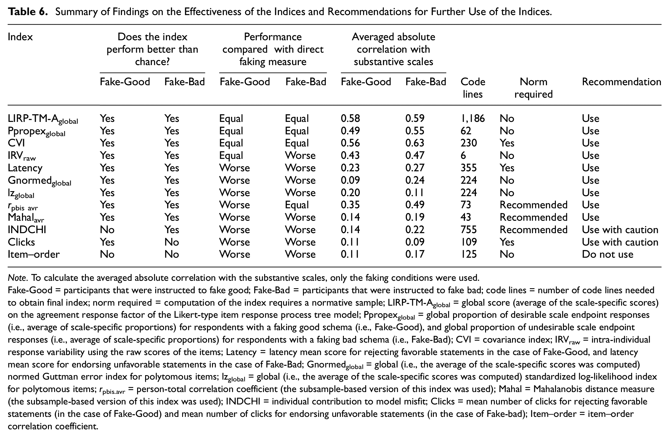
Note. To calculate the averaged absolute correlation with the substantive scales, only the faking conditions were used.

Fake-Good = participants that were instructed to fake good; Fake-Bad = participants that were instructed to fake bad; code lines = number of code lines needed to obtain final index; norm required = computation of the index requires a normative sample; LIRP-TM-A_global = global score (average of the scale-specific scores) on the agreement response factor of the Likert-type item response process tree model; Ppropex_global = global proportion of desirable scale endpoint responses (i.e., average of scale-specific proportions) for respondents with a faking good schema (i.e., Fake-Good), and global proportion of undesirable scale endpoint responses (i.e., average of scale-specific proportions) for respondents with a faking bad schema (i.e., Fake-Bad); CVI = covariance index; IRV_raw = intra-individual response variability using the raw scores of the items; Latency = latency mean score for rejecting favorable statements in the case of Fake-Good, and latency mean score for endorsing unfavorable statements in the case of Fake-Bad; Gnormed_global = global (i.e., the average of the scale-specific scores was computed) normed Guttman error index for polytomous items; lz_global = global (i.e., the average of the scale-specific scores was computed) standardized log-likelihood index for polytomous items; r_pbis.avr = person-total correlation coefficient (the subsample-based version of this index was used); Mahal = Mahalanobis distance measure (the subsample-based version of this index was used); INDCHI = individual contribution to model misfit; Clicks = mean number of clicks for rejecting favorable statements (in the case of Fake-Good) and mean number of clicks for endorsing unfavorable statements (in the case of Fake-bad); Item–order = item–order correlation coefficient.

Second-Place Indices

In the ranking, following the top-performing indices, there is a group of indices (i.e., IRV_raw, Latency, Gnormed_global, lz_global, r_pbis.avr, Mahal_avr) that performed better than chance but did not reach the accuracy of the direct measure when the aim is to detect faking good and/or faking bad (see Table 6). When using these second-place indices for faking detection, we therefore recommend combining them with other effective indirect indices. This should help to obtain a comparable level of accuracy as the direct faking measure. Moreover, the detection accuracy of some indices of this group may even improve further if certain contextual factors are designed in their favor.

For instance, it has been shown that person-fit statistics like lz and Gnormed have a higher detection rate of aberrant responding if more items per unidimensional construct are used (Karabatsos, 2003). In contrast to Karabatsos (2003), who considered 17 items per construct as short and a test with 65 items as long, we only used 10 items on average per dimension across the studies, which may partially explain why lz and Gnormed showed only mediocre performance in our study. Similarly, it has been suggested that latency measures will be more accurate if more test items are used, because longer tests would give the test-taker more chances to provide schema-inconsistent responses, which in turn would result in a more reliable latency index (Röhner & Holden, 2022).

Third-Place Indices

The performance of the INDCHI and the clicks per item index was only partially convincing. Whereas the INDCHI was only effective in detecting faking bad, the click index was only marginally effective in detecting faking good. We, therefore, recommend using these indices only for detecting the faking form, for which they have shown to be effective in our study. In addition, we strongly recommend using the INDCHI and the click index in combination with other effective indirect indices, such that the accuracy level of the direct faking measure can at least be approached.

Last-Place Index

The last-place index is item–order correlation. This index turned out to be ineffective in detecting both faking good and faking bad (see Table 6). The poor performance of this index was unexpected and stands in contrast to Holden et al.’s (2017) results showing that the index effectively discriminated between faking and non-faking respondents in five samples of university students. Considering these findings, we, therefore, recommend not using the Item–order index for faking detection until future experimental studies provide evidence for its utility and clarify under what conditions the index performs best.

What is the Benefit of Using Indirect Indices in Combination?

We would like to highlight two observations that we made when we examined how sets of indirect indices performed in faking detection. First, using indirect indices in combination, especially those from different categories (e.g., measures of deviating response processes, measures of response extremity, consistency-based measures), tended to go along with better detection rates than when using these indices individually. Second, using indirect indices in combination resulted in comparable and, in some cases, even better detection rates than when using direct faking measures. Therefore, using indirect indices in combination generally seems to be beneficial for faking detection.

Besides these general positive features, each of the four sets that we examined had its unique quality. For instance, whereas the set in which all effective (or the best-performing) indices were used in combination had the advantage of being most accurate and sensitive at low false-positive rates, the set in which indices like IRV and Ppropex were used in combination had the advantage that only little coding effort was needed until the screening could start (see Table 6). To us, however, the most interesting advantage came with the set in which indices were used in combination that were the least correlated with the substantive measures (see Table 6). Because such a set is unconfounded with substance, it could have also been used to partial faking variance without losing substance. This, in turn, may offer new possibilities for researchers who want to take into account the impact of faking when estimating the predictive validity of personality tests used in personal selection procedures.

Limitations and Future Research Directions

There are several limitations of this research that need to be mentioned. First, the items were presented as single statements to which the respondents had to indicate their agreement, which is commonly known as a Likert-type scale response format. Our findings regarding the indirect indices’ utility for faking detection are therefore only valid for this type of response format. Although the Likert-type scale may be a popular and convenient response format, when it comes to personality assessment in high-stakes situations, questionnaires with a forced-choice response format tend to be the more faking-resistant (Cao & Drasgow, 2019). Nevertheless, the forced-choice format does not prevent faking completely (Cao & Drasgow, 2019, p. 1359). It would therefore be interesting to see whether the indirect indices presented here can be adapted to forced-choice response formats, and whether the adapted indices have the same accuracy in faking detection as their counterparts in Likert-type scale format.

Second, we used IM as a direct faking measure against which we compared the indirect indices. Hence, the relative performance of the indirect indices may depend on our selection. For instance, it may be argued that certain indirect indices only performed that well or badly because they were compared with this specific direct measure (i.e., IM). Thus, the generalizability of our findings may be limited because of the specific direct faking measure that we used. Therefore, future studies should extend our work and examine the faking detection performance of indirect indices in comparison to other direct faking measures.

Third, some indirect indices may have just performed that well (or poorly) because we examined them under conditions that were favorable (or unfavorable) for them. For example, indices that we labeled as second-place indices might have performed better if the test and faking conditions had been different. In this regard, a reviewer rightfully argued that the faking instruction may have altered the faking process itself. Thus, the generalizability of our findings may be limited because of the specific test and faking conditions that we examined. Future studies should therefore systematically manipulate the test and faking conditions and examine under what conditions the different indirect indices perform best.

Fourth, our results suggest that using indirect indices in combination goes along with increased faking detection rates. To estimate and test the joint effect of sets of indirect indices, we used the predicted values of logit regression models. However, there are other approaches using indirect indices jointly that may even be associated with higher detection rates. For instance, Goldammer et al. (2020) examined the multiple hurdle (i.e., using indices sequentially at predefined cut-scores) and the latent-class analysis approach (i.e., inferring the latent group membership of fakers and non-fakers by using indirect indices as latent class indicators) for the overall classification of careful and careless responders. Future studies could therefore examine which of these approaches using indirect indices in combination is best for faking detection.

Finally, we examined the utility of indirect indices only in the context of self-reported personality measures. This, of course, raises the question as to whether these indirect indices can be used to detect faking in different rating contexts. For instance, it would be interesting to examine whether these indirect indices detect faking when subordinates rate their supervisor in a positively biased way, or whether they even allow faking detection when pre-election polls are purposefully misreported.

Conclusion

To detect faking in questionnaires, a common strategy has been to add what are called direct faking measures or validity scales to the regular questionnaire. However, these direct measures can be faked as well, lengthen the questionnaire, and usually correlate strongly with substantive scales. As our results suggest, a better approach to assess respondents’ faking can therefore be the use of indirect indices. This is because, first, they cannot be detected by the test-taker. Second, their usage does not require changes to the regular questionnaire. Third, their usage resulted in comparable and, in some cases, even better detection rates than the usage of direct faking measures. Finally, some of these indirect indices might even be used as control variables to partial faking variance from response sets without losing substance, as they are only minimally correlated with the substantive scales. We, therefore, encourage researchers to use indirect indices instead of direct measures when they aim to detect faking in their data.

Supplemental Material

sj-docx-1-epm-10.1177_00131644231209520 – Supplemental material for On the Utility of Indirect Methods for Detecting Faking

Supplemental material, sj-docx-1-epm-10.1177_00131644231209520 for On the Utility of Indirect Methods for Detecting Faking by Philippe Goldammer, Peter Lucas Stöckli, Yannik Andrea Escher, Hubert Annen and Klaus Jonas in Educational and Psychological Measurement

Footnotes

Declaration of Conflicting Interests

The authors declared no potential conflicts of interest with respect to the research, authorship, and/or publication of this article.

Funding

The authors received no financial support for the research, authorship, and/or publication of this article.

ORCID iDs

Philippe Goldammer

Yannik Andrea Escher

Hubert Annen

Klaus Jonas

Supplemental Material

Supplemental material for this article is available online.

Notes

References

Alliger

G. M.

Lilienfeld

S. O.

Mitchell

K. E.

(1996). The susceptibility of overt and covert integrity tests to coaching and faking. Psychological Science, 7(1), 32–39. https://doi.org/10.1111/j.1467-9280.1996.tb00663.x

Arthur

Hagen

George

Jr. (2021). The lazy or dishonest respondent: Detection and prevention. Annual Review of Organizational Psychology and Organizational Behavior, 8, 105–137. https://doi.org/10.1146/annurev-orgpsych-012420-055324

Ashton

M. C.

Lee

(2009). The HEXACO-60: A short measure of the major dimensions of personality. Journal of Personality Assessment, 91(4), 340–345. https://doi.org/10.1080/00223890902935878

Böckenholt

(2012). Modeling multiple response processes in judgment and choice. Psychological Methods, 17(4), 665–678. https://doi.org/10.1037/a0028111

Böckenholt

(2017). Measuring response styles in Likert items. Psychological Methods, 22(1), 69–83. https://doi.org/10.1037/met0000106

Borgatta

E. F.

Glass

D. C.

(1961). Personality concomitants of extreme response set (ERS). Journal of Social Psychology, 55, 213–221. https://doi.org/10.1080/00224545.1961.9922176

Bowling

N. A.

Gibson

A. M.

Houpt

J. W.

Brower

C. K.

(2021). Will the questions ever end? Person-level increases in careless responding during questionnaire completion. Organizational Research Methods, 24(4), 718–738. https://doi.org/10.1177/1094428120947794

Burns

G. N.

Christiansen

N. D.

(2011). Methods of measuring faking behavior. Human Performance, 24(4), 358–372. https://doi.org/10.1080/08959285.2011.597473

Cao

Drasgow

(2019). Does forcing reduce faking? A meta-analytic review of forced-choice personality measures in high-stakes situations. Journal of Applied Psychology, 104(11), 1347–1368. https://doi.org/10.1037/apl0000414

10.

Chan

K. Y.

Drasgow

(2001). Toward a theory of individual differences and leadership: Understanding the motivation to lead. Journal of Applied Psychology, 86(3), 481–498. https://doi.org/10.1037/0021-9010.86.3.481

11.

Christiansen

N. D.

Robie

Burns

G. N.

Speer

A. B.

(2017). Using item-level covariance to detect response distortion on personality measures. Human Performance, 30(2-3), 116–134. https://doi.org/10.1080/08959285.2017.1319366

12.

Connelly

B. S.

Chang

(2016). A meta-analytic multitrait multirater separation of substance and style in social desirability scales. Journal of Personality, 84(3), 319–334. https://doi.org/10.1111/jopy.12161

13.

Curran

P. G.

(2016). Methods for the detection of carelessly invalid responses in survey data. Journal of Experimental Social Psychology, 66, 4–19. https://doi.org/10.1016/j.jesp.2015.07.006

14.

DeLong

E. R.

DeLong

D. M.

Clarke-Pearson

D. L.

(1988). Comparing the areas under two or more correlated receiver operating characteristic curves: A nonparametric approach. Biometrics, 44(3), 837–845. https://doi.org/10.2307/2531595

15.

Donlon

T. F.

Fischer

F. E.

(1968). An index of an individual’s agreement with group-determined item difficulties. Educational and Psychological Measurement, 28(1), 105–113. https://doi.org/10.1177/001316446802800110

16.

Drasgow

Levine

M. V.

Williams

E. A.

(1985). Appropriateness measurement with polychotomous item response models and standardized indices. British Journal of Mathematical and Statistical Psychology, 38(1), 67–86. https://doi.org/10.1111/j.2044-8317.1985.tb00817.x

17.

Emons

W. H.

(2008). Nonparametric person-fit analysis of polytomous item scores. Applied Psychological Measurement, 32(3), 224–247. https://doi.org/10.1177/0146621607302479

18.

Felfe

Elprana

Gatzka

Stiehl

(2012). FÜMO. Hamburger Führungsmotivationsinventar [FÜMO. Hamburg inventory of leadership motivation]. Hogrefe.

19.

Goffin

R. D.

Boyd

A. C.

(2009). Faking and personality assessment in personnel selection: Advancing models of faking. Canadian Psychology, 50(3), 151–160. https://doi.org/10.1037/a0015946

20.

Goffin

R. D.

Christiansen

N. D.

(2003). Correcting personality tests for faking: A review of popular personality tests and an initial survey of researchers. International Journal of Selection and Assessment, 11(4), 340–344. https://doi.org/10.1111/j.0965-075X.2003.00256.x

21.

Goldammer

Annen

Stöckli

P. L.

Jonas

(2020). Careless responding in questionnaire measures: Detection, impact, and remedies. The Leadership Quarterly, 31(4), Article 101384. https://doi.org/10.1016/j.leaqua.2020.101384

22.

Holden

R. R.

Book

A. S.

(2012). Faking does distort self-report personality assessment. In Ziegler

MacCann

Roberts

R. D.

(Eds.), New perspectives on faking in personality assessment (pp. 71–84). Oxford University Press.

23.

Holden

R. R.

Kroner

D. G.

Fekken

G. C.

Popham

S. M.

(1992). A model of personality test item response dissimulation. Journal of Personality and Social Psychology, 63(2), 272–279.

24.

Holden

R. R.

Lambert

C. E.

D’Agata

M. T.

Book

A. S.

(2017). Response patterns for the identification of fakers: Detecting drifting dissimulators. Personality and Individual Differences, 108, 195–199. https://doi.org/10.1016/j.paid.2016.12.029

25.

Holden

R. R.

Marjanovic

(2021). Faking on a self-report personality inventory: Indiscriminate, discriminate, or hyper-discriminate responding? Personality and Individual Differences, 169, Article 109768. https://doi.org/10.1016/j.paid.2019.109768

26.

Huang

J. L.

Curran

P. G.

Keeney

Poposki

E. M.

DeShon

R. P.

(2012). Detecting and deterring insufficient effort responding to surveys. Journal of Business and Psychology, 27(1), 99–114. https://doi.org/10.1007/s10869-011-9231-8

27.

Karabatsos

(2003). Comparing the aberrant response detection performance of thirty-six person-fit statistics. Applied Measurement in Education, 16(4), 277–298. https://doi.org/10.1207/S15324818AME1604_2

28.

Kiefer

Benit

(2016). What is applicant faking behavior? A review on the current state of theory and modeling techniques. Journal of European Psychology Students, 7(1), 9–19. https://doi.org/10.5334/jeps.345

29.

König

C. J.

Mura

Schmidt

(2015). Applicants’ strategic use of extreme or midpoint responses when faking personality tests. Psychological Reports, 117(2), 429–436. https://doi.org/10.2466/03.02.PR0.117c21z2

30.

Kroger

R. O.

Turnbull

(1975). Invalidity of validity scales: The case of the MMPI. Journal of Consulting and Clinical Psychology, 43(1), 48–55. https://doi.org/10.1037/h0076266

31.

Lambert

C. E.

Arbuckle

S. A.

Holden

R. R.

(2016). The Marlowe–Crowne Social Desirability Scale outperforms the BIDR Impression Management Scale for identifying fakers. Journal of Research in Personality, 61, 80–86. https://doi.org/10.1016/j.jrp.2016.02.004

32.

Landers

R. N.

Sackett

P. R.

Tuzinski

K. A.

(2011). Retesting after initial failure, coaching rumors, and warnings against faking in online personality measures for selection. Journal of Applied Psychology, 96(1), 202–210. https://doi.org/10.1037/a0020375

33.

Lanz

Thielmann

Gerpott

F. H.

(2022). Are social desirability scales desirable? A meta-analytic test of the validity of social desirability scales in the context of prosocial behavior. Journal of Personality, 90(2), 203–221. https://doi.org/10.1111/jopy.12662

34.

Levashina

Weekley

J. A.

Roulin

Hauck

(2014). Using blatant extreme responding for detecting faking in high-stakes selection: Construct validity, relationship with general mental ability, and subgroup differences. International Journal of Selection and Assessment, 22(4), 371–383. https://doi.org/10.1111/ijsa.12084

35.

Mahalanobis

P. C.

(1936). On the generalized distance in statistics. Proceedings of the National Institute of Sciences of India, 2(1), 49–55.

36.

Meijer

R. R.

Niessen

A. S. M.

Tendeiro

J. N.

(2016). A practical guide to check the consistency of item response patterns in clinical research through person-fit statistics: Examples and a computer program. Assessment, 23(1), 52–62. https://doi.org/10.1177/1073191115577800

37.

Musch

Brockhaus

Bröder

(2002). Ein Inventar zur Erfassung von zwei Faktoren sozialer Erwünschtheit [An inventory for the assessment of two factors of social desirability]. Diagnostica, 48(3), 121–129. https://doi.org/10.1026/0012-1924.48.3.121

38.

Niessen

A. S. M.

Meijer

R. R.

Tendeiro

J. N.

(2016). Detecting careless respondents in web-based questionnaires: Which method to use? Journal of Research in Personality, 63, 1–11. https://doi.org/10.1016/j.jrp.2016.04.010

39.

Paulhus

D. L.

(1994). Balanced Inventory of Desirable Responding: Reference manual for BIDR version 6 [Unpublished manuscript]. University of British Columbia, Vancouver, BC, Canada.

40.

Paulhus

D. L.

(2002). Socially desirable responding: The evolution of a construct. In Braun

H. I.

Jackson

D. N.

Wiley

D. E.

(Eds.), The role of constructs in psychological and educational measurement (pp. 49–69). Lawrence Erlbaum.

41.

Reise

S. P.

Widaman

K. F.

(1999). Assessing the fit of measurement models at the individual level: A comparison of item response theory and covariance structure approaches. Psychological Methods, 4(1), 3–21. https://doi.org/10.1037/1082-989X.4.1.3

42.

Röhner

Holden

R. R.

(2022). Challenging response latencies in faking detection: The case of few items and no warnings. Behavior Research Methods, 54(1), 324–333. https://doi.org/10.3758/s13428-021-01636-z

43.

Röhner

Schröder-Abé

Schütz

(2011). Exaggeration is harder than understatement, but practice makes perfect! Faking success in the IAT. Experimental Psychology, 58(6), 464–472. https://doi.org/10.1027/1618-3169/a000114

44.

Röhner

Thoss

Schütz

(2022). Lying on the dissection table: Anatomizing faked responses. Behavior Research Methods, 54(6), 2878–2904. https://doi.org/10.3758/s13428-021-01770-8

45.

StataCorp. (2021). Stata statistical software: Release 17. StataCorp LLC.

46.

Sun

Zhang

Cao

Drasgow

(2021). Faking detection improved: Adopting a Likert item response process tree model. Organizational Research Methods, 25(3), 490–512. https://doi.org/10.1177/10944281211002904

47.

Swets

J. A.

(1986). Indices of discrimination or diagnostic accuracy: Their ROCs and implied models. Psychological Bulletin, 99(1), 100–117. https://doi.org/10.1037/0033-2909.99.1.100

48.

Tabachnick

B. G.

Fidell

L. S.

(2007). Using multivariate statistics (5th ed.). Pearson.

49.

Tracey

T. J. G.

(2016). A note on socially desirable responding. Journal of Counseling Psychology, 63(2), 224–232. https://doi.org/10.1037/cou0000135

Supplementary Material

Please find the following supplemental material available below.

For Open Access articles published under a Creative Commons License, all supplemental material carries the same license as the article it is associated with.

For non-Open Access articles published, all supplemental material carries a non-exclusive license, and permission requests for re-use of supplemental material or any part of supplemental material shall be sent directly to the copyright owner as specified in the copyright notice associated with the article.

0.00 MB

0.42 MB