Sage Journals: Discover world-class research

Abstract

Multiple imputation (MI) is one of the recommended techniques for handling missing data in ordinal factor analysis models. However, methods for computing MI-based fit indices under ordinal factor analysis models have yet to be developed. In this short note, we introduced the methods of using the standardized root mean squared residual (SRMR) and the root mean square error of approximation (RMSEA) to assess the fit of ordinal factor analysis models with multiply imputed data. Specifically, we described the procedure for computing the MI-based sample estimates and constructing the confidence intervals. Simulation results showed that the proposed methods could yield sufficiently accurate point and interval estimates for both SRMR and RMSEA, especially in conditions with larger sample sizes, less missing data, more response categories, and higher degrees of misfit. Based on the findings, implications and recommendations were discussed.

Keywords

missing data multiple imputation ordinal factor analysis model model fit SRMR RMSEA

Ordinal factor analysis models (Muthén, 1993; Muthén et al., 1997) are widely used in social and behavioral sciences when latent constructs are measured by instruments with ordinal response scales (e.g., Likert-type rating scales; Likert, 1932). For any statistical model, assessment of model-data fit is a crucial issue because statistical inferences and substantive conclusions based on poorly fitting models are very likely to be misleading (Saris et al., 2009). When fitting ordinal factor analysis models, the model fit is typically assessed using the goodness of fit indices under the structural equation modeling (SEM) framework. A host of SEM fit indices, such as the root mean squared error of approximation (RMSEA; Steiger & Lind, 1980), the comparative fit index (CFI; Bentler, 1990), the Tucker–Lewis index (TLI; Bentler & Bonett, 1980; Tucker & Lewis, 1973), and the standardized root mean squared residual (SRMR; Jöreskog & Sörbom, 1988) have been widely used and routinely reported when fitting ordinal factor analysis models using popular SEM software (e.g., Mplus).

It is noted that most fit indices were first introduced under the SEM models with continuous indicators, where maximum likelihood (ML) is the most commonly used estimation method (Jöreskog, 1969; Maydeu-Olivares, 2017b). However, estimation methods based on least squares, such as the unweighted least squares (ULS; estimator = ULSMV in Mplus) or the diagonally weighted least squares (DWLS; estimator = WLSMV in Mplus) are traditionally used under ordinal factor analysis models (Jöreskog & Sörbom, 1988; Muthén, 1993; Muthén et al., 1997). Researchers have indicated that the SEM fit indices can be substantially influenced by the choice of estimation methods (Shi & Maydeu-Olivares, 2020; Xia & Yang, 2019). Existing knowledge on fit indices, such as their computational formulas and conventional cutoffs, obtained using ML with continuous data may not generalize to scenarios where ordinal factor analysis models are used (Savalei, 2017, 2021).

Methodological research has shed light on providing guidelines for better estimating and interpreting fit indices under ordinal factor analysis. For example, statistical theories for computing point estimates and confidence intervals (CIs) for SRMR and RMSEA under ordinal data have been introduced by Shi, Maydeu-Olivares and Rosseel (2020) and Lai (2020). Moreover, given that the conventional cutoffs for indices were derived under the ML estimation method, alternative procedures have been proposed to align fit indices (e.g., RMSEA, CFI) for ordinal factor analysis with values that would have been obtained if the data were not discretized and analyzed using ML (Savalei, 2021).

Despite the above advances, there are still unaddressed issues in assessing the goodness of fit of ordinal factor analysis models. One of the major challenges is how to estimate the fit indices in the presence of missing data. Missing data are very likely to occur in psychological and educational studies. For example, Peng et al. (2006) conducted a review of 1,666 studies from 11 major education and psychology journals. Among the articles they reviewed, 48% exhibited clear evidence of missing data, and approximately 16% did not provide missing data information.

It has been widely known among researchers that modern techniques for handling missing data, such as the full information maximum likelihood (FIML; Allison, 1987; Arbuckle, 1996; Finkbeiner, 1979) and multiple imputation (MI; Rubin, 1976, 1987), are recommended. Specifically, using the typology developed by Rubin (1976), when the missing data mechanism is either missing at random (MAR) or missing completely at random (MCAR), FIML and MI could outperform the traditional missing data methods (e.g., listwise deletion or pairwise deletion) by yielding less biased and/or more efficient parameter estimates (Enders, 2010).

Ordinal factor analysis models can be estimated using FIML under the framework of item response theory (IRT). However, although the fit indices for ordinal factor analysis models using FIML have been developed under the IRT framework (e.g., Maydeu-Olivares & Joe, 2005), they are computationally burdensome and have not been implemented in SEM software. Moreover, as integration over latent factors is required (Baker & Kim, 2004; Kamata & Bauer, 2008), using FIML to estimate the ordinal factor analysis model itself could be computationally prohibitive when the number of latent factors is large (e.g.,≥5; Forero & Maydeu-Olivares, 2009). Therefore, FIML is not always a feasible option for handling missing data in ordinal factor analysis models.

As a more accommodating alternative, the MI method could be used for handling missing data in ordinal factor analysis models. In general, the MI approach involves three phases (Enders, 2010). First, the missing observations were imputed m times based on the imputation model, resulting in m complete imputed data set. Then, the analysis models are estimated separately with complete data using each imputed data set. Finally, in the pooling phase, the outcomes of interest (e.g., parameter estimates, standard errors) obtained from m data sets are aggregated into a single set of results.

For fitting ordinal factor analysis models with missing data, the MI method followed by limited information least squares estimators (e.g., ULS and DWLS) was recommended (Asparouhov & Muthén, 2010b). Previous simulation studies have shown that this approach could yield accurate parameter and standard error estimates in ordinal factor analysis models under either MAR or MCAR (Jia & Wu, 2019; Shi, Lee, et al., 2020). However, when using MI, the procedure for computing fit indices across imputed data sets under ordinal factor analysis has yet to be developed. Specifically, for each imputed data set, the sample fit indices can be computed from complete data, and many SEM software packages (e.g., Mplus) simply summarize the distribution of sample fit indices across imputations in the output. The average values of the fit indices obtained across the imputed data set can be used as an “aggregated” sample estimate of the MI-based fit indices (Asparouhov & Muthén, 2010a; Shi, Lee, et al., 2020).

Shi, Lee, et al. (2020) investigated the behaviors of the MI-based fit indices computed using the naïve average approach when misspecified ordinal factor analysis models were fitted with the WLSMV estimator. They found that the MI-based RMSEA was generally upwardly biased, suggesting a worse fit than the results that would have been obtained with complete data. The average MI-based CFI and TLI were generally close to the complete data results, and, therefore, were recommended to for assessing the fit of ordinal factor analysis models with missing data.

The above findings are suggestive, but not without limitations. First, as discussed earlier, the population values of the fit indices studied previously (i.e., RMSEA, CFI, and RMSEA) are sensitive to the choice of estimation methods. Therefore, fit indices based on ordinal estimation methods (e.g., ULS and DWLS) cannot be interpreted in the same way as results obtained from the ML estimation method (e.g., Hu & Bentler, 1999). For example, an RMSEA of .05 obtained from ML estimation suggests different degrees of model misfit than an RMSEA of the same value obtained from ordinal estimators. Moreover, the sample values of RMSEA, CFI, and TLI implemented in most SEM software packages (e.g., Mplus) are inconsistent estimates of the population parameters (Brosseau-Liard & Savalei, 2014; Xia, 2016). In other words, as sample size increases, the sample RMSEA, CFI, and TLI values obtained under ordinal factor analysis models do not converge to the parameters defined in the population.¹ Finally, previous studies only focused on the sample estimates, where the sampling variability was ignored. To account for the sampling error, CIs should be reported together with point estimates. However, the procedures for obtaining the MI-based CI under ordinal factor analysis models are not available yet.

In this article, we aim to fill in the methodological gap by proposing a method to assess the fit of ordinal factor analysis models with multiply imputed data using the SRMR and the root mean square error of approximation (RMSEA). We choose to focus on SRMR and RMSEA for the following reasons. First, RMSEA and SRMR are routinely used by applied SEM researchers. For example, based on a recent review by Zyphur et al. (2023), 78% and 46% of empirical articles applied the SEM method reported RMSEA and SRMR. Second, under ordinal factor analysis, the population values of SRMR and RMSEA are interpretable. Roughly speaking, without mean structure and using the ULS estimation method, the population RMSEA can be interpreted as the amount of residual polychoric correlations per degree of freedom. On the contrary, population SRMR can be interpreted as the average residual polychoric correlations. The same population cutoff values for close fit may be used with either ML or the categorical estimation methods (e.g., ULS and DWLS). Third, with complete data, unbiased formulas for computing sample RMSEA and SRMR under ordinal factor analysis models have been introduced using the ULS estimation method (Lai, 2020; Shi, Maydeu-Olivares, & Rosseel, 2020). For both SRMR and RMSEA, the procedures for constructing the CIs were also proposed under a normal reference distribution. The above procedures can be expanded with multiply imputed data. Nevertheless, the procedures for obtaining CIs for CFI and TLI under ordinal factor analysis models are not available.

The rest of the article is organized as follows. First, we introduce the formulas to compute sample SRMR and RMSEA, and their CIs when fitting ordinal factor analysis models with multiply imputed data using the ULS estimation method. Second, we present a simulation study to evaluate the performance of the proposed approach under various conditions. Finally, we provide a numeric example and discuss the implications and recommendations for applied researchers.

Estimating SRMR and RMSEA in Ordinal Factor Analysis Models With Multiply Imputed Data

We first briefly review the procedures for computing sample SRMR and RMSEA, and their CIs under ordinal factor analysis models with complete data. In this study, we only focus on models without mean structures. Consistent with previous studies (Lai, 2020; Shi, Maydeu-Olivares, & Rosseel, 2020), the ULS estimation method was used. We recognize that other estimation methods such as DWLS are also commonly used in ordinal factor analysis models. However, fit indices such as RMSEA are more meaningful when defined based on ULS (Lai, 2020). For example, when DWLS is used, the population RMSEA also depends on the distributions of the thresholds, even if no mean structure is (mis)specified in the model. See Lai (2020) and Shi and Maydeu-Olivares (2020) for more details.

Under ordinal factor analysis models, let P and R be the population and sample polychoric correlation matrices, with $ρ = vech (P)$ and $r = vech (R)$ . The population SRMR can be defined as follows:

SRMR = \sqrt{\frac{{ε'}_{r} ε_{r}}{t}}

(1)

In Equation 1, $ε_{r}$ is the (t−p) dimensional vector of population residual (polychoric) correlations, computed as $ε_{r}$ = $ρ - ρ (θ_{0})$ . $ρ (θ_{0})$ represents the model-implied correlations in the population. t represents the number of unique elements in the residual correlation matrix such that $t = p (p + 1) / 2$ , where p denotes the number of observed variables in the model.

In finite samples with complete data, the sample SRMR can be computed by using the vector of sample residual correlations ${\hat{ε}}_{r}$ = $r - \hat{ρ} (θ)$ .

\hat{SRM R_{b}} = \sqrt{\frac{{\hat{ε}'}_{r} {\hat{ε}}_{r}}{t}}

(2)

Currently, Equation 2 is implemented in most SEM software when fitting ordinal factor analysis models. However, the sample SRMR computed using Equation 2 is a biased estimate of the population SRMR (Shi, Maydeu-Olivares, & Rosseel, 2020).

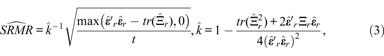
Shi, Maydeu-Olivares and Rosseel (2020) introduced an asymptotically unbiased estimate of the population SRMR in ordinal factor analysis models:

\hat{SRMR} = {\hat{k}}^{- 1} \sqrt{\frac{max ({\hat{ε}'}_{r} {\hat{ε}}_{r} - tr ({\hat{Ξ}}_{r}), 0)}{t}}, \hat{k} = 1 - \frac{tr (\hat{Ξ_{r}^{2}}) + 2 {\hat{ε}'}_{r} Ξ_{r} {\hat{ε}}_{r}}{4 {({\hat{ε}'}_{r} {\hat{ε}}_{r})}^{2}},

(3)

The asymptotic standard error of SRMR is given as follows:

S E_{SRMR} = \sqrt{k^{- 2} \frac{tr (Ξ_{r}^{2}) + 2 {\hat{ε}'}_{r} Ξ_{r} {\hat{ε}}_{r}}{2 t {\hat{ε}'}_{r} {\hat{ε}}_{r}}}

(4)

$Ξ_{r}$ represent the asymptotic covariance matrix of ${\hat{ε}}_{r}$ (see Maydeu-Olivares, 2017a and Shi, Maydeu-Olivares, & Rosseel, 2020 for the computation details for $Ξ_{r}$ ).

Using the ULS estimation method, the population RMSEA under ordinal factor analysis models is defined as follows:

RMSEA = \sqrt{\frac{G}{df}} = \sqrt{\frac{{ε'}_{r} ε_{r}}{df}}

(5)

where $G$ denotes the discrepancy function under ULS estimation. df represents the degrees of freedom for the fitted model. The other notations are the same as defined before. A sample estimate for G can be given as $\hat{G} = φ (r) = \hat{ε}'_{r} \hat{ε_{r}}$ . However, $\hat{G}$ is a biased estimate for G, especially when the sample size is small.

Lai (2020) derived the unbiased sample estimate $({\hat{G}}_{BC})$ and the asymptotic standard error $(S E_{G})$ of G.

{\hat{G}}_{BC} = \hat{G} - \frac{1}{2 n} tr (Q Π)

(6)

S E_{G} = \sqrt{g^{'} Π g}

(7)

Q is the second derivative of $φ (r)$ evaluated at $r = ρ$ . $Π$ is the asymptotic covariance matrix of $\sqrt{n} (r - ρ)$ . $g^{'}$ is the derivative of $φ (r)$ evaluated at $r = ρ$ . More technical details are provided in the work by Lai (2020).

The above formulas can be expanded with multiply imputed data sets. Let m be the number of imputations, and d = 1, 2, . . . m denote a given imputed data set. As a normal sampling distribution is used for SRMR and G, the pooled point estimates and standard errors for SRMR and G (thus RMSEA) across the imputed data sets can be given by applying Rubin’s rules (Rubin, 1976, 1987). Specifically, the unbiased sample MI-based SRMR $({\hat{SRMR}}_{MI})$ and RMSEA $({\hat{RMSEA}}_{MI})$ are computed as follows:

{\hat{SRMR}}_{MI} = \frac{1}{m} \sum_{d = 1}^{m} {\hat{SRMR}}_{d}

(8)

{\hat{RMSEA}}_{MI} = \sqrt{\frac{{\hat{G}}_{MI}}{df}} = \sqrt{(\frac{1}{m} \sum_{d = 1}^{m} {\hat{G}}_{BC} / d f_{d})}

(9)

The pooled standard error can be derived using the within imputation variance $(V_{W})$ and between imputation variance $(V_{B})$ as follows:

S E_{pooled} = \sqrt{V_{W} + V_{B} + \frac{V_{B}}{m}}

(10)

Using Equation 10, the pooled standard error for SRMR $(S E_{SRMR_pooled})$ can be computed with $V_{W} = \frac{1}{m} \sum_{d = 1}^{m} S {E_{SRMR}}_{d}^{2}$ and $V_{B} = (\sum_{d = 1}^{m} ({\hat{SRMR}}_{d} - {\hat{SRMR}}_{MI})^{2}) / (m - 1)$ . Similarly, the pooled standard error for G $(S E_{G_pooled})$ is given by plugging $V_{W} = (1 / m) \sum_{d = 1}^{m} S {E_{G}}_{d}^{2}$ and $V_{B} = (\sum_{d = 1}^{m} {({\hat{G}}_{BC}_{d} - {\hat{G}}_{MI})}^{2}) / (m - 1)$ in Equation 10.

CIs for SRMR and RMSEA under multiply imputed data can be constructed using the pooled unbiased estimates and standard errors. Given an α level, the (100 −α)% CI for the SRMR and RMSEA can be obtained using a reference normal distribution as follows:

[{\hat{SRMR}}_{MI} - z_{α / 2} S E_{SRM R_{pooled}}, {\hat{SRMR}}_{MI} + z_{α / 2} S E_{SRM R_{pooled}}]

(11)

[\sqrt{\frac{({\hat{G}}_{MI} - z_{α / 2} S E_{G_{pooled}})}{df}}, \sqrt{\frac{({\hat{G}}_{MI} + z_{α / 2} S E_{G_{pooled}})}{df}}]

(12)

Simulation Study

Data Generation

A simulation study was conducted to examine the performance of the proposed method for assessing close fit in ordinal factor analysis models with multiply imputed data. We consider ordinal factor analysis models with misspecified dimensionality. That is, the population model had two correlated factors, but a unidimensional model was fitted to the data. For the population model, there were 10 observed variables; each latent factor was measured by five observed variables (i.e., f₁ by X₁–X₅ and f₂ by X₆–X₁₀). The population factor loadings were set to 0.70 and the residual variance for each item was set to 0.51. The population values for the inter-factor correlation were manipulated according to different levels of model misspecification.

Based on the population model, we first generated complete continuous data with a multivariate normal distribution. The continuous data were then discretized to create ordinal categories using a set of threshold values. Finally, we introduced missing values on a subset of items (i.e., X₆–X₁₀) according to different mechanisms and percentages of missingness. We manipulated (a) the level of model misspecification, (b) number of response categories, (c) sample size, (d) mechanism of missingness, and (e) the percentage of missing values.

Level of Model Misspecification

Since the model misspecification was introduced by fitting a one-factor model to two-factor data. The levels of model misspecification were manipulated by altering the population inter-factor correlations (ρ) with four values (i.e., ρ = 0.9, 0.8, 0.7, and 0.6). A smaller value of the correlation coefficients indicates more severe levels of model misspecification.

Sample Size (N)

Levels of sample sizes included 200, 500, and 1,000.

Number of Response Categories (c)

We generated both binary (c = 2) and polytomous data with c = 5 using different sets of threshold values. For binary data (0/1), the population threshold was set to 0, which implied that half of the respondents were expected to provide a response of “1.” When the data had five ordered categories, the four threshold values were −1.28, −0.52, 0.52, and 1.28 such that the expected area under the normal curve was 7%, 24%, 38%, 24%, and 7% for each of the response categories ranging from 0 to 4, respectively. The thresholds used in the current study were consistent with values in previous simulation studies (Forero et al., 2009; Rhemtulla et al., 2012; Shi, Maydeu-Olivares, & Rosseel, 2020).

Mechanism of Missingness

We considered both MCAR and MAR. For MCAR, x% of the observations were randomly selected, and their values on X₆–X₁₀ were removed as missing. Under the mechanism of MAR, the missingness on X₆–X₁₀ was determined by the sum score of Items 1 to 5. That is, if the sum scores for items X₁ through X₅ were greater than the xth percentile, missing values were created by deleting the observations on X₆–X₁₀. The above approach for generating missing data has been utilized in many previous studies (e.g., Shi, Lee, et al., 2020; Shi et al., 2021; Zhang & Wang, 2013).

Percentage of Missing Data

Three levels of percentage of missing data (x%) were studied, including x = 15, 25, and 50. The levels were chosen to represent relatively small, medium, or large proportions of missing data, respectively.

In total, 144 different simulation conditions were included in the study (i.e., 4 levels of model misspecification × 3 levels of sample size × 2 numbers of response categories × 2 mechanisms of missing data × 3 percentages of missing data). For each simulation condition, 1,000 replication datasets were generated using R 4.1.2 (R Core Team, 2020).

Data Analysis

In terms of data analysis, first, the missing values were handled by the MI method. It is noted that several algorithms have been proposed for imputing ordinal missing data (see Jia, 2016, for a review). Based on the recommendations from recent simulation studies (Jia & Wu, 2019), we used the latent variable approach to conduct the imputation. The imputation was conducted using Mplus 8.0 (Muthén & Muthén, 1998–2020) and the number of imputations (m) was set to 100. Then, a one-factor ordinal factor analysis model was fitted to each imputed (completed) data using the ULS estimation method. Finally, for each replication, we obtained the aggregated unbiased sample SRMR and RMSEA values and the 90% CIs across the multiply imputed data using the proposed method. All the data analyses were conducted using the lavaan R package version 0.6-8 (Rosseel, 2012).

To evaluate the performance of the proposed method, for each simulation condition, we obtained the average sample SRMRs and RMSEAs across replications and compared the results with the corresponding population value. In addition, we computed the coverage rate of the 90% CI as the percentage of CIs across replications that include the true population value.

Results

We first computed and reported the population SRMR and RMSEA values across the simulated conditions in Tables 1 and 2. Not surprisingly, for both SRMR and RMSEA, their population values increased as the inter-factor correlations decreased (i.e., the level of model misspecification increased). The population SRMR considered in the current study ranged from 0.022 to 0.088, and the population RMSEA ranged from 0.028 to 0.110. The average MI-based sample SRMR and RMSEA under both MAR and MCAR are also summarized in Tables 1 and 2. The behaviors of sample SRMRs and RMSEAs were very similar across the two missing data mechanisms.

Table 1

Average MI-Based Sample SRMR.

CAT	N	PM	MAR								MCAR
			ρ = 0.90		ρ = 0.80		ρ = 0.70		ρ = 0.60		ρ = 0.90		ρ = 0.80		ρ = 0.70		ρ = 0.60
			POP	SRMR	POP	SRMR	POP	SRMR	POP	SRMR	POP	SRMR	POP	SRMR	POP	SRMR	POP	SRMR
2	200	15	0.022	0.027	0.044	0.049	0.066	0.071	0.088	0.093	0.022	0.035	0.044	0.053	0.066	0.073	0.088	0.093
		25	0.022	0.038	0.044	0.058	0.066	0.078	0.088	0.098	0.022	0.046	0.044	0.061	0.066	0.079	0.088	0.098
		50	0.022	0.080	0.044	0.092	0.066	0.105	0.088	0.119	0.022	0.073	0.044	0.086	0.066	0.099	0.088	0.115
	500	15	0.022	0.025	0.044	0.047	0.066	0.069	0.088	0.092	0.022	0.029	0.044	0.048	0.066	0.069	0.088	0.091
		25	0.022	0.030	0.044	0.051	0.066	0.072	0.088	0.094	0.022	0.035	0.044	0.052	0.066	0.072	0.088	0.093
		50	0.022	0.054	0.044	0.066	0.066	0.084	0.088	0.103	0.022	0.051	0.044	0.064	0.066	0.082	0.088	0.101
	1,000	15	0.022	0.024	0.044	0.046	0.066	0.069	0.088	0.091	0.022	0.026	0.044	0.046	0.066	0.068	0.088	0.090
		25	0.022	0.027	0.044	0.047	0.066	0.069	0.088	0.091	0.022	0.029	0.044	0.048	0.066	0.069	0.088	0.090
		50	0.022	0.038	0.044	0.052	0.066	0.070	0.088	0.091	0.022	0.040	0.044	0.056	0.066	0.075	0.088	0.095
5	200	15	0.022	0.027	0.044	0.048	0.066	0.070	0.088	0.092	0.022	0.028	0.044	0.048	0.066	0.069	0.088	0.091
		25	0.022	0.034	0.044	0.052	0.066	0.074	0.088	0.095	0.022	0.033	0.044	0.052	0.066	0.071	0.088	0.093
		50	0.022	0.051	0.044	0.064	0.066	0.083	0.088	0.102	0.022	0.050	0.044	0.064	0.066	0.081	0.088	0.100
	500	15	0.022	0.025	0.044	0.046	0.066	0.069	0.088	0.090	0.022	0.025	0.044	0.046	0.066	0.068	0.088	0.089
		25	0.022	0.027	0.044	0.047	0.066	0.069	0.088	0.091	0.022	0.027	0.044	0.048	0.066	0.069	0.088	0.090
		50	0.022	0.035	0.044	0.051	0.066	0.070	0.088	0.089	0.022	0.036	0.044	0.053	0.066	0.073	0.088	0.093
	1,000	15	0.022	0.024	0.044	0.045	0.066	0.067	0.088	0.090	0.022	0.024	0.044	0.045	0.066	0.067	0.088	0.089
		25	0.022	0.025	0.044	0.046	0.066	0.068	0.088	0.089	0.022	0.025	0.044	0.046	0.066	0.068	0.088	0.089
		50	0.022	0.029	0.044	0.047	0.066	0.069	0.088	0.090	0.022	0.030	0.044	0.049	0.066	0.070	0.088	0.092

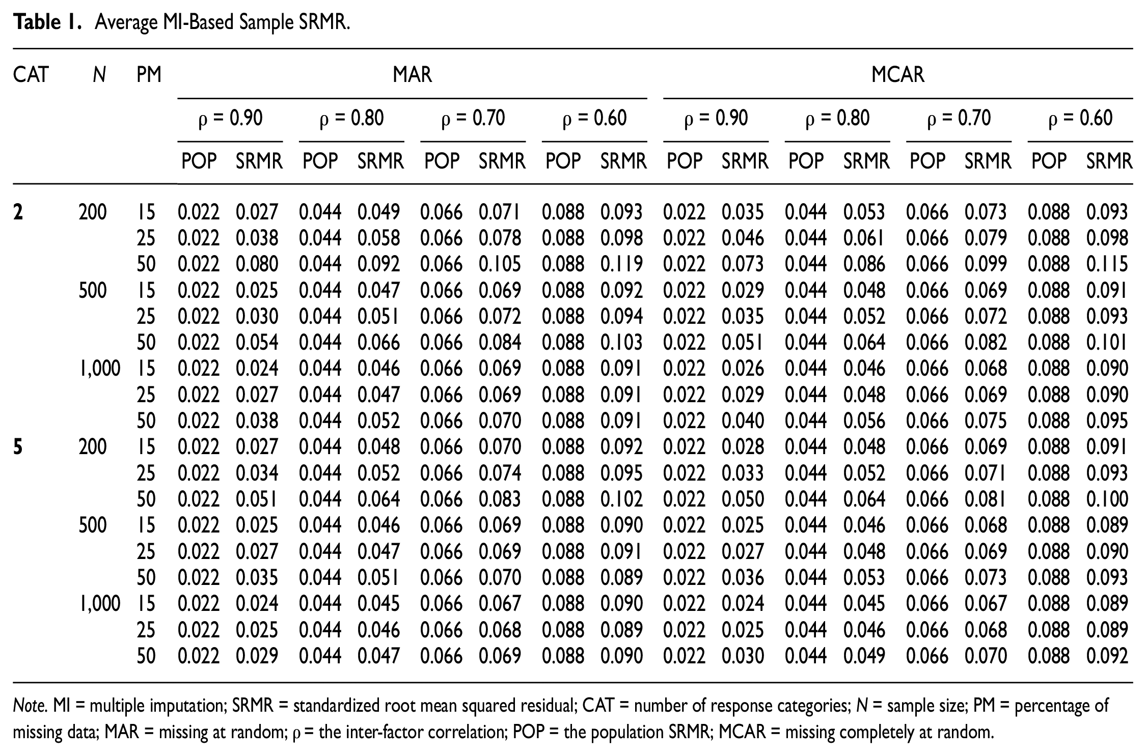
Note. MI = multiple imputation; SRMR = standardized root mean squared residual; CAT = number of response categories; N = sample size; PM = percentage of missing data; MAR = missing at random; ρ = the inter-factor correlation; POP = the population SRMR; MCAR = missing completely at random.

Table 2

Average MI-Based Sample RMSEA.

CAT	N	PM	MAR								MCAR
			ρ = 0.90		ρ = 0.80		ρ = 0.70		ρ = 0.60		ρ = 0.90		ρ = 0.80		ρ = 0.70		ρ = 0.60
			POP	RMSEA	POP	RMSEA	POP	RMSEA	POP	RMSEA	POP	RMSEA	POP	RMSEA	POP	RMSEA	POP	RMSEA
2	200	15	0.028	0.035	0.055	0.062	0.083	0.090	0.110	0.117	0.028	0.045	0.055	0.067	0.083	0.091	0.110	0.117
		25	0.028	0.050	0.055	0.075	0.083	0.100	0.110	0.126	0.028	0.059	0.055	0.078	0.083	0.100	0.110	0.123
		50	0.028	0.103	0.055	0.119	0.083	0.136	0.110	0.154	0.028	0.093	0.055	0.108	0.083	0.125	0.110	0.146
	500	15	0.028	0.032	0.055	0.059	0.083	0.087	0.110	0.115	0.028	0.036	0.055	0.061	0.083	0.087	0.110	0.113
		25	0.028	0.039	0.055	0.064	0.083	0.090	0.110	0.118	0.028	0.044	0.055	0.065	0.083	0.091	0.110	0.116
		50	0.028	0.069	0.055	0.085	0.083	0.108	0.110	0.132	0.028	0.064	0.055	0.081	0.083	0.103	0.110	0.127
	1,000	15	0.028	0.030	0.055	0.058	0.083	0.086	0.110	0.114	0.028	0.033	0.055	0.058	0.083	0.085	0.110	0.112
		25	0.028	0.034	0.055	0.059	0.083	0.087	0.110	0.115	0.028	0.036	0.055	0.060	0.083	0.086	0.110	0.113
		50	0.028	0.049	0.055	0.066	0.083	0.090	0.110	0.116	0.028	0.050	0.055	0.070	0.083	0.094	0.110	0.120
5	200	15	0.028	0.036	0.055	0.061	0.083	0.088	0.110	0.115	0.028	0.036	0.055	0.061	0.083	0.087	0.110	0.114
		25	0.028	0.044	0.055	0.067	0.083	0.094	0.110	0.120	0.028	0.043	0.055	0.065	0.083	0.090	0.110	0.116
		50	0.028	0.066	0.055	0.083	0.083	0.107	0.110	0.131	0.028	0.064	0.055	0.082	0.083	0.103	0.110	0.126
	500	15	0.028	0.031	0.055	0.058	0.083	0.086	0.110	0.113	0.028	0.031	0.055	0.057	0.083	0.084	0.110	0.112
		25	0.028	0.035	0.055	0.060	0.083	0.087	0.110	0.114	0.028	0.034	0.055	0.060	0.083	0.086	0.110	0.113
		50	0.028	0.045	0.055	0.065	0.083	0.089	0.110	0.113	0.028	0.045	0.055	0.067	0.083	0.091	0.110	0.117
	1,000	15	0.028	0.030	0.055	0.057	0.083	0.085	0.110	0.112	0.028	0.029	0.055	0.056	0.083	0.084	0.110	0.111
		25	0.028	0.031	0.055	0.057	0.083	0.085	0.110	0.112	0.028	0.031	0.055	0.058	0.083	0.085	0.110	0.112
		50	0.028	0.037	0.055	0.060	0.083	0.087	0.110	0.113	0.028	0.038	0.055	0.061	0.083	0.088	0.110	0.115

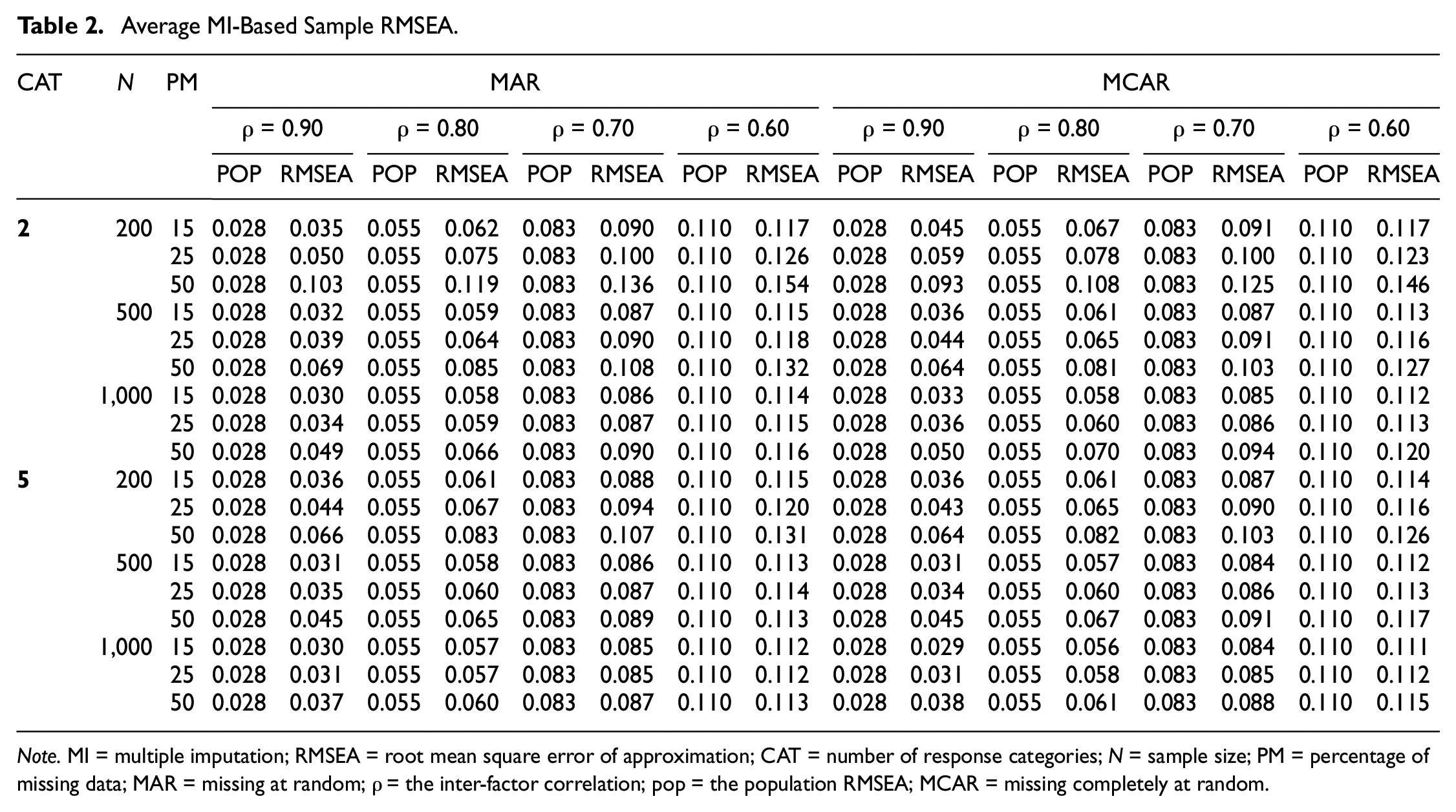
Note. MI = multiple imputation; RMSEA = root mean square error of approximation; CAT = number of response categories; N = sample size; PM = percentage of missing data; MAR = missing at random; ρ = the inter-factor correlation; pop = the population RMSEA; MCAR = missing completely at random.

As shown in Table 1, in the presence of missing data, the MI-based SRMRs could be overestimated, suggesting worse model fit compared with their population values. The bias of the MI-based SRMR² increased as the sample size decreased, the percentage of missing data increased, and the number of response categories decreased. For example, when ρ = 0.8, N = 1,000, the number of response categories was 5 and 15% of the observations were MAR; the average value for ${\hat{SRMR}}_{MI}$ (0.045) was very close to the population value (0.044). However, as the sample size (N) decreased to 200, the number of response categories (c) decreased to 2, and the percentage of missing data increased to 50%, the average sample estimate for ${\hat{SRMR}}_{MI}$ was noticeably inflated to 0.086.

Similar patterns were observed for the MI-based sample RMSEA $({\hat{RMSEA}}_{MI})$ . As shown in Table 2, the average ${\hat{RMSEA}}_{MI}$ became closer to its population value as sample size increased, the percentage of missingness decreased and the number of response categories increased. For example, when ρ = 0.7, N = 1,000, the number of response categories was 5 and 15% of the observations were MCAR; the average ${\hat{RMSEA}}_{MI} = 0.084$ , which is very close the population RMSEA = 0.083. As sample size decreased to 200 and percentage of missingness increased to 50% and everything else was held constant, the MI-based sample RMSEA tended to be overestimated, with average ${\hat{RMSEA}}_{MI} = 0.103$ .

We summarized the coverage rates of the 90% CIs around the population SRMR and RMSEA across simulated conditions in Tables 3 and 4, respectively. Coverage rates greater than 80% (i.e., 90% ± 10%) are highlighted in bold. Results indicated that for SRMR, regardless of the mechanism of missing data, the CIs were more accurate as the sample size (N) increased, the percentage of missing data decreased, the number of response categories (c) increased, and the level of model misspecification became more severe. For example, as shown in Table 3, under MAR, when N = 200, c = 2, ρ = 0.90, and 25% of the observations were missing, the coverage rate for the 90% CIs was 79%. The coverage rate improved to 89% under conditions of N = 1,000, c = 5, ρ = 0.60, and missing percentage = 15%.

Table 3

Coverage Rates (CRs) of the 90% Confidence Intervals: SRMR.

CAT	N	PM	MAR								MCAR
			ρ = 0.90		ρ = 0.80		ρ = 0.70		ρ = 0.60		ρ = 0.90		ρ = 0.80		ρ = 0.70		ρ = 0.60
			POP	CR	POP	CR	POP	CR	POP	CR	POP	CR	POP	CR	POP	CR	POP	CR
2	200	15	0.022	0.87	0.044	0.86	0.066	0.87	0.088	0.88	0.022	0.75	0.044	0.84	0.066	0.87	0.088	0.87
		25	0.022	0.79	0.044	0.86	0.066	0.89	0.088	0.90	0.022	0.57	0.044	0.77	0.066	0.86	0.088	0.88
		50	0.022	0.14	0.044	0.53	0.066	0.73	0.088	0.80	0.022	0.06	0.044	0.27	0.066	0.58	0.088	0.76
	500	15	0.022	0.81	0.044	0.90	0.066	0.87	0.088	0.89	0.022	0.78	0.044	0.87	0.066	0.88	0.088	0.88
		25	0.022	0.78	0.044	0.87	0.066	0.88	0.088	0.87	0.022	0.64	0.044	0.83	0.066	0.85	0.088	0.89
		50	0.022	0.21	0.044	0.75	0.066	0.84	0.088	0.86	0.022	0.07	0.044	0.47	0.066	0.74	0.088	0.84
	1,000	15	0.022	0.88	0.044	0.87	0.066	0.89	0.088	0.89	0.022	0.82	0.044	0.88	0.066	0.89	0.088	0.90
		25	0.022	0.85	0.044	0.90	0.066	0.89	0.088	0.91	0.022	0.73	0.044	0.87	0.066	0.89	0.088	0.89
		50	0.022	0.55	0.044	0.93	0.066	0.95	0.088	0.93	0.022	0.19	0.044	0.66	0.066	0.82	0.088	0.85
5	200	15	0.022	0.86	0.044	0.91	0.066	0.91	0.088	0.91	0.022	0.82	0.044	0.88	0.066	0.89	0.088	0.91
		25	0.022	0.76	0.044	0.90	0.066	0.88	0.088	0.89	0.022	0.70	0.044	0.87	0.066	0.90	0.088	0.91
		50	0.022	0.26	0.044	0.79	0.066	0.88	0.088	0.89	0.022	0.14	0.044	0.60	0.066	0.83	0.088	0.88
	500	15	0.022	0.87	0.044	0.88	0.066	0.90	0.088	0.89	0.022	0.86	0.044	0.88	0.066	0.89	0.088	0.90
		25	0.022	0.81	0.044	0.87	0.066	0.89	0.088	0.86	0.022	0.82	0.044	0.86	0.066	0.88	0.088	0.88
		50	0.022	0.56	0.044	0.90	0.066	0.93	0.088	0.91	0.022	0.34	0.044	0.75	0.066	0.85	0.088	0.88
	1,000	15	0.022	0.88	0.044	0.87	0.066	0.88	0.088	0.89	0.022	0.87	0.044	0.89	0.066	0.88	0.088	0.88
		25	0.022	0.88	0.044	0.91	0.066	0.92	0.088	0.92	0.022	0.83	0.044	0.86	0.066	0.89	0.088	0.90
		50	0.022	0.68	0.044	0.88	0.066	0.90	0.088	0.91	0.022	0.49	0.044	0.80	0.066	0.86	0.088	0.89

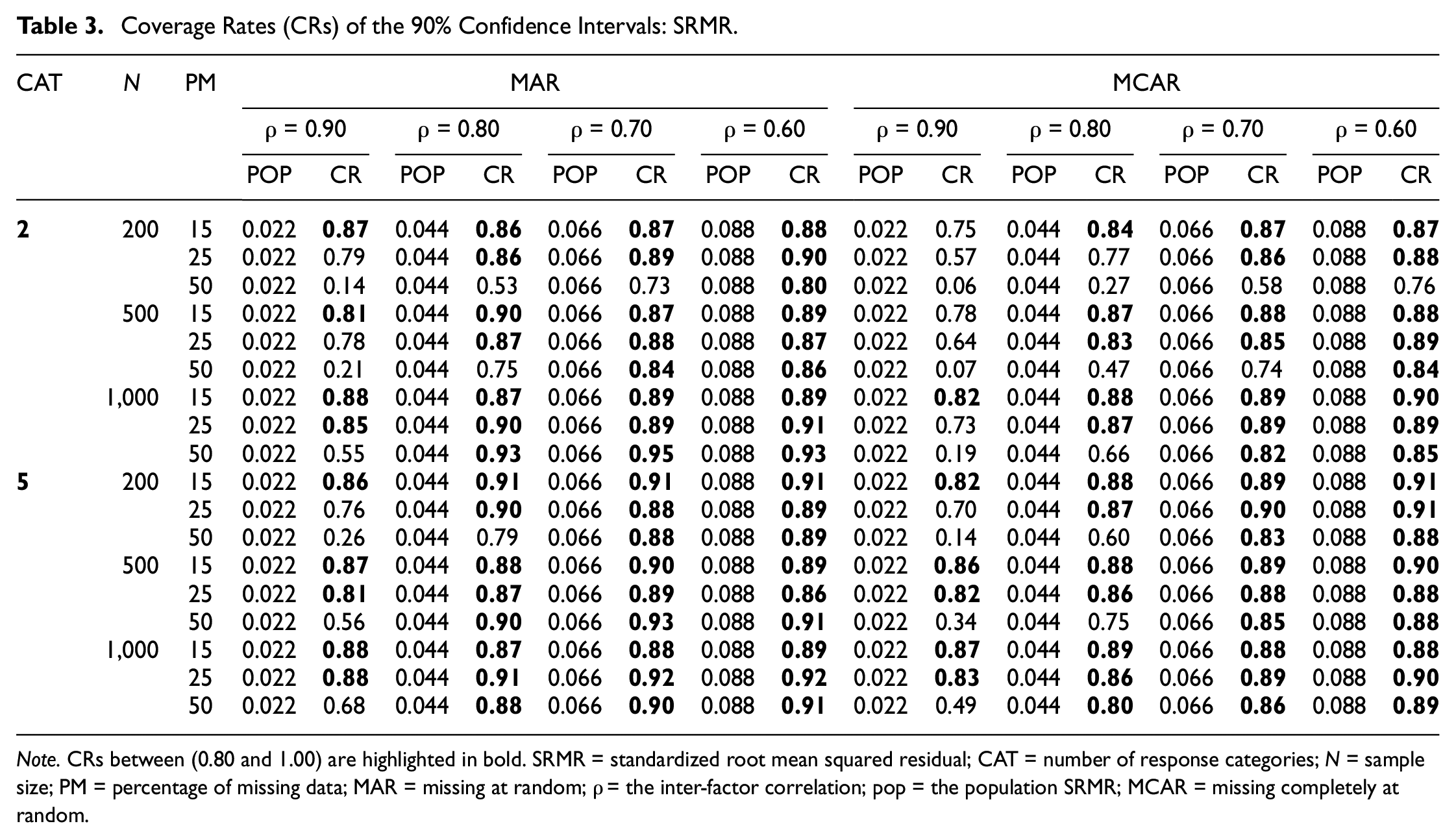
Note. CRs between (0.80 and 1.00) are highlighted in bold. SRMR = standardized root mean squared residual; CAT = number of response categories; N = sample size; PM = percentage of missing data; MAR = missing at random; ρ = the inter-factor correlation; pop = the population SRMR; MCAR = missing completely at random.

Table 4

Coverage Rates (CRs) of the 90% Confidence Intervals: RMSEA.

CAT	N	PM	MAR								MCAR
			ρ = 0.90		ρ = 0.80		ρ = 0.70		ρ = 0.60		ρ = 0.90		ρ = 0.80		ρ = 0.70		ρ = 0.60
			POP	CR	POP	CR	POP	CR	POP	CR	POP	CR	POP	CR	POP	CR	POP	CR
2	200	15	0.028	0.98	0.055	0.96	0.083	0.93	0.110	0.91	0.028	0.98	0.055	0.97	0.083	0.95	0.110	0.92
		25	0.028	0.98	0.055	0.97	0.083	0.96	0.110	0.94	0.028	0.93	0.055	0.93	0.083	0.96	0.110	0.93
		50	0.028	0.71	0.055	0.84	0.083	0.89	0.110	0.90	0.028	0.46	0.055	0.62	0.083	0.78	0.110	0.87
	500	15	0.028	0.98	0.055	0.96	0.083	0.93	0.110	0.93	0.028	0.97	0.055	0.96	0.083	0.92	0.110	0.91
		25	0.028	0.94	0.055	0.92	0.083	0.90	0.110	0.88	0.028	0.90	0.055	0.93	0.083	0.92	0.110	0.91
		50	0.028	0.74	0.055	0.92	0.083	0.94	0.110	0.91	0.028	0.40	0.055	0.72	0.083	0.87	0.110	0.91
	1,000	15	0.028	0.95	0.055	0.91	0.083	0.90	0.110	0.90	0.028	0.95	0.055	0.93	0.083	0.90	0.110	0.92
		25	0.028	0.96	0.055	0.91	0.083	0.90	0.110	0.91	0.028	0.91	0.055	0.92	0.083	0.92	0.110	0.91
		50	0.028	0.87	0.055	0.97	0.083	0.96	0.110	0.94	0.028	0.49	0.055	0.80	0.083	0.88	0.110	0.90
5	200	15	0.028	0.97	0.055	0.94	0.083	0.92	0.110	0.92	0.028	0.97	0.055	0.94	0.083	0.92	0.110	0.91
		25	0.028	0.95	0.055	0.96	0.083	0.93	0.110	0.93	0.028	0.95	0.055	0.97	0.083	0.96	0.110	0.94
		50	0.028	0.76	0.055	0.95	0.083	0.96	0.110	0.93	0.028	0.46	0.055	0.77	0.083	0.91	0.110	0.92
	500	15	0.028	0.93	0.055	0.88	0.083	0.89	0.110	0.88	0.028	0.93	0.055	0.89	0.083	0.89	0.110	0.89
		25	0.028	0.94	0.055	0.91	0.083	0.91	0.110	0.88	0.028	0.93	0.055	0.92	0.083	0.91	0.110	0.90
		50	0.028	0.88	0.055	0.96	0.083	0.95	0.110	0.92	0.028	0.53	0.055	0.81	0.083	0.88	0.110	0.89
	1,000	15	0.028	0.95	0.055	0.92	0.083	0.92	0.110	0.91	0.028	0.94	0.055	0.91	0.083	0.89	0.110	0.89
		25	0.028	0.93	0.055	0.92	0.083	0.92	0.110	0.92	0.028	0.90	0.055	0.88	0.083	0.89	0.110	0.89
		50	0.028	0.83	0.055	0.92	0.083	0.92	0.110	0.92	0.028	0.65	0.055	0.83	0.083	0.88	0.110	0.90

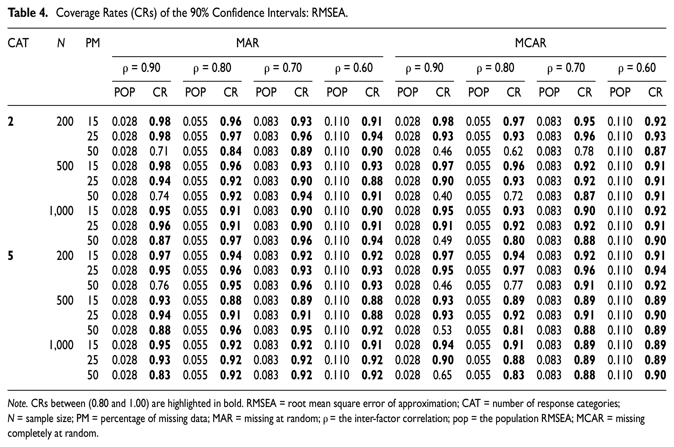
Note. CRs between (0.80 and 1.00) are highlighted in bold. RMSEA = root mean square error of approximation; CAT = number of response categories; N = sample size; PM = percentage of missing data; MAR = missing at random; ρ = the inter-factor correlation; pop = the population RMSEA; MCAR = missing completely at random.

As shown in Table 4, the CIs for RMSEA exhibited very similar behaviors. Across all simulated conditions considered in this study, the CI coverage rates were close to the 90% nominal levels, except for when models with minor levels of misspecification were fit to a small sample with a large proportion of missing data. It is noted that under the undesirable conditions mentioned above, the CIs for RMSEA yielded more accurate coverage rates than the CIs obtained from SRMR. For example, when N = 200, c = 2, ρ = 0.90, and 50% of the observations were MAR, the 90% CI coverage rates for RMSEA and SRMR were 71% and 14%, respectively.

Discussion

Major Findings and Recommendations

In this study, we proposed methods for assessing close fit in ordinal factor analysis models under missing data. Specifically, for both SRMR and RMSEA, we introduced the procedure for computing the MI-based sample estimates and constructing the CIs with multiply imputed data. The performance of the proposed method was evaluated using a simulation study across different sample sizes, numbers of response categories, levels of model misspecification, mechanisms of missingness, and percentages of missing data.

Results showed that with multiply imputed data, the sample SRMR $({\hat{SRMR}}_{MI})$ and RMSEA $({\hat{RMSEA}}_{MI})$ approached their population values as sample size increased and the percentage of missingness decreased. In addition, for both SRMR and RMSEA, the proposed CIs could yield relatively accurate coverage rates across the simulated conditions, except for conditions with a large proportion of missing data (e.g., ≥50%) and/or with a minor level of model misfit (e.g., population SRMR = 0.022 or population RMSEA = 0.028).

The above results were consistent with previous findings with complete data reported in the work by Shi, Maydeu-Olivares and Rosseel (2020); the authors also found that the CI for SRMR tended to be less accurate when the level of model misfit became more minor. It is noted that though poor CI coverage rates could be observed under models with a minor level of misfit (i.e., ρ = 0.90), the average MI-based SRMR and RMSEA values still tended to be below the conventional cutoffs for acceptable fit (Hu & Bentler, 1999), except when the percentage of missing data reached 50%.

From an applied perspective, the current study provided implications for researchers who work with ordinal factor analysis models with missing data. The MI method has been recommended by previous studies for handling missing data in ordinal factor analysis models (e.g., Asparouhov & Muthén, 2010b; Shi, Maydeu-Olivares, & Rosseel, 2020). By using the procedures introduced in the current article, both SRMR and RMSEA could be used for assessing the fit of ordinal factor analysis with multiply imputed data. Based on our findings, we recommend researcher to report the unbiased MI-based SRMR $({\hat{SRMR}}_{MI})$ and RMSEA $({\hat{RMSEA}}_{MI})$ with their CIs. Researchers should be cautious in interpreting the model fit results when the percentage of missing data reaches 50%, especially when the sample size is small (e.g., N≤ 200) and the number of response categories is small (c = 2). Under the above conditions, both SRMR and RMSEA tended to yield sample estimates that suggested a worse fit than their population values. In addition, when evaluating models with minor misspecifications, and/or with a large percentage of missing data (e.g., 50%), the CIs for RMSEA are more trustworthy than those obtained from SRMR. In the next section, we presented an empirical example to illustrate the proposed method for assessing the fit of ordinal factor analysis models with missing data.

An Empirical Example

We used part of the large data set from the National Longitudinal Survey of Youth 1979—Child and Young Adult Cohort (NLSY79-CYA, U.S. Department of Labor, U.S. Bureau of Labor Statistics, and National Institute of Child Health and Human Development, 2019). The latent variable of interest is the depression symptoms measured by the Center for Epidemiologic Studies Depression Scale (CES-D; Radloff, 1977). The original CES-D includes 20 items (e.g., I felt depressed) asking the respondents to rate how often over the past 7 days they experienced depression symptoms using a Likert-type scale ranging from 0 (rarely or none of the time) to 3 (most or almost all the time). A shorter, 7-item version of the CES-D scale was used in NLSY-CYA. The CES-D data collected in the waves of 2004 and 2008 were used in the analysis. For the purpose of demonstration, we randomly selected 1,000 observations from the sample; 700 participants responded to the CES-D scale at both waves, and 300 individuals only provided responses to the CES-D scale at the first wave (i.e., 2004). The empirical example reflected the scenario in longitudinal studies with a 30% attrition rate, and closely matched the conditions considered in our simulation study (i.e., p = 14 observed variables, 30% of missing data, and sample size N = 1,000).

We fitted a longitudinal ordinal factor analysis model to the data. Specifically, a unidimensional ordinal confirmatory factor analysis (CFA) model was assumed on each time occasion. The latent factors (i.e., depression) and the error terms for the same item were allowed to be correlated across time. All the model parameters, other than those for model identification purposes, were freely estimated. To handle missing data, we first conducted MI using the latent variable approach with a number of imputations, m = 100. Then, an ordinal factor analysis model was fitted to each imputed data using the ULS estimation method. Using the procedure introduced in the current article, for both SRMR and RMSEA, we aggregated and computed their sample estimates and the corresponding CIs. The imputation was conducted using Mplus (Muthén & Muthén, 1998–2017), and the data analysis and pooling were conducted using the lavaan R package.

Results showed that the MI-based SRMR $({\hat{SRMR}}_{MI})$ was 0.048, with a 90% CI = [0.039, 0.056]. The MI-based RMSEA $({\hat{RMSEA}}_{MI})$ was 0.058, with a 90% CI = [0.048, 0.068]. Based on the results from the simulation study, for both SRMR and RMSEA, the MI-based sample estimates and CIs are expected to be trustworthy.

Limitations and Future Directions

This study is not without limitations. First, although we included a large number of conditions (i.e., 144) in the current simulation study, there are other factors we did not manipulate in our simulation design. For example, we only considered one type of model misspecification (i.e., misspecified dimensionality). The performance of the proposed method under other types of model misspecifications (e.g., omitted cross-loading) should be investigated in future studies. In addition, the proposed method only focused on two of the fit indices (i.e., SRMR and RMSEA). Given that evaluating model fit is not an easy task and there is no “golden rule” (Marsh et al., 2004), future studies are expected to develop methods to compute other fit indices (e.g., CFI) for assessing ordinal factor analysis models with multiply imputed data.

Footnotes

Declaration of Conflicting Interests

The authors declared no potential conflicts of interest with respect to the research, authorship, and/or publication of this article.

Funding

The authors received no financial support for the research, authorship, and/or publication of this article.

ORCID iDs

Dexin Shi

Bo Zhang

Ren Liu

Notes

References

Allison

P. D.

(1987). Estimation of linear models with incomplete data. Sociological Methodology, 17(1), 71–103.

Arbuckle

J. L.

(1996). Full information estimation in the presence of incomplete data. In Marcoulides

G. A.

Schumaker

R. E.

(Eds.), Advanced structural equation modeling (pp. 243–277). Lawrence Erlbaum.

Asparouhov

Muthén

(2010a). Multiple imputation with Mplus: Technical implementation. http://statmodel2.com/download/Imputations7.pdf

Asparouhov

Muthén

(2010b). Weighted least squares estimation with missing data: Technical implementation. https://www.statmodel.com/download/GstrucMissingRevision.pdf

Baker

F. B.

Kim

S. H.

(2004). Item response theory: Parameter estimation techniques. CRC Press.

Bentler

P. M.

(1990). Comparative fit indexes in structural models. Psychological Bulletin, 107(2), 238–246.

Bentler

P. M.

Bonett

D. G.

(1980). Significance tests and goodness of fit in the analysis of covariance structures. Psychological Bulletin, 88(3), 588–606.

Brosseau-Liard

P. E.

Savalei

(2014). Adjusting incremental fit indices for nonnormality. Multivariate Behavioral Research, 49(5), 460–470.

Enders

C. K.

(2010). Applied missing data analysis. Guilford Press.

10.

Finkbeiner

(1979). Estimation for the multiple factor model when data are missing. Psychometrika, 44(4), 409–420.

11.

Forero

C. G.

Maydeu-Olivares

(2009). Estimation of IRT graded response models: Limited versus full information methods. Psychological Methods, 14(3), 275–299.

12.

Forero

C. G.

Maydeu-Olivares

Gallardo-Pujol

(2009). Factor analysis with ordinal indicators: A Monte Carlo study comparing DWLS and ULS estimation. Structural Equation Modeling, 16(4), 625–641.

13.

L. T.

Bentler

P. M.

(1999). Cutoff criteria for fit indexes in covariance structure analysis: Conventional criteria versus new alternatives. Structural Equation Modeling, 6(1), 1–55.

14.

Jia

(2016). Methods for handling missing non-normal data in structural equation modeling [Doctoral dissertation, The University of Kansas].

15.

Jia

(2019). Evaluating methods for handling missing ordinal data in structural equation modeling. Behavior Research Methods, 51(5), 2337–2355.

16.

Jöreskog

K. G

. (1969). A general approach to confirmatory maximum likelihood factor analysis. Psychometrika, 34, 183–202. https://doi.org/10.1007/BF02289343

17.

Jöreskog

K. G.

Sörbom

(1988). LISREL 7. A guide to the program and applications (2nd ed.). International Education Services.

18.

Kamata

Bauer

D. J.

(2008). A note on the relation between factor analytic and item response theory models. Structural Equation Modeling, 15(1), 136–153.

19.

Lai

(2020). Correct point estimator and confidence interval for RMSEA given categorical data. Structural Equation Modeling, 27(5), 678–695.

20.

Likert

(1932). A technique for the measurement of attitudes. Archives of Psychology, 140, 44–53.

21.

Marsh

H. W.

Hau

K. T.

Wen

(2004). In search of golden rules: Comment on hypothesis-testing approaches to setting cutoff values for fit indexes and dangers in overgeneralizing Hu and Bentler’s (1999) findings. Structural Equation Modeling, 11(3), 320–341.

22.

Maydeu-Olivares

(2017a). Assessing the size of model misfit in structural equation models. Psychometrika, 82(3), 533–558.

23.

Maydeu-Olivares

(2017b). Maximum likelihood estimation of structural equation models for continuous data: Standard errors and goodness of fit. Structural Equation Modeling, 24(3), 383–394.

24.

Maydeu-Olivares

Joe

(2005). Limited-and full-information estimation and goodness-of-fit testing in 2n contingency tables: A unified framework. Journal of the American Statistical Association, 100(471), 1009–1020.

25.

Muthén

(1993). Goodness of fit with categorical and other nonnormal variables. In Bollen

K. A.

Long

J. S.

(Eds.), Testing structural equation models (pp. 205–234). SAGE.

26.

Muthén

B. O.

du Toit

S. H. C.

Spisic

(1997). Robust inference using weighted least squares and quadratic estimating equations in latent variable modeling with categorical and continuous outcomes. http://pages.gseis.ucla.edu/faculty/muthen/articles/Article_075.pdf

27.

Muthén

L. K.

Muthén

B. O.

(1998–2011). Mplus user’s guide (6th ed.).

28.

Peng

C. Y. J.

Harwell

Liou

S. M.

Ehman

L. H.

(2006). Advances in missing data methods and implications for educational research. In Sawilowsky

(Ed.), Real data analysis (pp. 31–78). Information Age.

29.

R Core Team. (2020). R: A language and environment for statistical computing. R Foundation for Statistical Computing. http://www.R-project.org/

30.

Radloff

L. S.

(1977). The CES-D scale: A self-report depression scale for research in the general population. Applied Psychological Measurement, 1(3), 385–401.

31.

Rhemtulla

Brosseau-Liard

P. É. E.

Savalei

(2012). When can categorical variables be treated as continuous? A comparison of robust continuous and categorical SEM estimation methods under suboptimal conditions. Psychological Methods, 17(3), 354–373.

32.

Rosseel

(2012). lavaan: An R package for structural equation modeling. Journal of Statistical Software, 48(2), 1–36.

33.

Rubin

D. B.

(1976). Inference and missing data. Biometrika, 63(3), 581–592.

34.

Rubin

D. B.

(1987). Multiple imputation for nonresponse in surveys. John Wiley.

35.

Saris

W. E.

Satorra

van der Veld

W. M.

(2009). Testing structural equation models or detection of misspecifications? Structural Equation Modeling, 16(4), 561–582.

36.

Savalei

(2017, October). Reconstructing fit indices in SEM with categorical data: Borrowing insights from nonnormal data [Paper presentation]. Annual Meeting of the Society of Multivariate Experimental Psychology, Minneapolis, MN, United States.

37.

Savalei

(2021). Improving fit indices in structural equation modeling with categorical data. Multivariate Behavioral Research, 56(3), 390–407.

38.

Shi

DiStefano

Zheng

Liu

Jiang

(2021). Fitting latent growth models with small sample sizes and non-normal missing data. International Journal of Behavioral Development, 45(2), 179–192.

39.

Shi

Lee

Fairchild

A. J.

Maydeu-Olivares

(2020). Fitting ordinal factor analysis models with missing data: A comparison between pairwise deletion and multiple imputation. Educational and Psychological Measurement, 80(1), 41–66.

40.

Shi

Maydeu-Olivares

(2020). The effect of estimation methods on SEM fit indices. Educational and Psychological Measurement, 80(3), 421–445.

41.

Shi

Maydeu-Olivares

Rosseel

(2020). Assessing fit in ordinal factor analysis models: SRMR vs. RMSEA. Structural Equation Modeling, 27, 1–15.

42.

Steiger

Lind

J. C.

(1980, May). Statistically based tests for the number of common factors[Paper presentation]. Annual Meeting of the Annual Spring Meeting of the Psychometric Society, Iowa City, IA, United States.

43.

Tucker

L. R.

Lewis

(1973). A reliability coefficient for maximum likelihood factor analysis. Psychometrika, 38(1), 1–10.

44.

U.S. Department of Labor, U.S. Bureau of Labor Statistics, and National Institute of Child Health and Human Development. (2019). Children of the NLSY79, 1979-2016. Center for Human Resource Research (CHRR), The Ohio State University.

45.

Xia

(2016). Investigating the chi-square-based model-fit indexes for WLSMV and ULSMV estimators [Unpublished doctoral dissertation, Florida State University].

46.

Xia

Yang

(2019). RMSEA, CFI, and TLI in structural equation modeling with ordered categorical data: The story they tell depends on the estimation methods. Behavior Research Methods, 51(1), 409–428.

47.

Zhang

Wang

(2013). Methods for mediation analysis with missing data. Psychometrika, 78(1), 154–184.

48.

Zyphur

M. J.

Bonner

C. V.

Tay

(2023). Structural equation modeling in organizational research: The state of our science and some proposals for its future. Annual Review of Organizational Psychology and Organizational Behavior, 10, 495–517.

Evaluating Close Fit in Ordinal Factor Analysis Models With Multiply Imputed Data

Abstract

Keywords

Estimating SRMR and RMSEA in Ordinal Factor Analysis Models With Multiply Imputed Data

Simulation Study

Data Generation

Level of Model Misspecification

Sample Size (N)

Number of Response Categories (c)

Mechanism of Missingness

Percentage of Missing Data

Data Analysis

Results

Discussion

Major Findings and Recommendations

An Empirical Example

Limitations and Future Directions

Footnotes

Declaration of Conflicting Interests

Funding

ORCID iDs

Notes

References