A Multidimensional Item Response Theory Model for Continuous and Graded Responses With Error in Persons and Items

Abstract

Item response theory “dual” models (DMs) in which both items and individuals are viewed as sources of differential measurement error so far have been proposed only for unidimensional measures. This article proposes two multidimensional extensions of existing DMs: the M-DTCRM (dual Thurstonian continuous response model), intended for (approximately) continuous responses, and the M-DTGRM (dual Thurstonian graded response model), intended for ordered-categorical responses (including binary). A rationale for the extension to the multiple-content-dimensions case, which is based on the concept of the multidimensional location index, is first proposed and discussed. Then, the models are described using both the factor-analytic and the item response theory parameterizations. Procedures for (a) calibrating the items, (b) scoring individuals, (c) assessing model appropriateness, and (d) assessing measurement precision are finally discussed. The simulation results suggest that the proposal is quite feasible, and an illustrative example based on personality data is also provided. The proposals are submitted to be of particular interest for the case of multidimensional questionnaires in which the number of items per scale would not be enough for arriving at stable estimates if the existing unidimensional DMs were fitted on a separate-scale basis.

A line of psychometric thought that can be traced back to the 1940s considers that “dual” models (DMs; see Ferrando, 2019, and Fiske, 1968) in which both persons and items are sources of measurement error are the most plausible for personality measurement (e.g., Ferrando, 2019; Fiske, 1968; Guilford, 1959). Furthermore, proponents of this view generally consider that the amount of error varies over both respondents and items (see Lumsden, 1980), which agrees with experience. On the one hand, personality items generally vary in their discriminating power (Reise & Waller, 2009), and these variations possibly reflect the degree of item ambiguity as well as such characteristics as type of stem and average item length (e.g., Ferrando, 2013; Lumsden, 1980; Taylor, 1977). On the other hand, individuals generally differ in the sensitivity of their responses to the different item locations (Ferrando, 2013; Fiske, 1968; Guilford, 1959), and this variation is thought to mainly reflect the relevance, degree of clarity, and strength with which the trait is internally organized in the individual (e.g., LaHuis et al., 2017).

A DM fits naturally in a unidimensional item response theory (IRT) framework. The item response can then be viewed as the momentary encounter between an individual, who has a certain trait level, and an item which has a location on the same trait continuum (Lumsden, 1980; Torgerson, 1958), so that, at the moment of responding, the respondent compares his or her perceived momentary level (subject to error) to the perceived item location (also subject to error) on the same continuum. In spite of the simplicity of this mechanism, however, IRT-based attempts to formalize and develop it are relatively recent, and start with the seminal works by Weiss (1973), Levine and Rubin (1979) and, particularly, Strandmark and Linn (1987). Between then and now, the existing proposals have used different parameterizations, response mechanisms, and terminology, and have generally considered restricted versions of the general model outlined above (see Ferrando, 2019). A general, fully workable framework for modeling responses with different amounts of error in both persons and items has been proposed by Ferrando (2013, 2019), and is the basis for the developments proposed here.

To the best of our knowledge all the IRT-based DMs proposed so far are intended for measures of a single content variable, and, in principle, we do not see this restriction as a shortcoming. First, the response mechanism above is quite clear in this context. Second, scores derived from a unidimensional (or essentially unidimensional) instrument are the most univocal, meaningful, and clear to interpret (McDonald, 2000). Multidimensional extensions of the existing proposals, however, are of interest for at least two reasons. First, most personality measures are inherently multidimensional, so that more than one content dimension is needed to understand what their items measure (e.g., Cattell & Tsujioka, 1964). Second, accurate estimation of the person parameter that models the amount of individual error generally requires relatively long tests. So, although a DM can be fitted to multidimensional personality measures on a separate-scale basis, the number of items per scale is generally not large enough to arrive at stable estimates.

The aim of this article is to extend the general modeling framework proposed by Ferrando (2013, 2019) to the case of item sets intended to measure multiple dimensions. The spirit of the proposal is mainly applied, and feasible, simple, and robust procedures are proposed for (a) calibrating the items and assessing model–data fit and appropriateness, (b) estimating the person parameters (scoring), and (c) assessing the precision with which the individual parameters are estimated. As far as we know, the proposal as a whole is a new contribution.

The remainder of the article is as follows: (a) the existing unidimensional DMs intended for continuous and graded-responses dual Thurstonian continuous response model (DTCRM) and the dual Thurstonian graded response model (DTGRM; see Ferrando, 2019; including binary) are revised; (b) the proposed multidimensional extensions of these models, M-DTCRM and MDGRM, are developed in detail; (c) two-stage (calibration and scoring) procedures for fitting the models and assessing their appropriateness are then described; (d) their behavior is assessed with simulation studies; and (e) they are implemented in an extended R package; and finally (f) the functioning of the proposal is illustrated with an empirical example in the personality domain.

A Review of the Unidimensional DTCRM and DTGRM

For item scores that can be treated as (approximately) continuous, the structural equation of the DTCRM is

$$X_{\mathrm{ij}}=\gamma +{\lambda }_j(T_i-b_j).$$

(1)

where X_ij is the score of individual i on item j, γ is the response scale midpoint, and λ_j is a scaling parameter that relates the item score scale to the latent scale of θ. Ti is the momentary trait (or perceived trait) value of this individual at the moment of responding, and bj is the momentary (perceived) location of item j on the trait continuum:

$$T_i={\theta }_i+{\omega }_i;b_j={\beta }_j+{\epsilon }_j.$$

(2)

The distribution of T_i over the test items is assumed to be normal with mean θ_i and variance ${\sigma }_i^2$ , which are the parameters that characterize respondent i, and that remain constant across items. The distribution of b_j, over respondents is assumed to be normal, with mean β _j , and variance ${\sigma }_{{\epsilon }_j}^2$ . Finally, the item and person residuals are assumed to be independent (e.g., Torgerson, 1958). As for interpretation, θ_i (person location), is the single value that best summarizes the standing of individual i on the trait, whereas β _j (item location) can be interpreted as a conventional IRT item location index (see below). The square roots of the variance terms, ${\sigma }_i^2$ and ${\sigma }_{{\epsilon }_j}^2$ (i.e., the σ_i and ${\sigma }_{{\epsilon }_j}$ standard deviations) are referred to as the person discriminal dispersion (PDD; Mosier, 1942) or person fluctuation (Ferrando, 2013), and the item discriminal dispersion (IDD; Thurstone, 1927), respectively. The PDD is a direct measure of fluctuation in (perceived) trait location over items while the IDD is an inverse measure of item discriminating power.

The conditional distribution of X_j for fixed θ_i and ${\sigma }_i^2$ is normal, with expectation and variance given by

$$E(X_{\mathrm{ij}}|{\theta }_i,{{\sigma }^2}_i)=\gamma +{\lambda }_j({\theta }_i-{\beta }_j);\mathrm{Var}(X_{\mathrm{ij}}|{\theta }_i,{{\sigma }^2}_i)={{\lambda }_j}^2({\sigma }_i^2+{\sigma }_{\epsilon j}^2).$$

(3)

Note that the expected value of X_j when the trait level matches the item location is the scale midpoint. So, β_j can be interpreted as a difficulty index in the IRT sense (Ferrando, 2009): It is the point on the trait continuum that marks the transition from the tendency to disagree with/not endorse the item to the tendency to agree with/endorse it.

By assuming that the population mean and variance of θ are 0 and 1, respectively, the marginal mean and variance of X_j over the entire population of respondents are

$$\begin{array}{c}E(X_j)=\gamma -{\lambda }_j{\beta }_j={\mu }_j;\hfill \\ \mathrm{Var}(X_j)={{\lambda }_j}^2[\mathrm{Var}(\theta )+E({\sigma }_i^2)+{\sigma }_{\epsilon j}^2]={{\lambda }_j}^2[1+E({\sigma }_i^2)+{\sigma }_{\epsilon j}^2].\hfill \end{array}$$

(4)

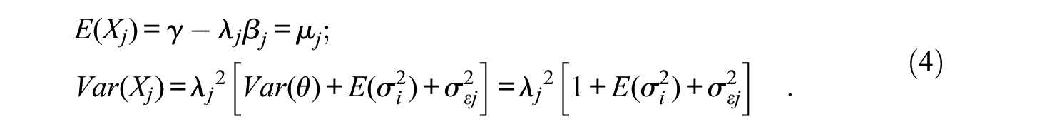
where $E({\sigma }_i^2)$ is the expected value of ${\sigma }_i^2$ in the population (i.e., the average of the PDDs). The covariance between X_j and X_k is

$$\mathrm{Cov}(X_j,X_k)={\lambda }_j{\lambda }_k\mathrm{Var}(\theta )={\lambda }_j{\lambda }_k.$$

(5)

We turn now to the factor analysis (FA) parameterization of the DTCRM. By making the transformation (Ferrando, 2009):

$${\beta }_j=\frac{\gamma -{\mu }_j}{{\lambda }_j},$$

(6)

the expectation in Equation (3) can be written as

$$E(X_{\mathrm{ij}}|{\theta }_i,{{\sigma }^2}_i)={\mu }_j+{\lambda }_j{\theta }_i.$$

(7)

which only depends on θ and is the structural equation of Spearman’s congeneric item score model (Mellenbergh, 1994). By further defining a j residual term as

$$u_j^2={{\lambda }_j}^2[E({\sigma }_i^2)+{\sigma }_{\epsilon j}^2].$$

(8)

The covariance structure implied by the DTCRM can be written as

$$\mathbf{C}=\mathbf{\lambda }\mathbf{\lambda }\prime +{\mathbf{U}}^2$$

(9)

where λ is the column vector containing the λ_j scaling weights, and U² is a diagonal matrix whose nonzero elements are the residuals in Equation (8). So, with the proposed transformations, the covariance structure for the DTCRM is then equivalent to that of the congeneric model.

The correlational structure corresponding to Equation (9) is

$$\mathbf{R}=\mathbf{\alpha }\mathbf{\alpha }\prime +{\mathbf{D}}^2,$$

(10)

where R is the interitem correlation matrix, the elements of α are the standardized loadings

$${\alpha }_j=\frac{{\lambda }_j}{\sqrt{\mathrm{Var}(X_j)}}=\frac{1}{\sqrt{1+E({\sigma }_i^2)+{\sigma }_{\epsilon j}^2}},$$

(11)

and the nonzero elements of the diagonal matrix D² are 1 −α _j ². It then follows from Equation (11) that

$$\frac{1-{{\alpha }^2}_j}{{{\alpha }^2}_j}=E({\sigma }_i^2)+{\sigma }_{\epsilon j}^2.$$

(12)

In the DTCRM formulation so far, X_j is bounded while θ is thought of as unbounded. So, the model cannot be strictly correct, since some values of θ would lead to expected values of X_j outside the boundaries of the item format. Rather, under this formulation, the item–trait regressions are expected to be nonlinear and heteroscedastic, with asymmetric conditional distributions and reduced variances toward the end of the scale. Therefore, the DTCRM must be viewed as an approximation (Mellenbergh, 1994). This approximation, however, is expected to work well when items are not too extreme and their loading values in Equation (11) are only moderate, which means that, in general, the item–trait regressions do not substantially depart from linearity, or, in other words, that they are well approximated by a straight line in the range of values that contains most of the respondents (Ferrando, 2002). Personality and attitude items generally fulfill the conditions above (Ferrando, 2002; Hofstee et al., 1998). So, the linear approximation is expected to work reasonably well with this type of item. On the other hand, in scenarios in which the items are both extreme and highly discriminating, a transformation of X_j may also make the transformed responses unbounded. This point is further discussed below.

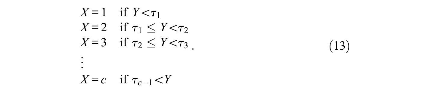
We turn now to the ordered-categorical-response case. Ferrando (2019) explicitly distinguished between a submodel for binary responses (DTBRM) and a submodel for graded responses (DTGRM). However, the DTBRM can be obtained as a particular case of the DTGRM simply by substituting the usual 0 to 1 scoring for the integer 1 to 2 scoring. So, we shall provide here a unified treatment, and revise only the DTGRM, which is based on the underlying-variables-approach (UVA, e.g., Edwards & Thurstone, 1952; Muthén, 1984). Let X_j be the observed item response, scored as 1, 2, . . ., c. The first part of the UVA assumes that there is an underlying, normally distributed latent variable Y_j that generates the observed item categorical score according to a step function governed by c − 1 thresholds (τ):

$$\begin{array}{cc}X=1\hfill & \mathrm{if}Y<{\tau }_1\hfill \\ \multicolumn{1}{c}{X=2}& \mathrm{if}{\tau }_1\le Y<{\tau }_2\hfill \\ \multicolumn{1}{c}{X=3}& \mathrm{if}{\tau }_2\le Y<{\tau }_3\hfill \\ \multicolumn{1}{c}{⋮}& \hfill \\ \multicolumn{1}{c}{X=c}& \mathrm{if}{\tau }_{c-1}<Y\hfill \end{array}.$$

(13)

In the present proposal, the second part of the UVA assumes that the structural model in Equations (1) and (2) holds for the underlying response variable Y_j

$$Y_{\mathrm{ij}}={\alpha }_j(T_i-b_j).$$

(14)

Compared with Equation (1) the midpoint intercept term γ is now zero, and the scale parameter λ_j is directly a standardized loading α_j (as in Equation 11). This is because the origin and scale for the latent Y_j are now undetermined, and this indeterminacy is (partly) solved by assuming that the scale midpoint is zero and the variance of the marginal distribution of Y_j is 1. With these restrictions, the marginal mean and variance of Y_j, are given by

$$\begin{array}{c}E(Y_j)=-{\alpha }_j{\beta }_j={\mu }_j;\hfill \\ \mathrm{Var}(Y_j)=1={{\alpha }_j}^2[1+E({\sigma }_i^2)+{\sigma }_{\epsilon j}^2].\hfill \end{array}$$

(15)

And the correlational structure and derived results for the Y_js are the same as in Equations (10) to (12).

In contrast to the DTCRM, the DTGRM explicitly treats the observed item scores as discrete and bounded, which is what they really are, so it is theoretically more plausible. Under this treatment, the observed item-trait regressions are nonlinear and heteroscedastic, the conditional distributions are asymmetric, and the variances are reduced toward the end of the scale. Whether this greater appropriateness translates into practical advantages with respect to the simpler, approximate DTCRM for the case of personality and attitude items is still not clear, however.

The Multidimensional Proposal: M-DTCRM and M-DTGRM

An extended formulation for the DTCRM in m (possibly correlated) dimensions can be obtained by assuming that, for each dimension k, item j has an element of location, denoted by β_jk, which is related to the position it occupies along the corresponding θ_k axis (this rationale is further discussed). The proposed structural equation of the M-DTCRM is

$$X_{\mathrm{ij}}=\gamma +{\lambda }_{j1}(T_{i1}-b_{j1})+\cdots +{\lambda }_{\mathrm{jm}}(T_{\mathrm{im}}-b_{\mathrm{jm}}),$$

(16)

where, for each individual i and each item j, the momentary trait values and the momentary item locations on each trait continuum are now vectors, and their elements are given by

$$T_{\mathrm{ik}}={\theta }_{\mathrm{ik}}+{\omega }_{\mathrm{ik}};b_{\mathrm{jk}}={\beta }_{\mathrm{jk}}+{\epsilon }_{\mathrm{jk}}.$$

(17)

The T_ik distributions over items are assumed to be normal with means θ_ik and common variance ${\sigma }_i^2$ . The distributions of b_j over respondents are assumed to be normal, with means β_jk, and variances ${\sigma }_{\epsilon j}^2$ . Finally, the item residuals of different dimensions are assumed to be independent, the person residuals of different dimensions are also assumed to be independent, and the item and person residuals are assumed to be independent from each other. So, apart from the full independence among residual terms, the model which is proposed assumes that (a) the variance over respondents around each β_jk, is the same ( ${\sigma }_{\epsilon j}^2$ ; it only depends on the item) and (b) the amount of person fluctuation ${\sigma }_i^2$ still remains constant over the different items of the questionnaire, even when these items measure different factors. Assumption (a) seems reasonable if the amount of IDD is viewed as a general characteristic of the item, and the plausibility of (b) is discussed below. From a practical point of view, all these new restrictions make model estimation feasible and allow stable estimates to be obtained. They also show that the conditional distribution of X_j for fixed θ_i and ${\sigma }_i^2$ is normal, and given by

$$\begin{array}{c}E(X_{\mathrm{ij}}|{\mathbf{\theta }}_{\mathbf{i}},{\sigma }_i^2)=\gamma +{\lambda }_{j1}({\theta }_{i1}-{\beta }_{j1})+\cdots +{\lambda }_{\mathrm{jm}}({\theta }_{\mathrm{im}}-{\beta }_{\mathrm{jm}});\hfill \\ \mathrm{Var}(X_{\mathrm{ij}}|{\mathbf{\theta }}_{\mathbf{i}},{\sigma }_i^2)=\left(\sum _k^m{{\lambda }_{\mathrm{jk}}}^2\right)({\sigma }_i^2+{\sigma }_{\epsilon j}^2).\hfill \end{array}$$

(18)

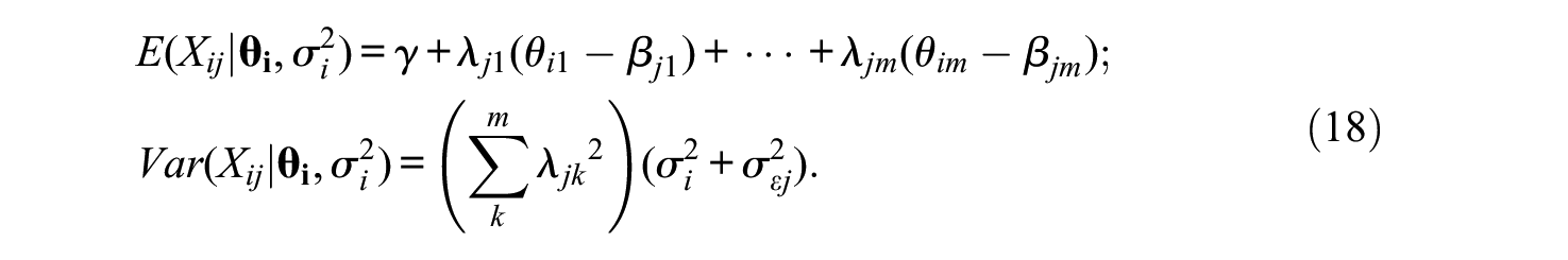
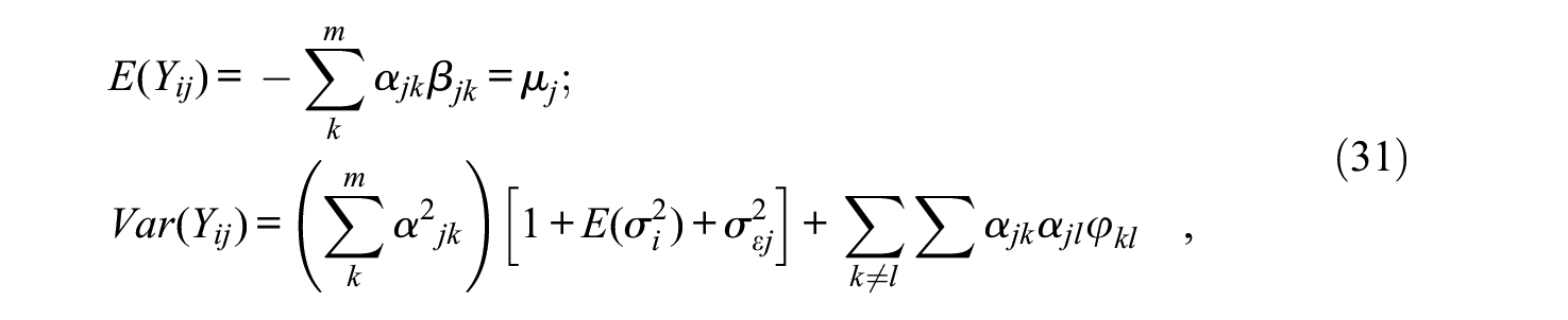
And, by assuming again that the marginal means and variances of the θ_ks are 0 and 1, respectively, the marginal mean and variance of X_j over the entire population of respondents are

$$\begin{array}{c}E(X_{\mathrm{ij}})=\gamma -\sum _k^m{\lambda }_{\mathrm{jk}}{\beta }_{\mathrm{jk}}={\mu }_j;\hfill \\ \mathrm{Var}(X_{\mathrm{ij}})=\left(\sum _k^m{{\lambda }^2}_{\mathrm{jk}}\right)[1+E({\sigma }_i^2)+{\sigma }_{\epsilon j}^2]+\sum _{k\ne l}\sum {\lambda }_{\mathrm{jk}}{\lambda }_{\mathrm{jl}}{\phi }_{\mathrm{kl}},\hfill \end{array}$$

(19)

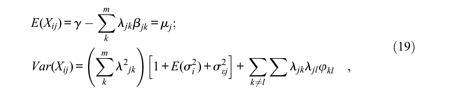
where φ_kl is the correlation between θ_k and θ_l (i.e., the interfactor correlation).

By using the definition,

$${\beta }_{\mathrm{jk}}=\frac{{\lambda }_{\mathrm{jk}}(\gamma -{\mu }_j)}{\sum _{k=1}^m{{\lambda }^2}_{\mathrm{jk}}}.$$

(20)

the expectation in Equation (18) can be written in standard FA form as

$$E(X_{\mathrm{ij}}|{\mathbf{\theta }}_{\mathbf{i}},{\sigma }_i^2)={\mu }_j+{\lambda }_{j1}{\theta }_{i1}+\cdots +{\lambda }_{\mathrm{jm}}{\theta }_{\mathrm{im}}.$$

(21)

And, by further defining a j residual term as

$$u_j^2=\left(\sum _k^m{{\lambda }^2}_{\mathrm{jk}}\right)[E({\sigma }_i^2)+{\sigma }_{\epsilon j}^2].$$

(22)

the covariance structure implied by the M-DTCRM can be written as

$$\mathbf{C}=\mathbf{\Lambda }\mathbf{\Phi }\mathbf{\Lambda }\prime +{\mathbf{U}}^2,$$

(23)

where Λ is the matrix containing the λ_jk scaling weights, Φ is the interfactor correlation matrix, and U² is a diagonal matrix whose nonzero elements are the residuals in Equation (22). The covariance structure (Equation 23) is indeed that of the standard correlated-factors FA model.

We shall now discuss the rationale for the choice of Equation (16) as the multidimensional extension of the DTCRM. Reckase (2009, chap 5) proposed a multidimensional difficulty (location) index, which, Ferrando (2009) adapted to the linear FA case. For the sake of simplicity we shall focus on the bidimensional case. Consider first the expectation in Equation (21) as a function defined on the (θ₁, θ₂) plane. The graph of this function is the item response surface of the bidimensional DTCRM and is a plane. The direction in which the slope of this plane is maximal can be determined, but, once a particular direction has been determined, the slope along it remains constant. Now, define the multidimensional location as the signed distance from the origin on the (θ₁, θ₂) plane to the point at which the expected item score is γ (the response scale midpoint) in the direction of the maximum slope of the item response surface (plane). This multidimensional location index, denoted by β_j, is given, in the general multidimensional case, by (see Ferrando, 2009)

$${\beta }_j=\frac{\gamma -{\mu }_j}{\sqrt{\sum _k^m{{\lambda }^2}_{\mathrm{jk}}}}.$$

(24)

It can be seen as a vector whose norm is intended to reflect the overall “difficulty” or extremeness of the item. The direction cosines that define the position of this vector (i.e., the direction of maximum slope) are given in the general case of m dimensions by (Ferrando, 2009)

$$\cos {\varphi }_{\mathrm{jk}}=\frac{{\lambda }_{\mathrm{jk}}}{\sqrt{\sum _k^m{{\lambda }^2}_{\mathrm{jk}}}}.$$

(25)

If we define the location element β_jk, in FA terms as in Equation (20), it then follows that

$$\begin{array}{c}{\beta }_{\mathrm{jk}}=\cos {\varphi }_{\mathrm{jk}}{\beta }_j\hfill \\ {{\beta }^2}_j=\sum _k^m{{\beta }^2}_{\mathrm{jk}}.\hfill \end{array}$$

(26)

So, each location element β_jk, is the orthogonal projection of the multidimensional location vector β_j on the θ_k axis. Overall then the rationale is to consider (a) a vector β_j that reflects the general “difficulty” or extremeness of the item and (b) the orthogonal projections of this vector on each θ_k axis as vectors that reflect the “difficulty” or extremeness of this item along this particular dimension. Note also that the element β_jk, can be interpreted as the contribution of the location element to the multidimensional location, and that this contribution will increase as the multidimensional location β_j vector gets closer to the corresponding θ_k axis.

The correlational structure corresponding to Equation (23) is

$$\mathbf{R}=\mathbf{A}\mathbf{\Phi }\mathbf{A}\prime +{\mathbf{D}}^2,$$

(27)

where the elements of A are the standardized loadings:

$${\alpha }_{\mathrm{jk}}=\frac{{\lambda }_{\mathrm{jk}}}{\sqrt{\mathrm{Var}(X_j)}}.$$

(28)

Finally, the multidimensional extension of Equation (12) is

$$\frac{1-{\mathbf{\alpha }\prime }_j\mathbf{\Phi }{\mathbf{\alpha }}_j}{{\mathbf{\alpha }\prime }_j{\mathbf{\alpha }}_j}=E({\sigma }_i^2)+{\sigma }_{\epsilon j}^2.$$

(29)

where ${\mathbf{\alpha }\prime }_j$ is the j row vector of A. As discussed below, the expression on the left-hand side of Equation (29) is a direct measure of IDD. As a simple and familiar auxiliary measure of overall item discriminating power, which has values between 0 and 1, the commonality estimate: ${\mathbf{\alpha }\prime }_j\mathbf{\Phi }{\mathbf{\alpha }}_j$ can also be used.

We turn now to the M-DTGRM, which will again be derived by using the UVA. The first part of the approach is the same as in Equation (13), because the relation between the observed and the latent response does not depend on the number of dimensions. As for the second part, we consider the modified multidimensional structure (Equation 16):

$$Y_{\mathrm{ij}}={\alpha }_{j1}(T_i\dots T_{\mathrm{im}}-b_{j1})+\cdots +{\alpha }_{\mathrm{jm}}(T_i\dots T_{\mathrm{im}}-b_{\mathrm{jm}}).$$

(30)

which has the same assumptions as detailed following Equations (16) to (18), and the additional restrictions that (a) the midpoint intercept term γ is zero, and (b) the scale parameters are directly standardized factor loadings α_jk. The marginal mean and variance of Y_j are

$$\begin{array}{c}E(Y_{\mathrm{ij}})=-\sum _k^m{\alpha }_{\mathrm{jk}}{\beta }_{\mathrm{jk}}={\mu }_j;\hfill \\ \mathrm{Var}(Y_{\mathrm{ij}})=\left(\sum _k^m{{\alpha }^2}_{\mathrm{jk}}\right)[1+E({\sigma }_i^2)+{\sigma }_{\epsilon j}^2]+\sum _{k\ne l}\sum {\alpha }_{\mathrm{jk}}{\alpha }_{\mathrm{jl}}{\phi }_{\mathrm{kl}},\hfill \end{array}$$

(31)

The multidimensional location index and the location elements are now given by

$${\beta }_j=\frac{-{\mu }_j}{\sqrt{\sum _k^m{{\alpha }^2}_{\mathrm{jk}}}}.$$

(32)

and,

$${\beta }_{\mathrm{jk}}=\frac{{\alpha }_{\mathrm{jk}}(-{\mu }_j)}{\sum _{k=1}^m{{\alpha }^2}_{\mathrm{jk}}}.$$

(33)

However, unlike in the M-DTCRM case, they cannot be obtained directly from the marginal means in Equation (19) because the latent responses Y_j cannot be observed. The identification conditions for estimating Equations (32) and (33) are discussed below. As for the correlational structure, it is the same as in the continuous case in Equation (27), and the result for identifying the sources of error is the same as in Equation (29).

Finally, we shall discuss the IRT modeling (conditional probabilities as they are used in the Supplemental Appendix; available online) of the M-DTGRM. The probability of scoring in the v category (i.e., X_j = ν) on item j for fixed θ _i and ${\sigma }_i^2$ is

$$\begin{array}{c}P(X_{\mathrm{ij}}=v|{\mathbf{\theta }}_i,{\sigma }_i^2)=\Phi \left(\frac{\mathbf{\alpha }\prime {\mathbf{\theta }}_i-(\mathbf{\alpha }\prime \mathbf{\beta }+{\tau }_{\mathrm{jv}-1})}{\sqrt{\mathbf{\alpha }\prime \mathbf{\alpha }}\sqrt{{\sigma }_i^2+{\sigma }_{\epsilon j}^2}}\right)-\Phi \left(\frac{\mathbf{\alpha }\prime {\mathbf{\theta }}_i-(\mathbf{\alpha }\prime \mathbf{\beta }+{\tau }_{\mathrm{jv}})}{\sqrt{\mathbf{\alpha }\prime \mathbf{\alpha }}\sqrt{{\sigma }_i^2+{\sigma }_{\epsilon j}^2}}\right)\hfill \\ =\Phi ({\mathbf{\xi }\prime }_{\mathrm{ij}}{\mathbf{\theta }}_i-{\delta }_{\mathrm{ijv}-1})-\Phi ({\mathbf{\xi }\prime }_{\mathrm{ij}}{\mathbf{\theta }}_i-{\delta }_{\mathrm{ijv}}).\hfill \end{array}$$

(34)

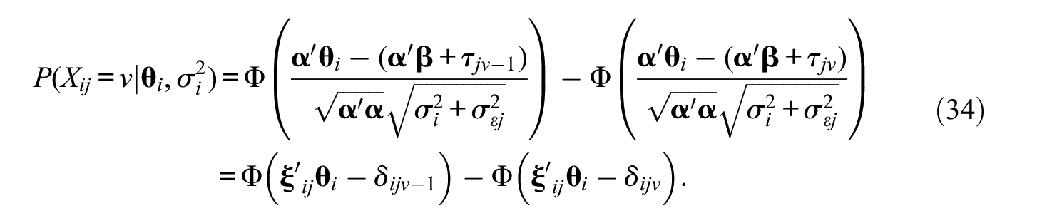
where Φ is the cumulative distribution function of the standard normal distribution. Note that the elements of the reparameterized discrimination vector ξ _ij (and also the reparameterized scalar location δ) depend on both item and person. Now, if the PDDs are equal for all the respondents (i.e., ${\sigma }_i^2$ = σ²) while the IDDs are allowed to vary over items, the discrimination vector will reduce to ξ _j , and the last expression in Equation (34) for the conditional probability will be that of the standard multidimensional normal-ogive graded response model (e.g., Reckase, 2009). The role of the PDD and the IDD in Equation (34) is the same as in the unidimensional case (see Ferrando, 2019). The θ _i vector determines the response category that has the greatest probability of being endorsed by i. As the PDD and the IDD approach zero, the probability of endorsing this category increases, whereas the probability of endorsing the remaining categories decreases. So, the response certainty increases (see, e.g., Tutz & Schauberger, 2020) and the response process becomes more and more deterministic.

Fitting the M-DTMs

The two-stage approach (calibration and scoring) proposed for the unidimensional models (Ferrando, 2019) is also proposed here so only relevant points related to the multidimensional expansion will be discussed below.

Item Calibration

In the most general scenario, a canonical unrestricted FA solution in m specified dimensions is fitted to the appropriate interitem correlation matrix: product–moment (M-DTCRM), or polychoric (M-DTGRM). The fit of the chosen model at the structural (correlational) level is then assessed, and finally the canonical solution is rotated to an interpretable solution with, generally, correlated factors. We note also that more restricted solutions, such as independent-cluster (confirmatory) or target rotations can also be fitted to the correlation matrix. In both cases (unrestricted or restricted), the estimates obtained by fitting the multiple FA solution are the standardized loadings α (Equations 28 and 30), the interfactor correlation matrix Φ (Equation 27) and the standardized residual variances. Now, for both the M-DTCRM and the M-DTGRM, Equation (29) shows a well-known result (e.g., Cronbach & Warrington, 1952; Torgerson, 1958): that the interitem correlation matrix does not contain sufficient information to separately identify the average PDD and IDDs. So, as in the unidimensional proposals, we chose the item with the smallest IDD as a marker for identifying the average PDD. In more detail, we chose as the marker the item for which the left-hand side of Equation (29) attains its minimal value, and we assumed that its IDD is zero. Then, relative to this scaling, the average PDD is estimated as

$${\left[\frac{1-{\mathbf{\alpha }}_{\prime }^j\mathbf{\Phi }{\mathbf{\alpha }}_j}{{\mathbf{\alpha }}_{\prime }^j{\mathbf{\alpha }}_j}\right]}_{(\min )}=\widehat{E}({\sigma }_i^2).$$

(35)

The results so far are common to both the M-DTCRM and the M-DTGRM.

The “marker” identification constraint used to obtain estimate Equation (35) is, in our view, unavoidable and very simple, but theoretically unsatisfactory, because it assumes that the best item in the bank is a “perfect” item with zero IDD, which is clearly unrealistic. So, the result of Equation (35) is best viewed as an upper bound for the average PDD rather than as a proper estimate. Perhaps better estimates could be obtained in scenarios in which more information is available (repeated measurements, multiple groups analyses, or already calibrated item banks). This is a point that clearly warrants further research.

We turn now to the item location parameters. In the M-DTCRM, we first need the Λ matrix containing the λ_jk scaling weights. It is estimated by

$$\mathbf{\Lambda }={\mathbf{D}}_{\mathbf{X}}\mathbf{A},$$

(36)

where D_X is the diagonal matrix containing the items’ standard deviations. Next, the location elements β_jk, are estimated using Equation (20) together with the marginal item means according to Equation (19). Finally, the multidimensional location index β_j, is obtained by using Equation (24).

In the M-DTGRM, the marginal means of the latent response variables are unknown, but assumed to be different among them (Equation 31). So, constraints on the thresholds should be applied to identify these means, and we propose here to use those by Lubbe and Schuster (2017): to fix the middle threshold (even number of categories) or the sum of the two central thresholds (odd number of categories) to zero. With these constraints, the original thresholds are completely determined by the probabilities of the categorized outcomes (Equation 13) and, within each item, the transformed thresholds differ from the original ones by a constant term which is the latent mean of Y_j (i.e., µ_j). Once this estimate has been obtained, both β_j and the β_jks can be further estimated by Equations (32) and (33). We should point out that, with the proposed constraints, the estimates of β_j, and β_jk, obtained from the M-DTCRM and the M-DTGRM were almost identical in all the previous checks we made.

Individual Scoring and Score-Based Measures of Accuracy and Appropriateness

The approach proposed for estimating the individual parameters in the M-DTCRM and the M-DTGRM is a straightforward extension of the one proposed for the original unidimensional models (Ferrando, 2019). So it will only be summarized here and more details are provided in the Supplemental Appendix (available online). The estimates are Bayes expected a posteriori (EAP, Bock & Mislevy, 1982); the priors for the θs are standard normal, the prior for the PDDs is the scaled inverse χ² distribution (Novick & Jackson, 1974), and both types of priors are approximated by rectangular quadrature.

For each individual i, the outcome of the scoring process consists of (a) m point estimates of the central trait levels of this individual on each factor ( ${\hat{\theta }}_{\mathrm{ik}}$ ); (b) the PDD point estimate ( ${\hat{\sigma }}_{\mathrm{ik}}^2$ ) assumed to be constant over dimensions; and (c) the m+ 1 posterior standard deviations (PSDs) corresponding to each point estimate, which would serve as standard errors (e.g., Bock & Mislevy, 1982). By extending Bock and Mislevy’s (1982) proposal, PSD-based conditional reliability estimates can further be obtained as

$$\begin{array}{c}\rho ({\hat{\theta }}_{\mathrm{ik}})=1-\frac{\mathrm{PSD}{({\hat{\theta }}_{\mathrm{ik}})}^2}{\mathrm{Var}({\theta }_k)}=1-\mathrm{PSD}({\hat{\theta }}_{\mathrm{ik}}{)}^2\hfill \\ \rho ({{\hat{\sigma }}^2}_i)=1-\frac{\mathrm{PSD}{({{\hat{\sigma }}^2}_i)}^2}{\mathrm{Var}({\sigma }^2)},\hfill \end{array}$$

(37)

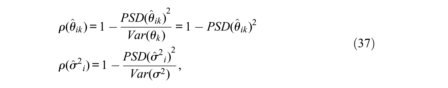
where Var(θ_k) refers to the population variance of the k trait and Var(σ²) refers to the population variance of the PDDs. As stated above, the population trait variances are all fixed at 1. As for Var(σ²) we use the empirical estimate obtained from the ${{\hat{\sigma }}_{\mathrm{ik}}}^2$ point estimates (Brown & Croudace, 2015).

As overall measures that assess the precision of the estimates in the population of respondents, empirical marginal reliability estimates can be obtained by averaging the squared PSDs in the sample of N individuals (Brown & Croudace, 2015):

$$\begin{array}{c}\overline{\rho }({\hat{\theta }}_k)=1-\frac{\sum _i^N{[\mathrm{PSD}({\hat{\theta }}_{\mathrm{ik}})]}^2}{\mathrm{NVar}({\theta }_k)}=1-\frac{\sum _i^N{[\mathrm{PSD}({\hat{\theta }}_{\mathrm{ik}})]}^2}{N}\hfill \\ \overline{\rho }({\hat{\sigma }}^2)=1-\frac{\sum _i^N{[\mathrm{PSD}({{\hat{\sigma }}^2}_i)]}^2}{\mathrm{NVar}({\sigma }^2)}\hfill \end{array}.$$

(38)

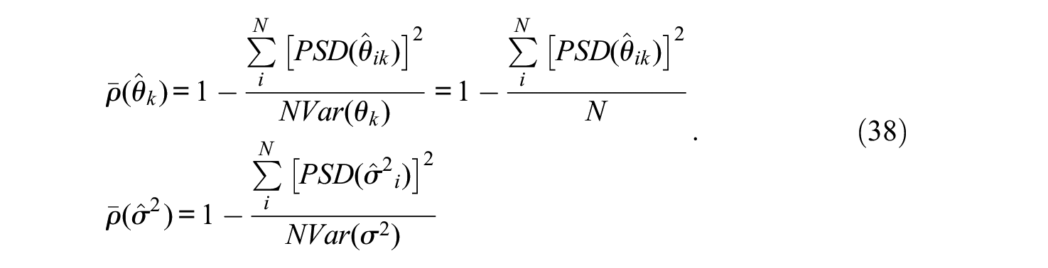
As it should be, for both θ_k and σ² the conditional and marginal reliability estimates in Equations (37) and (38) are unitless numbers between 0 and 1 that do not depend on the particular choices of Var(θ_k) and Var(σ²).

We turn now to the assessment of model appropriateness. The multiple FA model based on product–moment interitem correlations, and the corresponding UVA-based model based on polychoric correlations can be viewed as restricted versions of the M-DTCRM and the M-DTGRM, respectively, and are obtained from the latter by restricting the PDDs to be the same for all respondents. Furthermore, at the structural level each “normative” FA model (i.e., equal PDDs) and its corresponding DM are indistinguishable, as they give rise to the same correlational structure. So, the greater appropriateness of the more flexible but complex DM with regard to the more restricted normative model must be assessed from the individual estimates.

The common approach used in previous developments is based on a likelihood ratio (LR) statistic. For a single respondent i, let $L_i^0({\hat{\mathbf{\theta }}}_i,{\hat{\sigma }}^2)$ be the value of the likelihood function evaluated by using the vector of central trait estimates obtained under the restriction that all the PDDs have a constant value. Now, let $L_i^1({\hat{\mathbf{\theta }}}_i,{{\hat{\sigma }}_i}^2)$ be the corresponding value using both the person locations and the PDD estimate. The LR statistic and the transformed value also proposed here are

$${\Lambda }_i=\frac{L_i^0({\hat{\mathbf{\theta }}}_i,{\hat{\sigma }}^2)}{L_i^1({\hat{\mathbf{\theta }}}_i,{{\hat{\sigma }}_i}^2)};s_i=-2\ln ({\Lambda }_i).$$

(39)

Statistic Λ_i is a descriptive normed index with values in the range 0 to 1. Values close to 0 indicate that the dual TM provides a substantially better fit than the corresponding standard model. As for s_i, it is a χ²-type statistic, and the sum Q = Σs_i is also a χ²-type statistic referred (approximately) to a χ² distribution with N degrees of freedom (see Ferrando, 2013, 2019). We should stress that Q is only meant to be used as a useful approximate reference, not as a strict test of fit. In this respect, simulation results in the unidimensional case suggest that it is a conservative index, which is only to be expected, because (a) in an LR test the likelihoods must be evaluated at their ML estimates whereas here they are evaluated at their EAP estimates, and (b) these EAP estimates are regressed toward the mean, which brings them closer to the constant PDD restriction than the more “spread out” ML estimates would be.

Substantive and Practical Considerations

Dual Thurstonian models are more flexible than their normative counterparts, but this flexibility has a price in terms of complexity and proneness to providing unstable or implausible estimates. In the multidimensional case dealt with here, we have addressed this issue by imposing additional restrictions that keep the models relatively simple and allow plausible person estimates to be obtained for all the respondents in realistic conditions.

The most important restriction we propose is that the amount of person fluctuation is the same over the different items, even when these items measure different dimensions. However, the amount of PDD might well be (at least partly) intrinsic to the trait being measured (Taylor, 1977). If so, the present proposal would be most plausible in the case of questionnaires designed to measure related dimensions that, to a greater or lesser extent, are influenced by a more general dimension (such as a second-order factor). At the other extreme, the restriction would possibly be unrealistic for instruments that aim to measure broad and unrelated personality traits. In this case, the person estimate ${\sigma }_i^2$ would probably reflect the average fluctuation of this individual across the different traits.

A second potential practical concern of the proposal lies in identifying the average PDD at the calibration stage based on the most discriminating item (Equation 35). The presence of one or more items with unusually high communality estimates would result in a near-zero estimate for the average PDD, which, in turn, would make valid assessment of individual differences in PDD difficult. In FA terms, this problem is that of a quasi-Heywood case (see Lorenzo-Seva & Ferrando, 2020), and is expected to be worse here than in the unidimensional case, especially for the M-DTGRM. The presence of redundant items that are nearly linear composites of the remaining test items, and particularly doublets and triplets (McDonald, 1985), overfactoring, poorly defined factors (McDonald, 1985), and excessive sampling variability are, among, other things, potential causes of this phenomenon (see Lorenzo-Seva & Ferrando, 2020, for a detailed discussion). Our recommendation is to (a) “clean” the data set and remove the offending items before applying the DM and (b) avoid overfactoring when fitting the model.

Finally, we shall move on to discuss the potential practical advantages of using the models proposed here. As discussed in greater depth in Ferrando (2019) there are three main ones. First, they provide additional information about the response consistency of the individual when answering the test. Second, they allow a meaningful assessment of the differential accuracy of the central trait point estimates as a function of the amount of PDD. Finally, the PDD estimates might have a moderating role in external validity assessment: Individuals with small PDDs are expected to be more predictable (see Ferrando, 2019). However, the moderating effects of the PDD in practice are expected to be modest at best (Ferrando, 2013, 2019).

The second advantage above (differential accuracy) is illustrated in Figure 1 using one of the data sets of the simulation study. It is a three-factor solution, and the ordinate axis shows the conditional reliability of the factor score estimates (Equation 37) averaged across the three factors, as a function of the amount of PDD.

Figure 1.

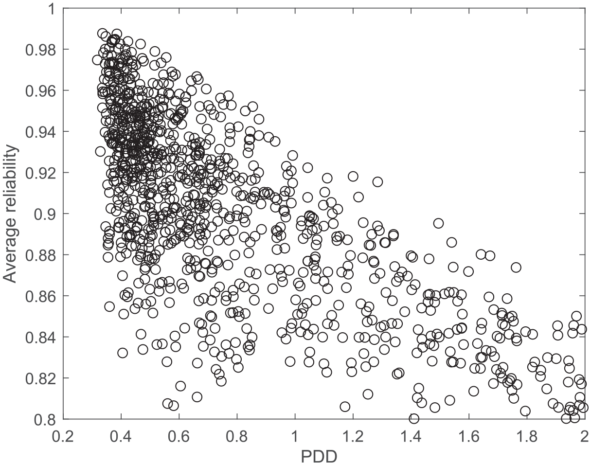
Average conditional reliability over factors as a function of person discriminal dispersion.

Two main results are apparent from the graph. First, the accuracy of the individual trait estimates decreases with the amount of person fluctuation, as expected. Second, the variability of the conditional reliabilities also depends on the amount of PDD, the scatter approaching the so-called “twisted-pear” contour (Fisher, 1959). When the amount of person fluctuation is low, the accuracy of the trait estimates mainly depends on the trait level, so accuracy can vary considerably. On the other hand, however, high PDD values mean that the trait estimates cannot be very accurate no matter what the trait levels are. The expected differential accuracy of the trait estimates as a function of the amount of PDD is empirically assessed in the illustrative example.

Simulation Studies

For both the M-DTCRM and the M-DGRM, two initial simulation studies were carried out to (a) check the correctness of the results and expectations derived from the proposal and (b) assess the functioning of the estimation procedures proposed. The complete studies as well as the tables of results are presented in the Supplemental Appendix (available online), and only a summary is given here.

For each of the two models, the study had two parts. The first part assessed whether appropriate calibration results could be attained. The second part assessed the expected conditions under which accurate individual estimates could be obtained. So, the first part of the study was essentially a model check and aimed to assess whether data generated from a multidimensional dual model did in fact behave like a multiple FA model at the correlational level. More in detail, what was assessed was whether the items could be well calibrated by fitting a FA solution to the appropriate (Pearson or polychoric) interitem correlation matrix in which (a) the correct number of factors was specified and (b) the direct solution was rotated using a semispecified oblique target rotation with a target matrix that was congruent with the “true” pattern. The calibration results were quite clear: For both models, and in all conditions, when the number of factors and the expected target matrix were well specified, the structural solution was well recovered and the model–data fit was good.

The main focus of the second part of the study was on whether the “true” individual parameters could be appropriately and accurately recovered. Results were also positive and agreed with expectations. In summary, for items of reasonable quality, accurate trait estimates are expected to be obtained from small instruments or item sets with two factors and seven items per factor. Reasonably accurate PDD estimates, however, require larger item sets, but can be obtained from moderately large instruments of about 25 items and two or three factors.

Implementation

The proposal so far is contained in an existing R package: InDisc (Ferrando & Navarro-González, 2020). Originally, this package was designed for fitting the unidimensional IRT dual models described in Ferrando (2019). Several modifications have been made so that the multidimensional models (up to four dimensions) can be assessed. The usage is the same as that described in the original article: It consists of a main function (InDisc), which calls all the subfunctions required for (a) item calibration in the first stage and (b) item scoring in the second stage (including measures of reliability and model appropriateness).

The new version of InDisc has been developed in R Version 4.0.2 and runs with R versions more recent than 3.5.0. The number of variables and respondents the program can handle is not limited but can heavily impact computing time.

Illustrative Example

A data set containing the responses of 384 undergraduates to the Statistical Anxiety Scale (SAS; Vigil-Colet et al., 2008) was reanalyzed with the M-DTCRM and the M-DTGRM. It had been previously fitted with standard procedures (Ferrando & Lorenzo-Seva, 2019), and more details can be found there. As a summary, the SAS is a 24-item measure intended to assess the anxiety levels of students taking a statistics course. It was designed for assessing three related dimensions: Examination Anxiety (eight items), Asking for Help Anxiety (eight items), and Interpretation Anxiety (eight items). All of the items are positively worded and use a five-point Likert-type response format, ranging from no anxiety (1) to considerable anxiety (5).

Previous analyses not only obtained a clear solution in three highly related factors that matched the theoretical structure but also found that an essentially unidimensional solution was tenable. Additional assessment concluded not only that information and accuracy were greater when the tridimensional solution was used but also that the use of total raw (or factor) scores as if they were essentially unidimensional was acceptable. So, the dataset is “a priori” appropriate for the present proposal. On the one hand, the strong interfactor relations and essential unidimensionality suggest that the assumption of constant PDD over items is plausible. On the other, fitting the DTCRM or the DTGRM to short sets of five to eight items is practically unfeasible if accurate estimates of the person parameters (particularly the PDDs) are to be obtained.

Although both the M-DTCRM and the M-DTGRM were fitted to the data, we found that (a) the results provided by both models agree closely (as expected) but (b) the simpler M-DTCRM fitted the data slightly better and provided clearer results in this case. For this reason, only the M-DTCRM–based results are reported here.

Item Calibration

A canonical solution in three factors was fitted to the interitem product–moment correlation matrix by using robust unweighted least squares estimation as implemented in the FACTOR program (Lorenzo-Seva & Ferrando, 2013) and then obliquely rotating using Promin (Lorenzo-Seva, 1999). Goodness-of fit was assessed by using both the conventional approach and the equivalence testing approach by Yuan et al. (2016). The fit results were excellent, and are indeed the same as those reported in Ferrando and Lorenzo-Seva (2019), who used the same fitting procedure.

Table 1 shows the rotated pattern of standardized loadings (A) and the interfactor correlation matrix (Φ) together with the communality estimates ( ${\mathbf{\alpha }\prime }_{\mathbf{j}}\mathbf{\Phi }{\mathbf{\alpha }}_{\mathbf{j}}$ ), which, as discussed below (Equation 29), are measures of overall item discriminating power. As in the previous analyses, the rotated pattern agrees quite well with the prescribed “a priori” structure, with all the salient loadings (boldfaced) located in the corresponding factor, and with the three factors positively and substantially correlated with each other. Note that the item communalities tend to be rather high, which indicates not only high internal consistency but also possibly a certain amount of redundancy, as the item contents are quite similar. The most discriminating item is 17, which was chosen as a marker for obtaining the initial estimate of the average PDD. The initial estimate of the average PDD obtained using Equation (29) was $E({\sigma }_{i•}^2)=0.30$ The final empirical estimate based on the average of the individual estimates was $E({\sigma }_{i•}^2)=0.45$ .

Table 1.

Calibration Results. Illustrative Example.

(a) Rotated pattern of standardized loadings with the communality estimates
	F1	F2	F3	Communality estimates
I1	0.0156	0.6803	0.0200	0.4974
I2	–0.2636	–0.2636	0.8115	0.4197
I3	0.9521	–0.0312	–0.2236	0.6520
I4	–0.0811	0.7738	–0.0500	0.4720
I5	0.6025	–0.1295	0.2081	0.4378
I6	–0.0536	–0.1971	0.8281	0.4603
I7	0.9214	–0.0654	–0.0537	0.7131
I8	0.1609	0.1885	0.3628	0.4047
I9	–0.0163	0.8675	–0.1797	0.5543
I10	–0.1954	–0.1165	0.7516	0.3392
I11	0.0283	0.8156	–0.1747	0.5261
I12	0.9606	–0.0488	–0.1517	0.7056
I13	–0.2043	0.8214	–0.0636	0.4303
I14	0.1105	0.6572	–0.0516	0.4944
I15	–0.2577	0.9808	–0.1280	0.5605
I16	0.0526	0.1821	0.3024	0.2372
I17 a	0.9726	–0.1155	–0.0786	0.7225
I18	–0.0195	–0.0708	0.6331	0.3305
I19	0.1245	0.0671	0.4741	0.3761
I20	–0.2147	0.9139	–0.0862	0.5294
I21	0.7080	–0.1985	0.2835	0.6047
I22	–0.1210	–0.1261	0.9144	0.5871
I23	0.9714	–0.0577	–0.1908	0.6821
I24	0.7240	–0.1645	0.1750	0.5383
(b) Interfactor correlation matrix
	F1	F2	F3
F1	1	0.6997	0.6422
F2	0.6997	1	0.6889
F3	0.6422	0.6889	1

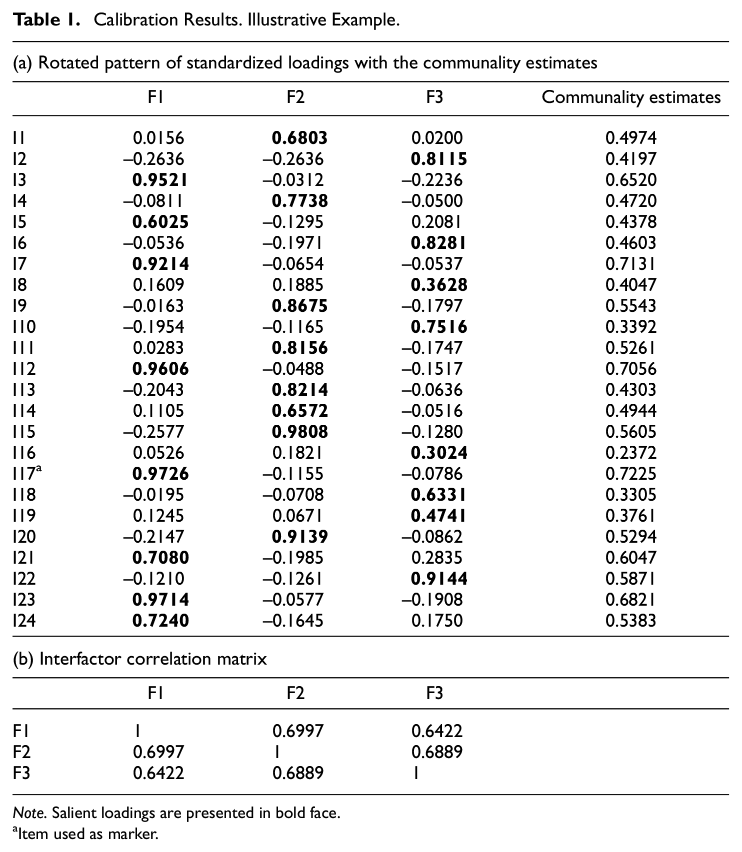
Note. Salient loadings are presented in bold face.

a

Item used as marker.

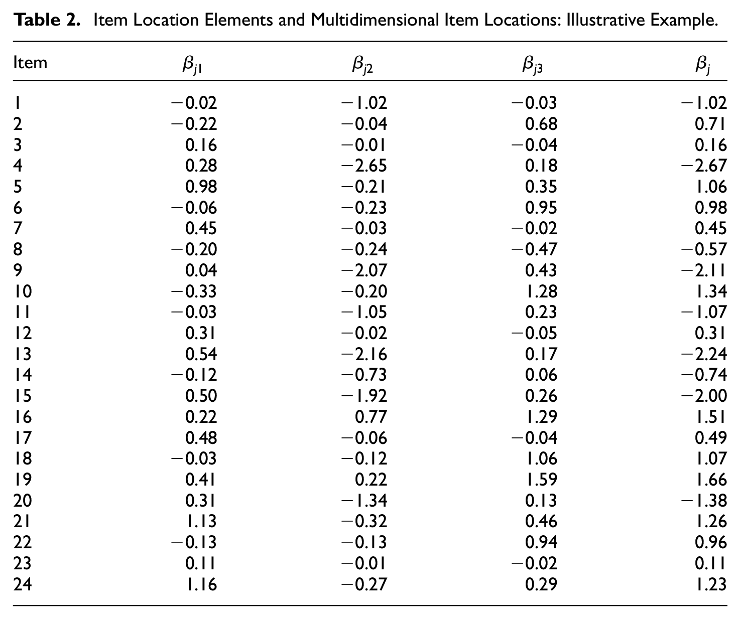
We turn now to the item location measures. For each item, Table 2 shows (a) the location elements along each factor (Equation 33) and (b) the multidimensional location in Equation (32). First, note that, overall, the items tend to be “easy” (i.e., very low levels of anxiety are required to agree with the item content). Second, the most extreme items (e.g., Item 4) tend to be aligned along the second factor, which is “Examination Anxiety.”

Table 2.

Item Location Elements and Multidimensional Item Locations: Illustrative Example.

Item	${\beta }_{j1}$	${\beta }_{j2}$	${\beta }_{j3}$	${\beta }_j$
1	−0.02	−1.02	−0.03	−1.02
2	−0.22	−0.04	0.68	0.71
3	0.16	−0.01	−0.04	0.16
4	0.28	−2.65	0.18	−2.67
5	0.98	−0.21	0.35	1.06
6	−0.06	−0.23	0.95	0.98
7	0.45	−0.03	−0.02	0.45
8	−0.20	−0.24	−0.47	−0.57
9	0.04	−2.07	0.43	−2.11
10	−0.33	−0.20	1.28	1.34
11	−0.03	−1.05	0.23	−1.07
12	0.31	−0.02	−0.05	0.31
13	0.54	−2.16	0.17	−2.24
14	−0.12	−0.73	0.06	−0.74
15	0.50	−1.92	0.26	−2.00
16	0.22	0.77	1.29	1.51
17	0.48	−0.06	−0.04	0.49
18	−0.03	−0.12	1.06	1.07
19	0.41	0.22	1.59	1.66
20	0.31	−1.34	0.13	−1.38
21	1.13	−0.32	0.46	1.26
22	−0.13	−0.13	0.94	0.96
23	0.11	−0.01	−0.02	0.11
24	1.16	−0.27	0.29	1.23

Individual Scoring and Score-Based Measures of Accuracy and Appropriateness

EAP score estimates for the three content dimensions and the PDDs, together with their corresponding PSDs, were obtained as described in the Supplemental Appendix (available online). The accuracy of the resulting estimates was assessed in two ways. First, the PSD-based marginal reliability estimates were obtained according to Equations (38). Second, empirical split-half reliability estimates were obtained by using the standard approach: The correlations between the estimated EAP scores based on equivalent halves were first obtained, and then they were stepped-out using the Spearman–Brown prophecy. The results are in Table 3.

Table 3.

PSD-Based and Split-Half–Based Marginal Reliability Estimates: Illustrative Example.

	θ 1	θ 2	θ 3	${\sigma }_i^2$
PSD-based	.93	.90	.85	.63
Split-half	.91	.91	.89	.60

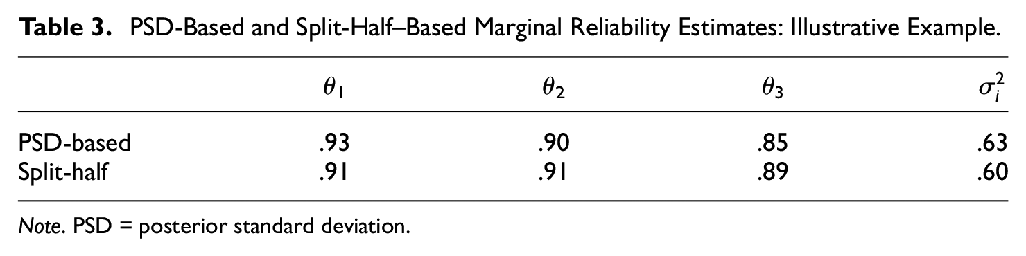
Note. PSD = posterior standard deviation.

Overall, there is good agreement between the outcomes produced by the two reliability approaches. Note that the marginal reliabilities of the content scores are quite high, but those of the PDD estimates are far lower. These results are generally in agreement with those of the simulation study in the situation most similar to this one (21 items/three factors, large item discriminations, and medium sample size; see Table 6 in the Supplemental Appendix).

We turn finally to the score-based measures of model appropriateness. The average of the LR Λ_i estimates was 0.29, and the Q = Σs_i value was 531.21 with 384 degrees of freedom as a reference (see Equation 39). Taken together, these results suggest that the M-DTCRM is more appropriate than the corresponding normative model. This potential appropriateness is assessed in the next section using additional evidence.

The Role of PDD in the Accuracy and Validity of Trait Scores: Extended Analyses

As discussed above, other things being equal, more accurate trait estimates should be obtained for individuals with low PDD (see Figure 1). To check this prediction with real data, we extended the split-half schema above in two ways. First, we used moderated multiple regression (e.g., Baron & Kenny, 1986) to see if the PDD estimates had a role in moderating the correlations between the content factor score estimates based on the two test halves. Second, two extreme subgroups (low-PDD and high-PDD) were formed using Cureton’s (1957) 27% rule, and the split-half correlations between the three factor score estimates were obtained. For the first procedure, significant results in the expected direction at the .05 level were obtained for the first two factors, in which R² increased from .60 to .64 (F1) and .60 to .62 (F2). As for the second, Table 4 shows the split-half correlations in each group, together with the corresponding 90% confidence intervals.

Table 4.

Split-Half Correlations Between the Trait Estimates in the Low-PDD and High-PDD Groups: Illustrative Example.

	θ 1	θ 2	θ 3
Low-PDD	.95 (.93, .96)	.90 (.86, .93)	.88 (.83, .91)
High-PDD	.57 (.42, .67)	.64 (.51, .73)	.70 (.59, .78)

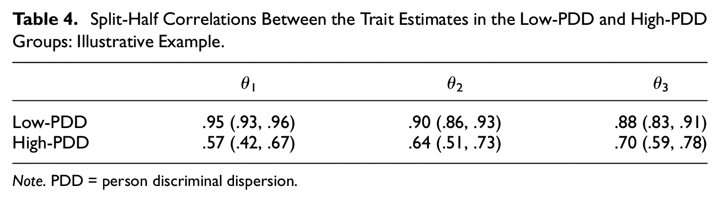
Note. PDD = person discriminal dispersion.

The results from both procedures are in agreement, and they are quite clear: As expected, the accuracy of the “content” factor estimates is greater for the individuals with low PDD.

Finally, we shall assess the role of PDD as a potential moderator of validity relations with external variables. For 238 respondents, the marks on a final statistical exam were available and were used as a criterion. We again used the extreme-groups approach based on the 27% rule (Low-PDD vs. High-PDD) and chose as a measure the multiple R between the criterion and the EAP score estimates on the three content factors. For the low-PDD group, R and the 90% confidence interval were .55 and (.38, .69). For the high-PDD group, they were .47 and (.23, .57). So, the results are in the expected directions, but the intervals overlap, and so differential validity cannot be considered to be significant.

Discussion

The starting point of this article is that DMs are a flexible and plausible way of modeling personality item scores, and that their use in applications shows promise both at the substantive and practical levels. If this is so, existing models clearly need to be extended to the multidimensional case for both substantive and practical reasons. Substantively, most personality questionnaires are multidimensional. At the practical level, minimally accurate person fluctuation estimates necessarily require a relatively large number of items, and this requirement makes it unfeasible to fit multidimensional measures on a scale-by-scale basis.

The multidimensional extension of the existing DMs has been developed on the basis of the concept of a general item location index that can be viewed as a vector. Projections of this vector on each factorial axis provide a location element along each dimension, which, in turn, allows the response mechanism considered in the unidimensional case to be extended to all the dimensions under study. The results obtained from this approach are plausible and can be considered as natural extensions of the previous unidimensional proposals.

Overall, the modeling proposal as well as the estimation and scoring procedures have been purposely kept as simple and robust as possible. Thus, a simple two-stage estimation approach (calibration and scoring) is proposed in which the calibration is generally based on unweighted least squares estimation, while the score estimates are obtained using Bayes EAP estimation. The most important simplification, however, is that the person fluctuation parameter (the PDD), which is the most important contribution of the DM at the individual level, is considered to be constant over test items. This restriction allows for a “borrowing strength” mechanism in which more stable estimates are obtained based on all the items, regardless of the particular factors on which they mainly load. The simulation results suggest that the restriction functions quite well as far as parameter recovery is concerned, and the illustrative example arrived at plausible results and behaved in accordance with the expectations derived from the simulation results. However, whether our simple proposal is plausible in practice requires further research.

If the usefulness of the proposal is supported by further evidence, many points can be worked on and improved. To start with, as discussed above, the M-DTCRM can be viewed as an approximation in the case of (necessarily) bounded item scores. Furthermore, in situations in which the item-factor regressions are expected to be markedly nonlinear, this approximation would probably be poor, and an alternative approach should be considered. The most workable approach may be to apply a logit transformation to the direct scores, use the UVA, and assume that the M-DTCRM, as is proposed here, holds for the transformed scores. The nonlinear relations between the factors and the original scores could then be obtained as in Ferrando (2002), and the result would be a continuous item response model with additional person parameters. Apart from this new development, more sophisticated procedures for estimating parameters and assessing model–data fit could be attempted, and recommendations and cutoff or reference values obtained from further intensive simulation could be proposed. For the moment, experience suggests that proposals such as the present one can be used in practice only if they are implemented in widely available (and preferably free) programs, and we note that this is the case here. The R package InDisc implements the procedures described in this article, and it is already fully available for the interested readers and practitioners from the CRAN website (https://cran.r-project.org/package=InDisc).

Supplemental Material

sj-pdf-1-epm-10.1177_0013164421998412 – Supplemental material for A Multidimensional Item Response Theory Model for Continuous and Graded Responses With Error in Persons and Items

Supplemental material, sj-pdf-1-epm-10.1177_0013164421998412 for A Multidimensional Item Response Theory Model for Continuous and Graded Responses With Error in Persons and Items by Pere J. Ferrando and David Navarro-González in Educational and Psychological Measurement