
Abstract
This study develops a theoretical model for the costs of an exam as a function of its duration. Two kind of costs are distinguished: (1) the costs of measurement errors and (2) the costs of the measurement. Both costs are expressed in time of the student. Based on a classical test theory model, enriched with assumptions on the context, the costs of the exam can be expressed as a function of various parameters, including the duration of the exam. It is shown that these costs can be minimized in time. Applied in a real example with reliability .80, the outcome is that the optimal exam time would be much shorter and would have reliability .675. The consequences of the model are investigated and discussed. One of the consequences is that optimal exam duration depends on the study load of the course, all other things being equal. It is argued that it is worthwhile to investigate empirically how much time students spend on preparing for resits. Six variants of the model are distinguished, which differ in their weights of the errors and in the way grades affect how much time students study for the resit.
Introduction
Exams at universities typically take between 0.5 and 5 hours, but what is the optimal duration? Recently, this was discussed by the faculty of the psychology department of the Radboud University, and several faculty members suggested that the courses with high study load require longer exams. The other side of this argument is that short exams, of say 1 hour, would suffice for small courses. Since I am Chairman of the Examination Board of the psychology program, my opinion on this matter was asked. My first thought on this was that a shorter exam will have less questions, and consequently a lower reliability, and that this might breach the common standards of reliability. For example, the Dutch Committee on Tests and Testing states that the reliability of a test being used for “important decisions at individual level” should be at least 0.80 (Evers et al., 2019, p. 34). However, the department is not bound by this regulation, and Ellis (2013) argued against such arbitrary reliability standards. Therefore, let us consider explicitly what the problems of a short test would be.
The main problem of a short test is that the inevitable measurement errors will be relatively large. Consequently, there will be more students who fail the exam while they should have passed, and more students who pass the exam while they should have failed. But to how many students does this happen? In order to make an informed decision, we want to quantify this. The next section will develop a simple classical test theory model for this.
The next question is what the costs of such incorrect decisions are. If the student fails, the student will retake the exam later, and for this the student needs additional study time. The present study will consider this time as the costs for the student. If the student passes undeservedly, it is harder to quantify the costs. In this case, there are usually no extra costs for the student, but there may be costs for the institution in terms of reputation damage if future employers or teachers note the lack of skills of some students who passed this exam. However, this kind of costs is much harder to quantify, and therefore it will be ignored in most of the article.
Having a long exam, on the other hand, has also costs, because all students of the course will have to spend time on this. Based on these ingredients, the optimum exam duration may be defined as the exam duration for which the total costs in the student population are minimal, where the total costs are computed as (1) the hours extra study time for students who failed incorrectly plus (2) the hours spent by all students on the examination. This article will demonstrate that this optimum is easily computed if the relevant statistics are known from a previous administration.
Obviously, there are in fact also other costs for the student, such as emotional stress. There will also be additional costs for the institution, such as the need of a bigger exam hall during the resit if more students fail. Furthermore, the costs of correcting the exam are ignored, which might be defensible for multiple choice exams that are automatically processed. Furthermore, one might argue that an item response theory model is needed instead of classical test theory. All these improvements will be ignored for the sake of simplicity of the model.
The next section describes how the present article is related to articles with similar objectives. The following sections will explicate the test score model and explain how the probability of an incorrect fail on the exam can be derived from it, and include the two costs in the model and define the objective function. After illustrating this model with a real exam in discrete time, it will be shown that with continuous time, the objective function is convex and has a unique minimum. The following section will investigate numerically how the minimum depends on the parameters. Several other versions of the model are discussed briefly.
Previous Optimization Approaches
This section will sketch how the method developed in the present article differs from earlier approaches. Several authors have studied how one can optimize generalizability coefficients, reliability coefficients, or validity coefficients, or how one can minimize decision error rates. In many cases this was studied in the context of a budget constraint (e.g., Allison et al., 1997; Ellis, 2013; Liu, 2003; Marcoulides, 1993, 1995, 1997; Marcoulides & Goldstein, 1990a, 1990b, 1992; Meyer et al., 2013; Sanders, 1992; Sanders et al., 1991) or fixed total testing time (e.g., Ebel, 1953; Hambleton, 1987; Horst, 1949, 1951). Alternatively, one may minimize the costs of measurement given constraints on the generalizability coefficient or error variance (e.g., Peng et al., 2012; Sanders et al., 1989), which is a similar problem. In these cases, the measurements have multiple facets (such as items and subjects) or multiple components (such as subtests), each associated with different costs or durations. The optimization achieves a balance of these facets or components. The present study, in contrast, does not assume a priori constraints on the budget, testing time, generalizability coefficient, error variance, or error rate. Instead, it specifies not only the costs of measurements but also the costs of decision errors—unlike the studies cited above. These two kinds of costs will be balanced via minimization of the expected loss.
Many of the articles cited above use the Spearman–Brown formula, and this will be used in the present study too. Several articles assume continuous parameters, because this permits the use of derivatives. The present study will do that too.
A different branch of psychometric optimization is the selection of items in Computerized Adaptive Testing (e.g., Wiberg, 2003), maximizing Cronbach’s alpha (Flebus, 1990; Thompson, 1990), or creating test forms (e.g., Raborn et al., 2020). In these studies there is a constraint on the test length or the error variance. The present study does not use such constraints. Furthermore, these studies assume that the test items have different psychometric parameters, which are being used in the optimization, while the present study assumes test items that are equivalent with respect to psychometric parameters and costs.
Assuming that errors cost something is naturally done in decision problems in economics or industry. In educational testing, such assumptions are usually avoided because there is no obvious, generally agreed-upon method to quantify the costs of errors in pass/fail decisions. But is it possible to create defensible quantifications of such costs? Examiners will anyhow make exams of a certain length. Thus, at a certain point the examiner stops increasing the test length and implicitly accepts the corresponding error rate. Therefore, every finite exam contains an implicit assumption about how expensive it may be to avoid a decision error. It is worthwhile to make this assumption explicit and to investigate which information is needed for an evidence-based decision.
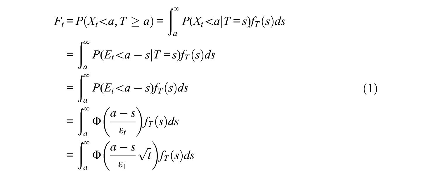
The Probability of an Incorrect Fail
This section will use a classical test theory model to derive a formula that shows how the exam duration affects the expected number of students who fail incorrectly. Assume that the test can be lengthened or shortened without systematically altering the content type or difficulty, thus leaving the true scores the same. That is, the examiner would add or delete test items and change the duration of the examination proportionally. Lord and Novick (1968, Ch. 5) describe this as the model of homogeneous tests with continuous test length. Assume that the test, or a similar test, has been administered previously and that the duration of this administration was
Assume that the examiner estimated from this previous administration the values of

Assume that the cutoff for passing the test is some real number

The correlation between

Note that
The Costs of Measurement and the Costs Measurement Error
This section will incorporate costs in the model. As explained in the introduction, the model will only consider the costs in terms student time. Suppose that the study load of a course is

To find the optimum duration, we have to minimize this in

If the restudy fraction
Example With a Real Exam
In a multiple-choice exam of one of my courses, the nominal study load was 112 hours, the cutoff was
Computation of Expected Number of Incorrectly Failed Students (
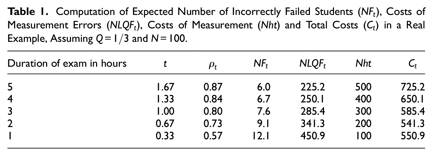
If we consider Table 1 in more detail, we can see what happens. First, consider the reliabilities in column
An obvious weakness in this computation is the unknown value of
Existence of Minimum Costs With Continuous t
This section will show that for continuous
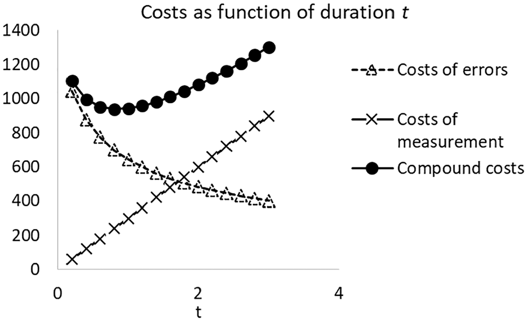
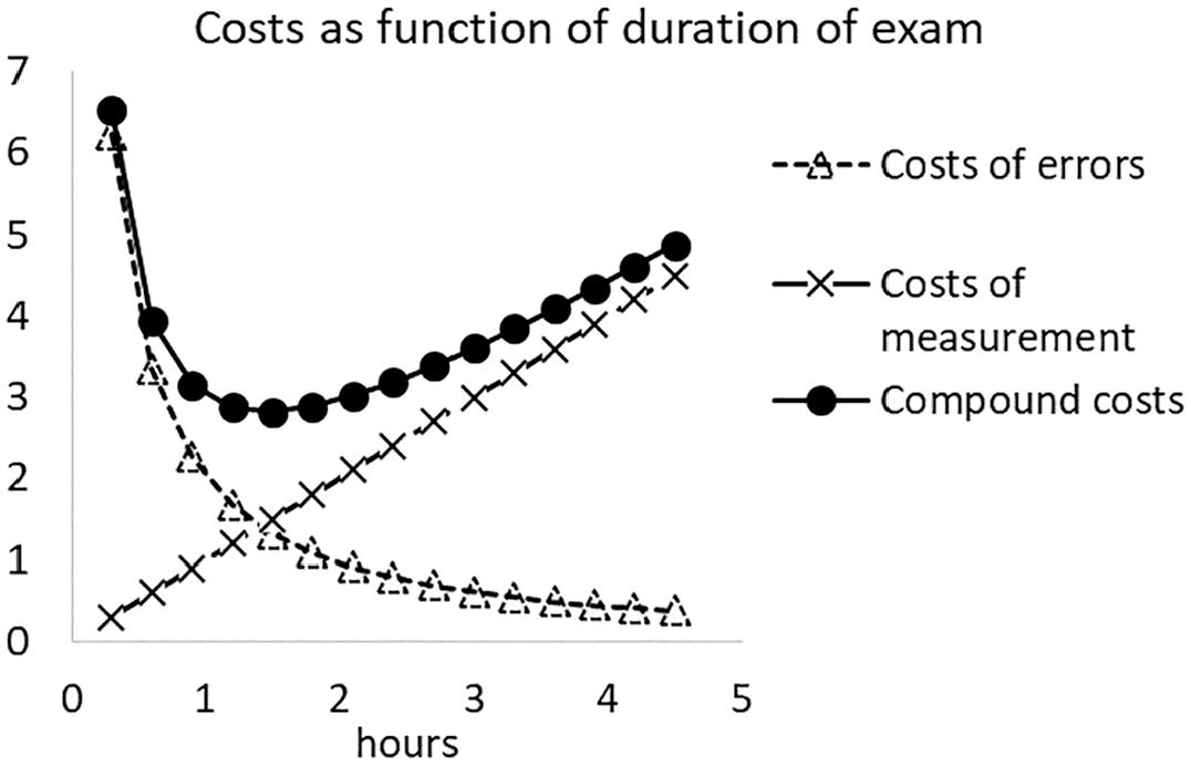
Costs of errors and costs of measurement as a function of the length of the test.
Let us first establish that
Now consider the partial derivative

which is negative for
The second derivative with respect to

For
For the derivative of

We can write the derivative in (2) as

The limit of this for

In sum,
Because

Thus,
Numerical Examples
For the case discussed earlier, with
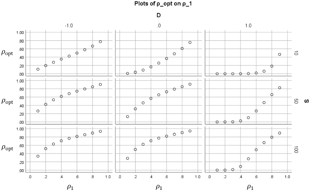
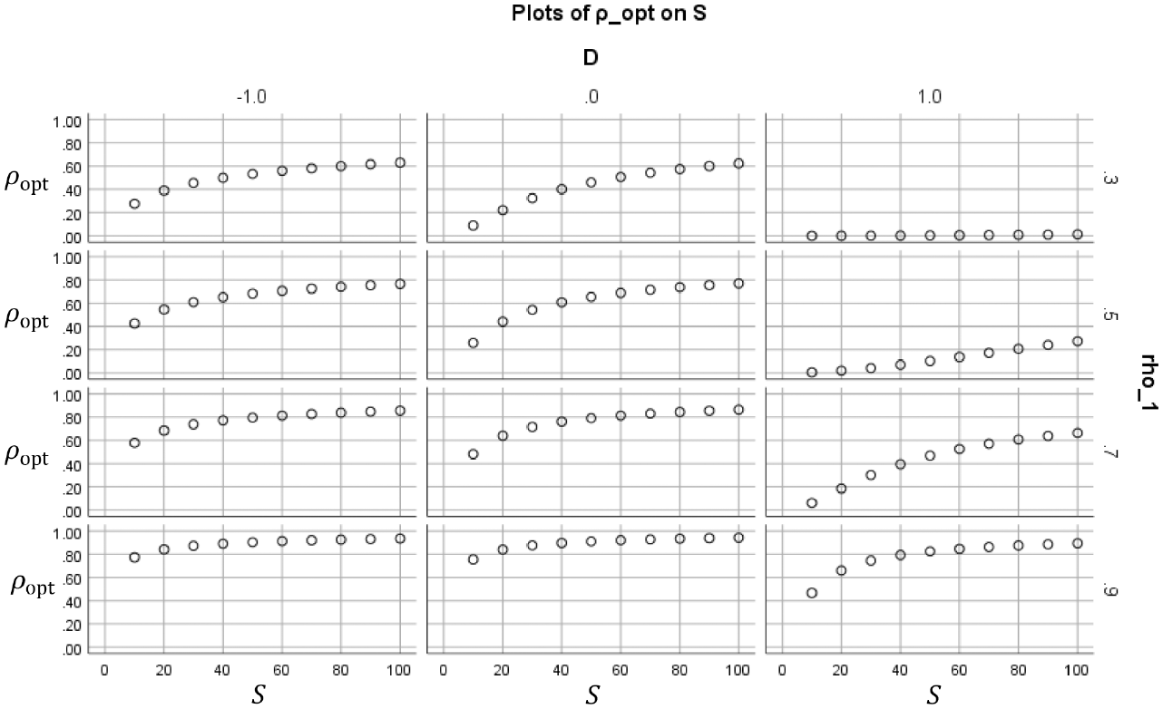
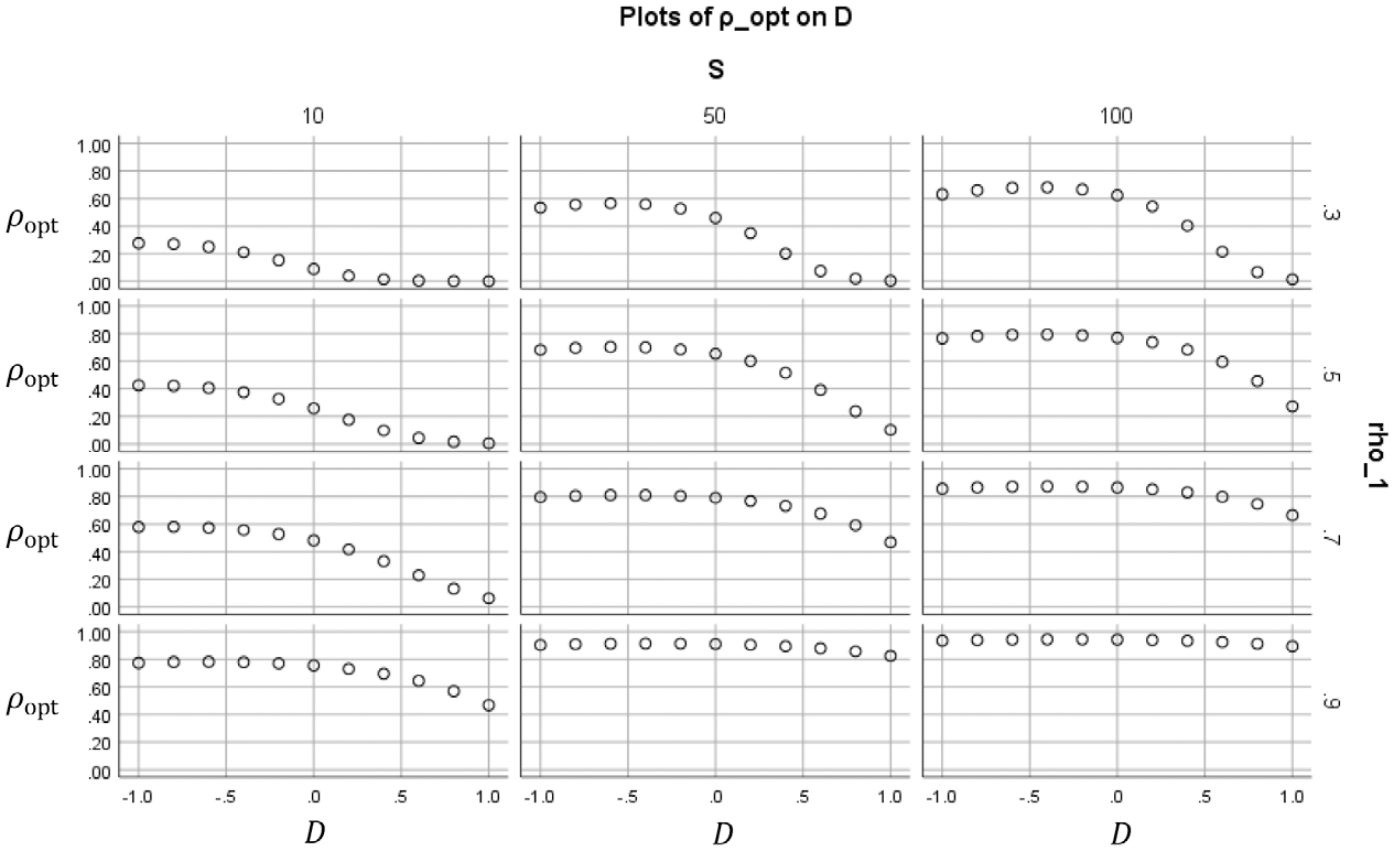
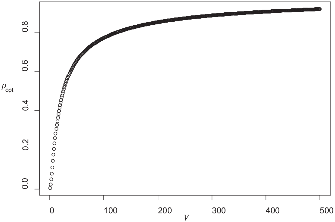
Figures 2 to 5 show how the value of the optimal reliability depends on
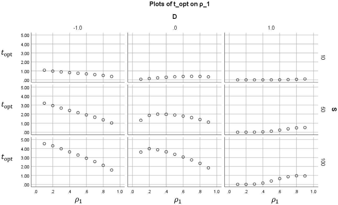
Optimal duration
Optimal reliability
Optimal reliability
Optimal reliability
In Figure 4, each subplot shows for a certain combination of
In Figure 5, each subplot shows for a certain combination of
Analysis of a Special Case
Consider the possibility that the mean of the grades is equal to the cutoff:

(Rose & Smith, 1996, in Weisstein, 2019). Thus

If we write

Although I do not know an analytical solution in

Because of the simplicity of this case, it can be used a default model if one wants to avoid arbitrary assumptions on
Reliability
In the exam of the earlier example, we had
A Model With Score-Dependent Costs
As pointed out by a reviewer, it is possible that the amount of time that a student uses to prepare for the resit depends on the student’s score on the first attempt. This will now be modelled. Assume that, for students who fail the exam, the restudy fraction

if

For a student who incorrectly fails the exam, the expected restudy fraction would be
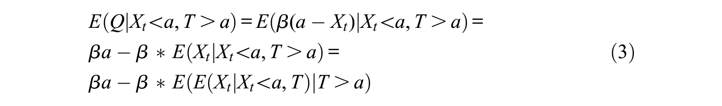
The conditional distribution of

and the expected grade of students who failed incorrectly is


Here, the first two terms do not depend on
As a real data example, consider the case discussed earlier with
Costs of errors and costs of measurement as a function of the exam duration in a case of score-dependent costs.
Sensitivity to Sampling Error
The numerical example was based on empirical estimates of
Discussion
What is the best duration for an exam? How reliable should exam scores be? How is this affected by the study load of the course? In the construction of exams and tests it is often emphasized that they should be reliable. If this were the only criterion, exams should be very long, and in theory even infinitely long. The practical decision whether a certain test is long enough is inevitably partially based on intuitive reasoning and personal experience, since there are hitherto no formal models that justify a less than perfect reliability. This article shows that such models are possible and entail realistic outcomes.
The model created here assumes a classical test theory model, with normally distributed true scores and error scores. From the mean, standard deviation, and reliability of the test, we can compute the probability of erroneous fail on the exam. To quantify the costs of such errors, it was assumed that the students who fail will lose a fraction of the nominal study load because they have to study for the resit. These hours were called the costs of errors. On the other hand, a long test will also consume time from students, and this was called cost of measurement. The compound costs were now defined as the costs of errors plus the costs of measurement. The compound costs were expressed as a function of the test length, and its minimum is easily obtained numerically.
The models make clear that there are many factors contributing to the costs of the exam. If a course is repeated yearly, the examiner can presumably have a reasonable estimate of the values of
What if there is no resit? In that case the model cannot be applied literally. However, one could argue that in this case a student who fails loses the time already spent in the course, which is probably proportional to the study load. Therefore, the same mathematical model would still be appropriate, albeit with a different interpretation of
A limitation of the two models discussed is that students who incorrectly pass the exam (
Overview of Cost Functions.
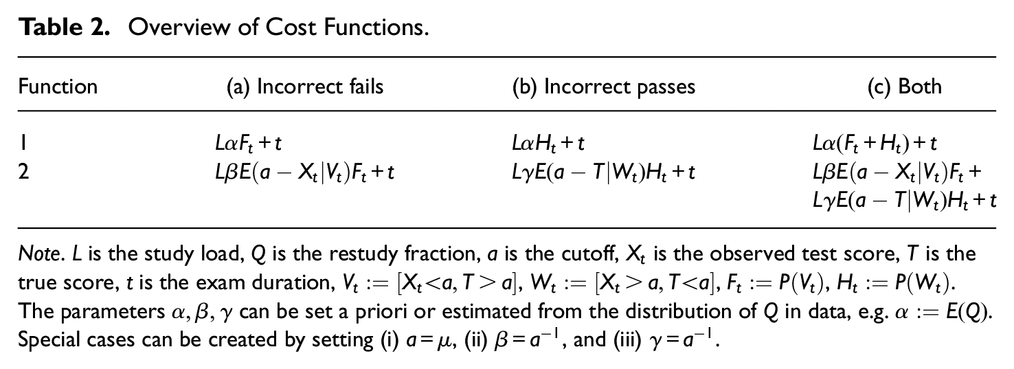
Note.
Another limitation of this study is the usage of the Spearman–Brown formula to predict the reliability under changing test length. It is known that this formula holds if the test items are parallel, but in many cases test items are not parallel. The Spearman–Brown formula holds actually more generally if the items are “essentially parallel” (i.e., essentially tau-eq24 with equal variances), but even this condition is rarely satisfied. The Spearman–Brown formula has also been derived by Raju and Oshima (2005) within an item response theory framework under the assumption that the average item information function does not change if items are added, which is again quite restrictive. However, the Spearman–Brown formula can also be applied to subtests instead of items, where each subtest consists, for example, of 10 items. The assumption of subtests that are approximately essentially parallel is not necessarily unrealistic. The important restriction here is that the items used in long versions of the test should be similar in kind to the items used in short versions of the test. A situation in which this is realistic is if the items are drawn randomly from a large pool of items, particularly if this pool is known to be unidimensional according to an item response theory model. To support this with an example, a simulation was conducted in which items were drawn from a pool of 1,000 items that satisfies the 2-parameter logistic model with discrimination parameters uniformly distributed between 0.5 and 2.5 and difficulty parameters uniformly distributed between −1.5 and 1.5, and these items were used to generate random tests with lengths between 10 and 50 items, in steps of 5 items. For each of these test lengths, 1,000 tests were generated with items randomly drawn from the pool, and the reliability was computed for each test by numerical integration, assuming a standard normal distribution of the latent ability. For test lengths 10, 15, 20, 25, 30, 35, 40, 45, and 50, the average reliabilities were .7417, .8106, .8526, .8775, .8955, .9096, .9199, .9282, and .9349, respectively. These values fit the Spearman–Brown formula almost perfectly: if any of these average reliabilities is predicted from any other one, the error is at most 0.0025. Thus, even though the individual tests might not satisfy the Spearman–Brown formula, the expected reliability across random test versions can still be predicted very well with the Spearman–Brown formula in this example. Consequently, the arguments of the previous sections can be applied here too. It is beyond the scope of this article to determine under which conditions this generalization of the Spearman–Brown formula is appropriate, but a simulation like this can be conducted easily once the item parameters are known.
The Spearman–Brown formula does not account for possible practice and fatigue effects that might influence the reliability if the test length is changed. I do not know of a model that describes the effect of this on the item parameters, but if these effects were strong then this would also invalidate the increasingly popular methods of computerized adaptive testing (e.g., Van der Linden & Glas, 2000), which invariably assume that the ability and item parameters are not affected by the test length.
Thus, for the first time we have now a mathematical tool that allows us to estimate the optimal length of an exam from data of earlier similar exams. The tool is simple and easy to use, but obviously there are some limitations:
The computation requires knowledge of the distribution of
The computation ignored many other costs, such as extra financial costs if failing leads to dropping out of the program, the reputation damage when students with low true scores pass, emotional stress, costs of the school to make longer exams, and so on.
The distribution of item characteristics should remain the same if the test is lengthened or shortened, such that the Spearman–Brown formula is valid. To avoid floor and ceiling effects, it may be better to work with an item response theory model instead of classical test theory.
More detailed and realistic computations may be possible if all these components are added to the model, and the important conclusion from this article is that there is proof of concept.
Footnotes
Declaration of Conflicting Interests
The author(s) declared no potential conflicts of interest with respect to the research, authorship, and/or publication of this article.
Funding
The author(s) received no financial support for the research, authorship, and/or publication of this article.