Sage Journals: Discover world-class research

Abstract

This article disaggregates Donohue and Levitt’s (DL’s) national panel-data models to the state level and shows that high concentrations of teenage abortions in a handful of states drive all of DL’s results in their 2001, 2004, and 2008 articles on crime and abortion. These findings agree with previous research showing teenage motherhood is a major maternal crime factor, whereas unwanted pregnancy is an insignificant factor. Teenage abortions accounted for more than 30% of U.S. abortions in the 1970s, but only 16% to 18% since 2001, which suggests DL’s panel-data models of crime/arrests and abortion were outdated when published. The results point to a broad range of future research involving teenage behavior. A specific means is proposed to reconcile DL with previous articles finding no relationship between crime and abortion.

Keywords

crime teenage abortion hypergeometric distributions panel-data estimation disaggregation

Ten years after Levitt and Dubner’s (2005) bestseller Freakonomics popularized Donohue and Levitt’s (DL; 2001) sensational hypothesis that legalized abortion led to lower crime in the 1990s, the influence of DL continues to grow. DL’s message that “unwantedness leads to high crime” has been spread worldwide by Freakonomics, freakonomics.com, and Freakonomics: The Movie, produced in 2010. Several studies use DL’s data but with alternative specifications and find no relationship between crime and abortion. This study uses DL’s data and methods and shows that, if there is a statistically significant relationship between crime and abortion, it is due to varying concentrations of teenage abortions across states, not unwanted pregnancy.¹

DL’s hypothesis is as follows (Freakonomics): “Legalized abortion led to less unwantedness, unwantedness leads to high crime; legalized abortion, therefore, led to less crime” (p. 139). A more specific statement, implied by the first, is that (DL) “women who have abortions are those most at risk to give birth to children who would engage in criminal activity”² (p. 381). The evidence here shows that these statements are far too general, even based on research prior to DL.

To avoid confusion, this article does not address the question of whether there is a link between crime and abortion. It does not agree with either DL or studies that find no relationship. Instead, DL’s data and methods are extended here to identify the source of the link between crime/arrests and abortion detected in their 2001, 2004, and 2008 data sets, looking beyond DL’s unwantedness explanation to what actually drives their findings. The answer is teenage abortion, which greatly narrows the implications of any relationship between crime and abortion.

The results are important for research across a broad range of disciplines. The major role of teenage abortion implies that much of the crime and abortion research since DL has been misdirected by considering only total abortions in the analyses. A more useful line of inquiry is to explore alternative ways to reduce teen pregnancy, such as Thomas’s (2012) simulation and cost–benefit analyses of three national-level fiscal policies. The sociological and psychological factors that influence teenage behavior are also important. An interesting example in the social context is Manlove, Wildsmith, Welti, Scott, and Ikramullah (2012), who find that, if a young woman’s sexual partner is disengaged from school or work, the odds of a non-marital birth increase, regardless of whether the woman is disengaged. As another example, at the neuropsychological level, Evans-Chase, Kim, and Zhou (2013) observe that “the risk-taking behavior that leads to increases in unwanted pregnancy, . . . during adolescence is nested within the biologically predisposed behavior of sensation seeking” (p. 612). Consistent with these findings, Scott, Rappucci, and Woolard (1995) explain that, from a legal standpoint, teenagers are generally considered less capable of evaluating the consequences of their conduct, such as accurately assessing the level of risk of an unwanted pregnancy.

The results here also point to a simple means to begin resolving questions raised by recent studies that use DL’s data but find no relationship. Specifically, the link between crime and abortion is strongest here when using data from states with distinctly high and low teenage abortion concentrations. The same may prove to be true for earlier studies. If using data from only high and low teenage abortion states reverses the results of the articles described below, then the issue of crime and abortion rests on teenage abortion. If the results are still insignificant, it is reasonable to conclude that there is only a weak link between crime and total abortion (still due to teenage abortion), which is statistically significant mainly under DL’s specifications.

All of DL’s panel-data models are examined here using all three data sets. The national models are disaggregated to the state level to identify the states that drive DL’s results and the states that least support DL’s hypothesis. States with high teenage pregnancy rates and abortion ratios (percent of pregnancies aborted) drive DL’s results and the opposite for states that least support DL. Hypergeometric distributions and DL’s long differences are used to verify the results. The findings agree with previous research showing that (a) teenage motherhood is a major maternal crime factor, (b) unwanted pregnancy is a minor or insignificant factor, and (c) teenage birthrates explain both the increase in U.S. crime in the 1980s and the subsequent decline.³

Several studies challenge DL’s findings. Joyce (2004) compares crime among cohorts born before and after legalized abortion to crime among cohorts unexposed to abortion and finds little evidence that abortion reduces crime. DL (2004) reply by extending Joyce’s analysis to cover the entire lives of the same cohorts and again find that abortion negatively affects crime. Foote and Goetz (2008) report that DL omitted state–year effects in part of their analysis and show that, when this error is corrected and per capita criminal activity is used rather than total activity, DL’s claim regarding crime and abortion vanishes. DL (2008) respond with evidence that, when using a measure of abortion that accounts for cross-state mobility and other timing factors, their crime and abortion conclusions remain.

Lott and Whitley (2007) link the number of abortions when a cohort is born to the crimes later committed by the cohort and find that legalizing abortion is associated with a statistically significant increase in murder. Joyce (2009) uses DL’s data and specifications to analyze age-specific homicide and murder arrest rates and finds no statistically significant relationship with abortion. Moody and Marvell (2010) address the use of control variables and recommend a wide search of alternative variables, testing for significance. Applying the method to DL’s data, they find that imprisonment and police are effective deterrents, but abortion is insignificant.

Anderson and Wells (2008, 2010) use DL’s data in demonstrating improved methods for regression analyses. In the 2008 article, a forward and backward errors framework is used to show that the analyses used in various crime and abortion articles cannot be trusted. In the 2010 article, a Bayesian hierarchical modeling approach to clustered and longitudinal data is used, which shows that there is no empirical link between crime and abortion. Chamlin, Myer, Sanders, and Cochran (2008) use interrupted time-series models to examine birthrates for unmarried women aged 15 to 44 and teenagers (15-19) using data for 1940-2003 from the National Center for Health Statistics. They find no evidence to support DL’s hypothesis, although the time-pattern surrounding 1973 for teenage birthrates conforms more to expectations under DL than those for unmarried women.

Addressing the 1990s declines in crime, Levitt (2004) identifies increased numbers of police, increased imprisonment, the ebbing of the crack epidemic, and legalized abortion as the main drivers. In contrast, Baumer and Wolff (2014) examine trends in individual crimes and their underlying causes, stressing the need to distinguish global, national, and local crime shifts. Also, in reviewing the numerous explanations offered for the declines in crime, they point to many limitations in earlier studies, often due to the lack of data. Baumer and Wolff (2014) credit improved economic perceptions and increased imprisonment, but are skeptical about abortion due to earlier research that discounts early childhood propensity-based explanations.

The Odds of Becoming a Criminal

The main conclusions here are first demonstrated using pre- and post-DL studies and Allan Guttmacher Institute data on abortions by age group. Beginning with pre-DL studies, Rasanen et al. (1999), cited by DL, use the Northern Finland 1966 Birth Cohort data set, which includes 12,058 males, and finds that unwanted pregnancy is a statistically significant but relatively minor maternal crime factor, whereas teenage motherhood is a major factor. Table 1 shows Rasanen et al.’s (p. 859) odds ratios, including only the factors found to be statistically significant, ranked according to the odds ratios for violent crime, then nonviolent crime. The ranking is the same starting with nonviolent crime, except that single-parent family is first. Each factor is estimated while controlling for the others. Unwanted pregnancy ranks fifth, behind mothers who smoke.

Table 1.

Rasanen et al. (1999, p. 859, Table 1) Statistically Significant Odds Ratios.

	Violent crime		Nonviolent crime
Crime fact	Odds ratio	Confidence interval (.95)	Odds ratio	Confidence interval (.95)
Mother’s level of education low	4.3	[1.0, 17.9]	2.0	[1.1, 3.9]
Mother less than 20 years old	2.6	[1.4, 5.0]	1.7	[1.0, 2.7]
Single-parent family	2.4	[1.6, 3.7]	2.5	[1.8, 3.4]
Mother smoked during pregnancy	2.1	[1.3, 3.2]	1.3	[0.9, 1.8]
Mother did not want pregnancy	2.1	[1.4, 3.2]	1.1	[0.8, 1.5]
Not talking at age 1	1.1	[0.7, 1.7]	1.4	[1.0, 1.9]
Not walking at age 1	0.7	[0.4, 1.1]	1.2	[1.0, 1.8]

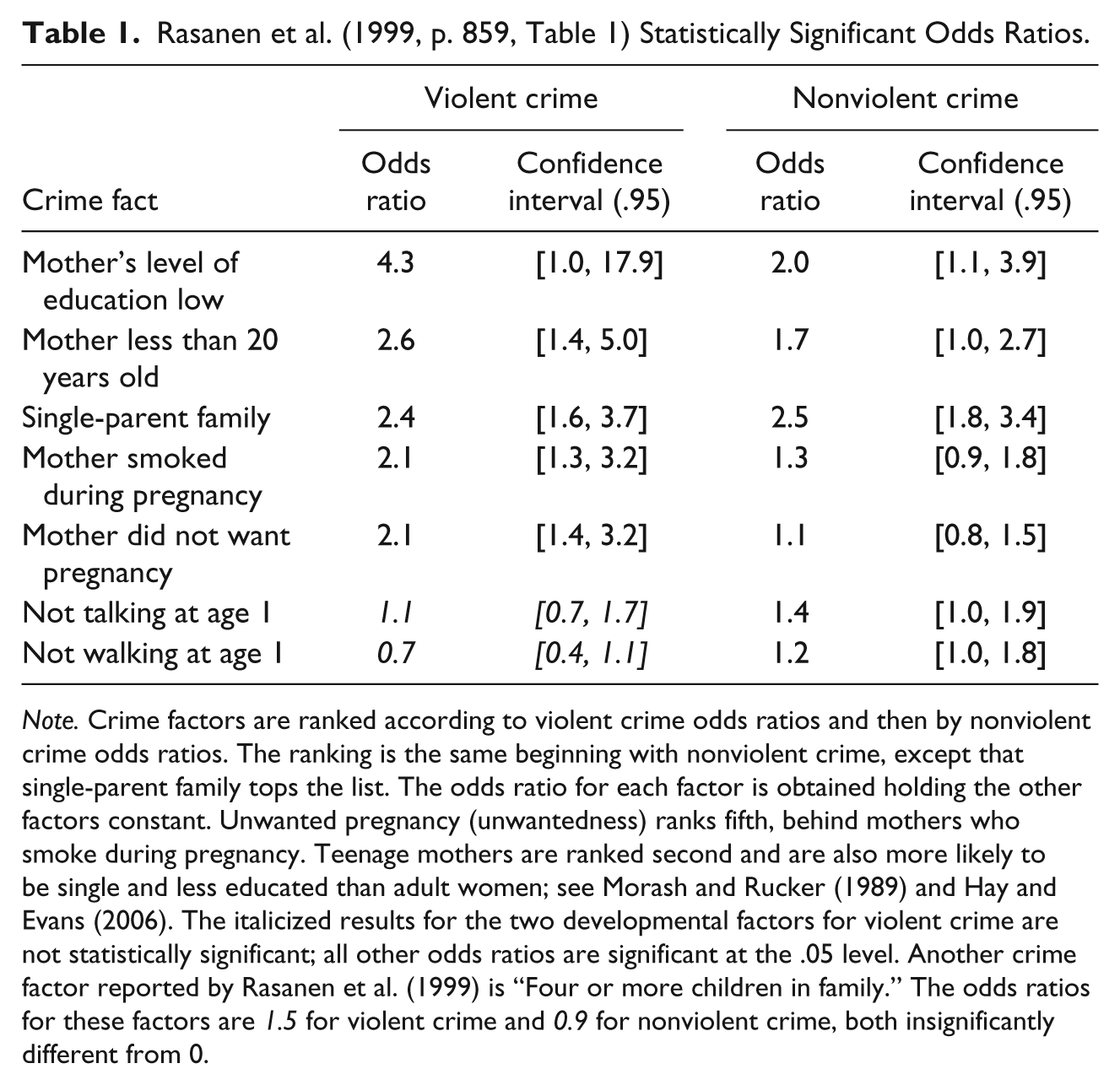
Note. Crime factors are ranked according to violent crime odds ratios and then by nonviolent crime odds ratios. The ranking is the same beginning with nonviolent crime, except that single-parent family tops the list. The odds ratio for each factor is obtained holding the other factors constant. Unwanted pregnancy (unwantedness) ranks fifth, behind mothers who smoke during pregnancy. Teenage mothers are ranked second and are also more likely to be single and less educated than adult women; see Morash and Rucker (1989) and Hay and Evans (2006). The italicized results for the two developmental factors for violent crime are not statistically significant; all other odds ratios are significant at the .05 level. Another crime factor reported by Rasanen et al. (1999) is “Four or more children in family.” The odds ratios for these factors are 1.5 for violent crime and 0.9 for nonviolent crime, both insignificantly different from 0.

Although Rasanen et al.’s (1999) odds ratios are based on Finnish data, their results are used here for four reasons. First, DL (p. 390) rely on Rasanen et al.’s violent crime odds ratio of 2.1 for unwanted pregnancy in stating that unwantedness more than doubles an individual’s likelihood of committing crimes. Second, DL cite Comanor and Phillips (1999), who use data from the National Longitudinal Survey of Youth (NLSY) at Ohio State University and find that adolescents in households with absent fathers are 2.2 times more likely to be charged with a crime, which is close to Rasanen et al.’s odds ratio of 2.4 for violent crime. Third, it is not the magnitudes of Rasanen et al.’s odds ratios that are important here, but their relative magnitudes, which are likely to be similar across countries. Fourth, post-DL studies based on U.S. data reinforce Rasanen et al.’s findings for both teenage motherhood and unwanted pregnancy.

In Table 1, teenage mother is ranked second with an odds ratio of 2.6. However, teenagers are also the most likely candidates for the first and third factors, mother’s education low and single-parent family, having respective odds ratios of 4.3 and 2.4. As confirmation, the pre-DL study by Morash and Rucker (1989) conducts separate analyses using the NLSY and National Survey of Children (NSC) data sets and finds that teenage mothers generally have less education and the biological father is less likely to be in the home. Thus, research based on U.S. data supports combining the first three odds ratios. (The NLSY includes 12,686 U.S. young people. The NSC includes U.S. children born between 1964 and 1969; in the first wave, ages 6 to 12, N = 2,301.)

Given a recent U.S. Census Bureau study by Shattuck and Kreider (2013), which shows that single motherhood is becoming the new norm among adult women in their 20s and 30s, a key result in Table 1 is that the violent crime odds ratio for a single, teenage mother with low education and unwanted pregnancy is roughly 2.5 times that for a single adult mother aged 20 or older with an unwanted pregnancy, and 4.5 times that of a married adult woman with an unwanted pregnancy. During the 1970s, nearly one fourth of U.S. women who had abortions were married. Using U.S. data, unwanted pregnancy has since been found to be an insignificant factor (see below), which would make the disparities in comparative odds ratios even larger.

Rasanen et al.’s (1999) odds ratios agree with the reasons women say they had abortions by age group, as reported by Torres and Forrest (1988). By far, the biggest difference between teenage and adult responses is their own perceived maturity; 68% of teenagers responded as being too immature, but only 21% of women in their 20s and 4% in their 30s. Sizable differences are also reported for not wanting others to know they are pregnant, unready for the responsibility, and cannot afford a baby. Twenty percent of teenagers’ parents wanted them to have an abortion, but only 4% of women in their 20s and 2% in their 30s.

Teenagers know they are unprepared for motherhood and are often under pressure to have an abortion. For teenagers, the adverse social environment in which the child would be raised (possibly resentful and negligent) may be more unwanted than the child itself.⁴ The situation is not as severe for women in their 20s and less for women in their 30s. The reason of change in lifestyle falls from 87% for teenagers to 69% for women in their 30s. Avoiding single parenthood is roughly 50% for all ages. For adult women, the abortion decision appears to be mostly about lifestyle changes, not their ability to raise a child in a positive environment.

In all, the environment likely to be provided by many teenage mothers is consistent with Rasanen et al.’s (1999) maternal crime factors. In contrast, a single or married adult woman is more likely to raise a child in a positive environment, even if from an unwanted pregnancy; that is, a mature and educated mother is unlikely to treat her child as unwanted. Thus, based on the pre-DL studies by Rasanen et al., Morash and Rucker (1989), and Torres and Forrest (1988), adult women are a poor fit for DL’s (p. 381) description of women who have abortions.

The evidence above suggests at least five implications for crime and abortion. First, given that the odds ratios for unwanted pregnancy are no larger than those for mothers who smoke during pregnancy, it is unlikely that reduced unwantedness could account for as much as half of the declines in crime in the 1990s (DL, p. 382). In contrast, states with high teenage abortion rates are more likely to have experienced sizable reductions in crime.

Second, modeling crime across all 50 states, there would need to be a sufficient number of states with high teenage abortion rates and reduced crime, along with other states having low teenage abortion rates and no reduction in crime to obtain statistically significant coefficients; that is, there would need to be variability in the data. Also, the overall percentage of teenage abortions within total abortions would need to be fairly high or there would be no relationship. Indeed, during the 1970s, there were wide variations in teenage abortion and crime rates across states, and teenage abortions accounted for more than 30% of total abortions; see Kost and Henshaw (2012) for teenage abortions and Jones and Kooistra (2011) for total abortions.

Third, with adult abortions accounting for nearly 70% of all abortions, there would need to be a large number of total abortions to reduce crime a small amount. This result is illustrated in Freakonomics (p. 144) using the hypothetical trade-off of 100 fetuses for one person to demonstrate the inefficiency of total abortions in reducing crime.

Fourth, if teenage abortion concentrations within total abortions declined substantially, the coefficient on total abortions would become insignificant. This is effectively illustrated in the panel-data analyses here. By excluding only a handful of states with high teenage pregnancy rates and abortion ratios, the abortion coefficients become insignificant in all of DL’s models.

Fifth, teenage abortions have declined to 16% to 18% of total abortions since 2001. Teenage abortion rates have declined from 43.5 per 1,000 population aged 15 to 19 in 1988 to 22.5 in 2001 (a 48.3% decline) and to 17.8 in 2008 (a 59.1% decline). Thus, it is unlikely that crime data collected starting in 2019 (2001 + 18 years) would again produce statistically significant results for total abortion rates under DL’s specifications; that is, DL’s estimated relationships between crime and abortion were likely obsolete when published.

As further evidence that DL’s statements about unwantedness are unlikely, 46.3% of women who had abortions in 1974 already had at least one child; 29% had two or more children. In 2008, the respective percentages were 61 and 34; see Henshaw and Kost (2008) and Jones, Finer, and Singh (2010) for percentages in intermittent years from 1974 to 2008. Two reasons given for the abortions are the family was considered to be complete and/or an additional child could not be afforded. DL’s hypothesis suggests that a child from an unwanted pregnancy in this situation, if not aborted as a fetus, would be at higher risk of becoming a criminal than the child’s older (wanted) siblings. That seems unlikely, given that all would grow up in the same home environment. However, this raises the issue of family size; that is, having another child might increase the likelihood that all the siblings (especially males) would become criminals.

DL (pp. 391-393) discuss family size and explain that women who prevent larger families by having abortions may indirectly lower criminality for the other children by devoting more parental attention and resources to them. In the end, though, DL (p. 408) note that the effects of family size are likely to be of “second-order” magnitude. Further confirmation is in Rasanen et al. (1999), who include “Four or more children in family” as a factor in their table of odds ratios. The factor has odds ratios of 1.5 for violent crime and 0.9 for nonviolent crime; however, both are statistically insignificant at the .05 level (see footnote to Table 1). Thus, there is good reason to believe that roughly half of all abortions have virtually no impact on crime.

Finally, two post-DL studies effectively eliminate any doubts about teenage motherhood and unwanted pregnancy. First, using NSC data, Hay and Evans (2006) address the question of whether children from unwanted pregnancies are more involved in juvenile delinquency during adolescence and serious crime during adulthood. They find that, during adolescence, unwanted pregnancies account for a statistically significant but modest 1% of the variation in self-reported delinquency, but no evidence is found that the effects extend into adulthood for general or serious crime, confirming the weak, even insignificant, role of unwanted pregnancy.

Second, Hunt (2006) uses International Crime Victims Survey (ICVS) data and shows that teenage birthrates explain why the United States had the highest crime rates of 13 developed countries during the 1980s. For children of teenage mothers, childhood conditions (especially harsh punishment) explain the results. Hunt (2006) also shows that teenage births help explain the subsequent decline in U.S. crime. Thus, the combined evidence in the pre- and post-DL studies described above establish the main conclusions of this study.

National (Aggregate) Panel-Data Results for Crime

The national models in this section serve as bases of comparison for the state-by-state models in the next section. Although DL use generalized least squares (GLS) to adjust for serially correlated errors in all their panel-data models, citing Bhargava, Franzini, and Narendranathan (1982), they do not use the model section procedure in the same article, which is aimed at obtaining efficient estimates.⁵ Applying the procedure, first differences are indicated for all national and state models. Year-fixed effects remain, and DL’s eight control variables are included in all models.⁶

The first two violent and property crime models in Table 2 replicate DL’s (Table IV, p. 404) columns 2 and 4 using the 2001 data and include the control variables: prisoners, police, unemployment rates, income per capita, poverty rates, AFDC (Aid to Families with Dependent Children) generosity, weapons laws, and beer consumption. The second two models use DL’s improved 2004 data set. All four GLS models should be estimated using ordinary least squares (OLS) in first differences based on their d_P statistics, which are from left to right, .418, .539, .436, and .540, all less than the R_PL critical value of .6562 (Bhargava et al., 1982, p. 544).

Table 2.

DL (2001) U.S. National Panel-Data Models of Violent and Property Crime.

	2001 data set		2004 data set
	(Δ)ln(Violent crime per capita)_t	(Δ)ln(Property crime per capita)_t	(Δ)ln(Violent crime per capita)_t	(Δ)ln(Property crime per capita)_t
DL original GLS specification; 50 states plus DC, population weighted
Effective Abortion Rate (×100)_t	−0.129 (−5.33**)	−0.091 (−5.12**)	−0.153 (−5.17**)	−0.111 (−6.04**)
ln(prisoners per capita)_t−1	−0.023 (−0.62)	−0.159 (−4.38**)	−0.030 (−0.68)	−0.160 (−4.39**)
ln(police per capita)_t−1	−0.028 (−0.63)	−0.049 (−1.08)	−0.032 (−0.70)	−0.055 (−1.26)
State unemployment rate_t	0.069 (0.14)	1.310 (3.37**)	0.141 (0.28)	1.465 (3.89**)
ln(state income per capita)_t	0.049 (0.23)	0.084 (0.52)	0.017 (0.08)	.073 (0.46)
Poverty rate (% in poverty)_t	−0.000 (−0.09)	−0.001 (−0.89)	−0.000 (−0.08)	−.001 (−0.78)
AFDC generosity (× 1,000)_t−15	0.008 (1.59)	0.002 (0.43)	0.008 (1.51)	0.001 (0.25)
Shall-issue concealed weapons law_t	−0.004 (−0.30)	0.039 (3.65**)	−0.005 (−0.41)	0.037 (3.50**)
Beer consumption per capita (gallons)_t	0.004 (1.28)	0.004 (1.14)	0.004 (1.08)	0.003 (0.84)
R ²	.942	.992	.944	.992
OLS in first differences, 50 states, unweighted
ΔEffective Abortion Rate_t	−0.156 (−3.75**)	−0.106 (−4.60**)	−0.171 (−3.82**)	−0.107 (−4.40**)
Δln(prisoners per capita)_t−1	−0.037 (−0.65)	−0.044 (−1.27)	−0.036 (−0.64)	−0.045 (−1.29)
Δln(police per capita)_t−1	−0.004 (−0.10)	0.001 (0.04)	−0.005 (−0.12)	−0.001 (−0.02)
ΔState unemployment rate_t	−0.411 (−0.80)	0.809 (2.75**)	−0.372 (−0.72)	0.850 (2.86**)
Δln(state income per capita)_t	0.257 (1.28)	−0.032 (−0.22)	0.254 (1.26)	−0.028 (−0.20)
ΔPoverty rate (% in poverty)_t	0.002 (0.94)	0.001 (0.58)	0.002 (0.94)	0.001 (0.56)
ΔAFDC generosity (× 1,000)_t−15	0.003 (0.48)	0.000 (0.03)	0.003 (0.46)	−0.000 (−0.00)
ΔShall-issue concealed weapons law_t	−0.017 (−1.17)	0.008 (0.50)	−0.017 (−1.20)	0.008 (0.51)
ΔBeer consumption per capita (gallons)_t	−0.000 (−0.04)	−0.000 (−0.06)	−0.000 (−0.01)	0.000 (0.01)
R ²	.265	.227	.266	.223
DL original GLS specification; 36 states, population weighted^a
Effective Abortion Rate (×100)_t	−0.093 (−1.35)	−0.046 (−1.55)	−0.070 (−1.06)	−0.028 (−0.84)
R ²	.456	.973	.457	.931
OLS in first differences, 36 states, unweighted^a
ΔEffective Abortion Rate (×100)_t	−0.082 (−1.11)	−0.046 (−1.51)	−0.096 (−1.30)	−0.031 (−0.93)
R ²	.267	.215	.268	.213

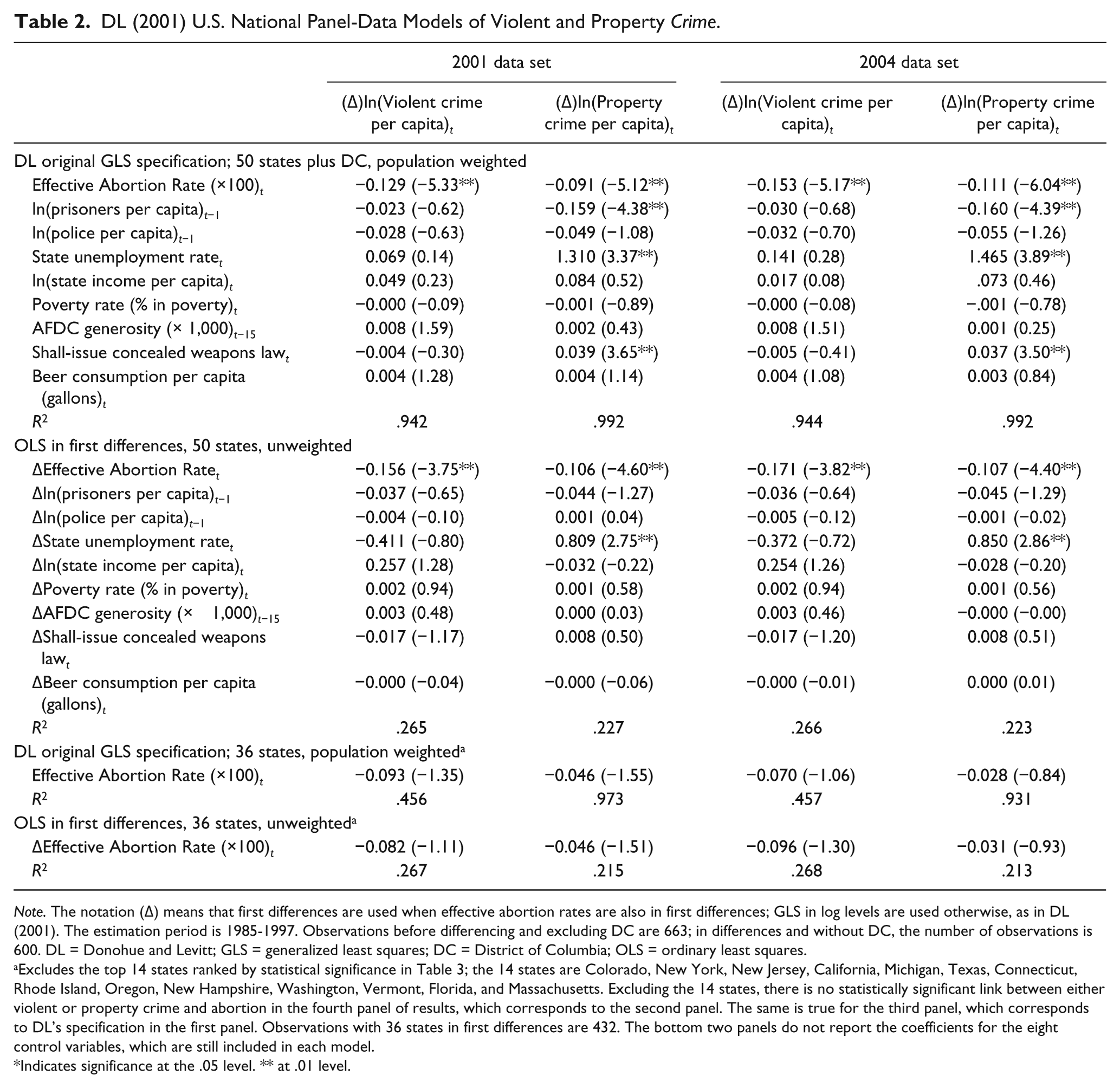
Note. The notation (Δ) means that first differences are used when effective abortion rates are also in first differences; GLS in log levels are used otherwise, as in DL (2001). The estimation period is 1985-1997. Observations before differencing and excluding DC are 663; in differences and without DC, the number of observations is 600. DL = Donohue and Levitt; GLS = generalized least squares; DC = District of Columbia; OLS = ordinary least squares.

Excludes the top 14 states ranked by statistical significance in Table 3; the 14 states are Colorado, New York, New Jersey, California, Michigan, Texas, Connecticut, Rhode Island, Oregon, New Hampshire, Washington, Vermont, Florida, and Massachusetts. Excluding the 14 states, there is no statistically significant link between either violent or property crime and abortion in the fourth panel of results, which corresponds to the second panel. The same is true for the third panel, which corresponds to DL’s specification in the first panel. Observations with 36 states in first differences are 432. The bottom two panels do not report the coefficients for the eight control variables, which are still included in each model.

Indicates significance at the .05 level. ** at .01 level.

The differenced models in the second panel of Table 2 are the focus of the exercise in the next section. These models remove population weighting so that the aggregate and corresponding disaggregate models do not emphasize one state’s data over another. The District of Columbia (DC) is also removed, given an initial state-by-state model that shows DC has no significant effect. Without population weighting and excluding DC, the aggregate coefficients have lower t statistics, but remain significant at the .01 level. Thus, the coefficient estimates in the second panel are efficient and suitable for disaggregation to determine the states that drive DL’s results. (To save space, Table 2 also includes models in the third and fourth panels that are referenced in the next section; coefficients are not shown for the eight control variables still included.)

State-by-State (Disaggregate) Panel-Data Results for Crime

The specification of each state-by-state model is the same as the corresponding model in the second panel of Table 2, except that separate coefficients are estimated for each state. This is accomplished by creating 50 column vectors of effective abortion rates by multiplying the single vector of values used in each of the four models in the second panel of Table 2 by the state-fixed effects dummies. In this way, separate slope coefficients are obtained for all 50 states. The estimation of separate state coefficients is not new; see, for example, Marvell (2010), Defina and Arvanites (2002), and Marvell and Moody (1998).

The 50 states are then rank-ordered by coefficient significance levels for both violent and property crime and 2001 and 2004 data sets. The highest rank of 50 is assigned in each case to the state with the largest negative t statistic, declining to the rank of 1 having the largest positive t statistic. The 50 states are then ranked overall by averaging the four individual ranks. Table 3 lists the states ranked-ordered according to each state’s average rank in the last column. This approach is simple and verified in multiple ways as an effective way to rank states having the strongest and weakest relationships between crime and abortion.

Table 3.

Disaggregate Models in First Differences, 50 States Ranked by Statistical Significance.

	2001 data set				2004 data set				Overall rank
	ΔViolent effective abortion rate_t	Rank	ΔProperty effective abortion rate_t	Rank	ΔViolent effective abortion rate_t	Rank	ΔProperty effective abortion rate_t	Rank	Overall rank
Colorado	−0.254 (−1.50)	49	−0.147 (−2.15)	47	−0.282 (−1.28)	49	−0.117 (−1.38)	47	48.00
New York	−0.127 (−1.66)	50	−0.073 (−1.67)	42	−0.171 (−1.51)	50	−0.082 (−1.50)	49	47.75
New Jersey	−0.113 (−0.98)	47	−0.103 (−2.59)	50	−0.101 (−0.80)	47	−0.062 (−1.36)	46	47.50
California	−0.061 (−0.62)	43	−0.106 (−2.27)	49	−0.075 (−0.57)	42	−0.083 (−1.49)	48	45.50
Michigan	−0.193 (−1.25)	48	−0.106 (−1.71)	43	−0.218 (−1.05)	48	−0.072 (−0.91)	41	45.00
Texas	−0.128 (−0.59)	42	−0.221 (−2.23)	48	−0.149 (−0.55)	40	−0.173 (−1.51)	50	45.00
Connecticut	−0.117 (−0.71)	44	−0.094 (−2.00)	44	−0.119 (−0.66)	44	−0.052 (−0.92)	42	43.50
Rhode Island	−0.092 (−0.57)	41	−0.153 (−2.14)	46	−0.106 (−0.51)	38	−0.120 (−1.36)	45	42.50
Oregon	−0.154 (−0.88)	46	−0.079 (−0.57)	34	−0.158 (−0.73)	46	−0.024 (−0.17)	35	40.25
New Hampshire	−0.147 (−0.51)	37	−0.160 (−1.49)	41	−0.178 (−0.54)	39	−0.119 (−0.98)	43	40.00
Washington	−0.056 (−0.50)	34	−0.066 (−1.07)	38	−0.073 (−0.46)	35	−0.048 (−0.58)	39	36.50
Vermont	−0.067 (−0.24)	30	−0.182 (−1.11)	39	−0.101 (−0.48)	36	−0.180 (−0.91)	40	36.25
Florida	−0.061 (−0.47)	33	−0.067 (−1.20)	40	−0.075 (−0.44)	34	−0.039 (−0.57)	38	36.25
Massachusetts	−0.015 (−0.12)	28	−0.112 (−2.13)	45	−0.019 (−0.13)	27	−0.079 (−1.34)	44	36.00
Maine	−0.127 (−0.50)	35	−0.104 (−0.29)	28	−0.186 (−0.57)	41	−0.048 (−0.34)	37	35.25
Illinois	−0.025 (−0.14)	29	−0.052 (−0.83)	36	−0.041 (−0.19)	29	−0.012 (−0.16)	34	32.00
Georgia	−0.092 (−0.53)	38	−0.013 (−0.13)	25	−0.113 (−0.50)	37	0.027 (0.24)	25	31.25
Wyoming	−0.423 (−0.55)	40	0.048 (0.14)	14	−0.256 (−0.58)	43	0.095 (0.51)	17	28.50
Wisconsin	0.112 (0.38)	17	−0.095 (−0.94)	37	0.082 (0.23)	18	−0.033 (−0.28)	36	27.00
Ohio	−0.079 (−0.41)	31	−0.008 (−0.12)	24	−0.095 (−0.39)	31	0.038 (0.42)	19	26.25
Kansas	0.001 (0.01)	24	−0.019 (−0.29)	27	−0.035 (−0.10)	25	0.023 (0.17)	27	25.75
Kentucky	−0.275 (−0.50)	36	−0.005 (−0.03)	21	−0.284 (−0.43)	32	0.103 (0.57)	14	25.75
Missouri	−0.164 (−0.54)	39	0.014 (0.10)	15	−0.134 (−0.44)	33	0.068 (0.54)	16	25.75
Virginia	0.045 (0.30)	20	−0.033 (−0.52)	33	0.025 (0.14)	22	0.009 (0.13)	28	25.75
Alabama	−0.230 (−0.77)	45	0.080 (0.72)	6	−0.240 (−0.70)	45	0.134 (1.07)	6	25.50
Iowa	0.215 (0.33)	19	−0.114 (−0.60)	35	0.167 (0.27)	16	−0.024 (−0.13)	32	25.50
Montana	−0.186 (−0.42)	32	0.028 (0.09)	17	−0.173 (−0.35)	30	0.117 (0.30)	23	25.50
Arizona	−0.007 (−0.03)	26	−0.017 (−0.11)	23	−0.036 (−0.12)	26	0.037 (0.23)	26	25.25
Idaho	0.001 (0.00)	25	−0.053 (−0.21)	26	−0.031 (−0.04)	23	0.061 (0.25)	24	24.50
Nevada	0.081 (0.43)	15	−0.019 (−0.36)	29	−0.047 (−0.21)	19	0.003 (0.05)	31	23.50
Maryland	−0.012 (−0.10)	27	0.003 (0.06)	18	−0.016 (−0.13)	28	0.027 (0.55)	15	22.00
Oklahoma	0.150 (0.48)	13	−0.052 (−0.40)	30	0.123 (0.31)	13	0.016 (0.10)	29	21.50
New Mexico	0.116 (0.44)	14	−0.043 (−0.48)	32	0.098 (0.30)	14	0.044 (0.37)	21	20.50
Alaska	0.330 (0.92)	8	−0.111 (−0.43)	31	0.271 (0.72)	8	−0.035 (−0.15)	33	20.00
Hawaii	0.048 (0.23)	22	0.013 (0.16)	13	0.037 (0.15)	21	0.048 (0.51)	18	18.50
Delaware	0.172 (0.74)	10	−0.011 (−0.09)	22	0.131 (0.53)	10	0.011 (0.09)	30	18.00
Minnesota	0.093 (0.35)	18	−0.002 (−0.01)	19	0.058 (0.17)	12	0.058 (0.42)	20	17.25
Louisiana	0.003 (0.01)	23	0.080 (0.50)	8	−0.028 (−0.06)	24	0.154 (0.89)	8	15.75
Arkansas	0.121 (0.28)	21	0.108 (0.56)	7	0.069 (0.16)	20	0.173 (0.98)	7	13.75
Pennsylvania	0.093 (0.54)	12	0.006 (0.09)	16	0.079 (0.36)	13	0.048 (0.62)	13	13.50
North Dakota	0.491 (1.26)	3	−0.004 (−0.02)	20	0.565 (0.72)	7	0.101 (0.31)	22	13.00
Indiana	0.359 (0.84)	9	0.033 (0.27)	10	0.221 (0.63)	9	0.096 (0.84)	9	9.25
North Carolina	0.077 (0.42)	16	0.087 (1.17)	1	0.058 (0.25)	17	0.131 (1.49)	1	8.75
Utah	0.864 (1.13)	7	0.164 (0.42)	9	0.668 (0.72)	6	0.324 (0.79)	11	8.25
South Carolina	0.228 (0.69)	11	0.082 (0.81)	5	0.171 (0.50)	11	0.123 (1.13)	5	8.00
Nebraska	0.505 (1.31)	2	0.031 (0.26)	11	0.565 (1.04)	1	0.118 (0.68)	12	6.50
West Virginia	0.913 (1.39)	1	0.036 (0.16)	12	0.439 (0.96)	3	0.132 (0.82)	10	6.50
South Dakota	0.680 (1.23)	5	0.185 (0.88)	4	0.518 (0.86)	5	0.261 (1.24)	4	4.50
Tennessee	0.228 (1.25)	4	0.089 (1.07)	3	0.231 (0.88)	4	0.147 (1.38)	3	3.50
Mississippi	1.025 (1.22)	6	0.482 (1.13)	2	0.620 (1.02)	2	0.441 (1.49)	2	3.00

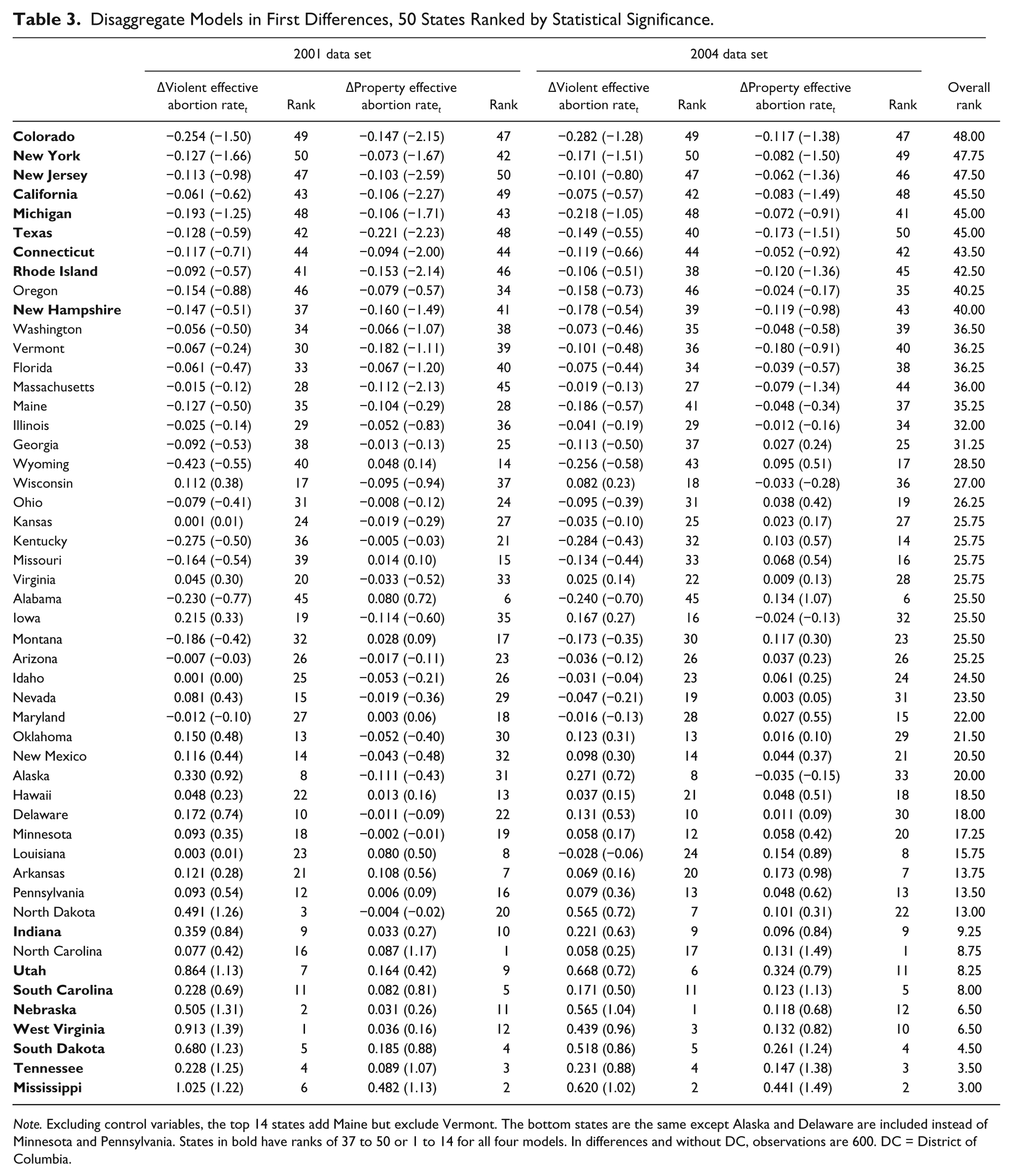
Note. Excluding control variables, the top 14 states add Maine but exclude Vermont. The bottom states are the same except Alaska and Delaware are included instead of Minnesota and Pennsylvania. States in bold have ranks of 37 to 50 or 1 to 14 for all four models. In differences and without DC, observations are 600. DC = District of Columbia.

Although Table 3 models are based on 600 observations, the coefficients are effectively estimated with 12 observations; thus, few are significant at the .05 level. What is known is that the collective effect of the 50 coefficients produces the single coefficients in the second panel of Table 2 and that the t statistics should reflect the relative significance of each state’s impact on violent and property crime. To verify the rank-ordered results, hypergeometric distributions are used. The most important finding in this exercise, as discussed below, is that there is a near one-to-one correspondence between ranked significance and ranked teenage abortion concentrations.

A practical way to define high- and low-impact states is to determine the number of top-ranked states necessary to make DL’s results statistically insignificant, and then choose the same number of states from the lowest ranks. Excluding the top 14 states causes all four abortion coefficients in the second panel of Table 2 to be insignificant at the .05 level, as shown in the fourth panel. DL’s original estimates in the first panel also become insignificant, as shown in the third panel. The 14 states are, in order, Colorado, New York, New Jersey, California, Michigan, Texas, Connecticut, Rhode Island, Oregon, New Hampshire, Washington, Vermont, Florida, and Massachusetts. The states include high- and low-population states, high- and low-crime states and, as shown in the next section, both midrange- and high-abortion states. Although the 14 states account for 47.2% of U.S. population, which is relevant for the models in the first panel of Table 2, the states represent only 28% of the data for the models in the second panel.

Examining the rank-ordered states in Table 3, it is expected that the states’ ranks will be similar for violent and property crime in each data set, as criminal activity in both categories should be affected by aborting fetuses more likely to become criminals. The rank orders should be even more closely related for violent and property crime across the 2001 and 2004 data sets.

Hypergeometric distributions are a useful way to evaluate similarities in the lists of states. Comparing the first two columns of Table 3, the parameters of the hypergeometric distribution are 50 members (states), 14 successes (top 14 states based on abortion significance for violent crime), and a “random” sample without replacement of size 14 (top 14 states based on abortion significance for property crime). There are nine successes (matching states) in the two lists, indicated in bold. The probability of nine successes out of 14 occurring randomly in a sample of 14 is .00080 (.08%). The probability of nine or more is .00086, as the probability of 10 is .00006 and the probabilities of 11 to 14 are each zero to five decimal places (the level of precision of the software). Thus, the two lists are not random, but closely related.

Doing the same for violent and property crime using the 2004 data set, the number of matching states is again nine. Comparing violent crime across the 2001 and 2004 data sets, the relatedness of the lists is even higher, with 10 of 14 matches, and for property crime, 13 matches. Thus, the ranking of states by significance produces similar lists of states that drive violent and property crime in both data sets. The nine states in bold appear in the top 14 states of all four lists.

Again using the last column of Table 3, the bottom 14 states are, in order of least significance, Mississippi, Tennessee, South Dakota, West Virginia, Nebraska, South Carolina, Utah, North Carolina, Indiana, North Dakota, Pennsylvania, Arkansas, Louisiana, and Minnesota. Eight of the bottom nine states in the first column (in bold) appear in all four bottom 14 lists. Comparing violent and property crime for 2001, the probability of eight or more matches with ranks of 1 to 14 occurring in a random sample of 14 is .00710. Comparing violent and property crime lists with the 2004 data, nine states are common. Comparing bottom 14 violent crime lists across the two data sets, there are 10 matches. Comparing property crime lists across data sets, there are 11 matches. Thus, the bottom 14 states across the different lists are also closely related.

Confirming other expectations, removing the 14 bottom-ranked states from the models in the second panel of Table 2, the coefficients are smaller in absolute value, but still significant at the .05 level. Estimating the models with the 22 middle states, the four t statistics are between −.29 and .47. Finally, estimating the four models without the 22 middle states, the coefficients (t statistics) for abortion are, in order, −.234 (−5.47), −.147 (−5.09), −.274 (−5.77) and −.170 (−6.04). Thus, including only the 14 highest and lowest ranked states produces the strongest results.⁷

DL’s Long Differences

DL’s long differences also support the top and bottom 14 states identified above. Figures 1 and 2 are DL’s long difference graphs for violent and property crime, respectively. The horizontal axes measure the changes in effective abortion rates between 1985 and 1997, and the vertical axes show changes in logged crime rates between the same 2 years. For each crime category, the top 14 states are indicated in parenthesis ( ) and the bottom 14 states in brackets [ ]. The top 14 states appear in the lower-right and lower-middle regions of the graphs. The bottom 14 states are mostly in the upper-left regions, the separation being obvious with few exceptions.

Figure 1.

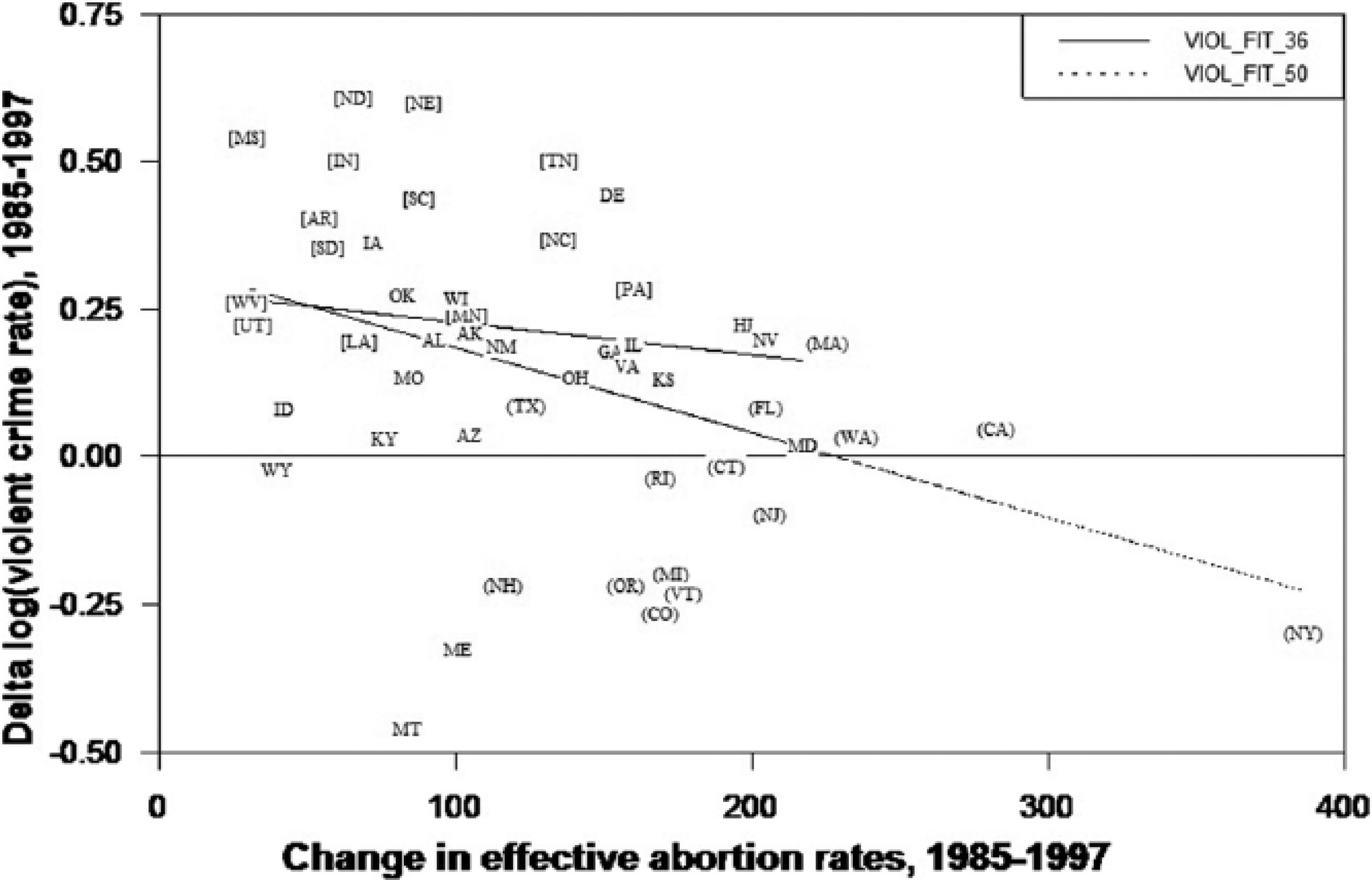
Violent crime long differences with fitted values for 36 and 50 states.

Figure 2.

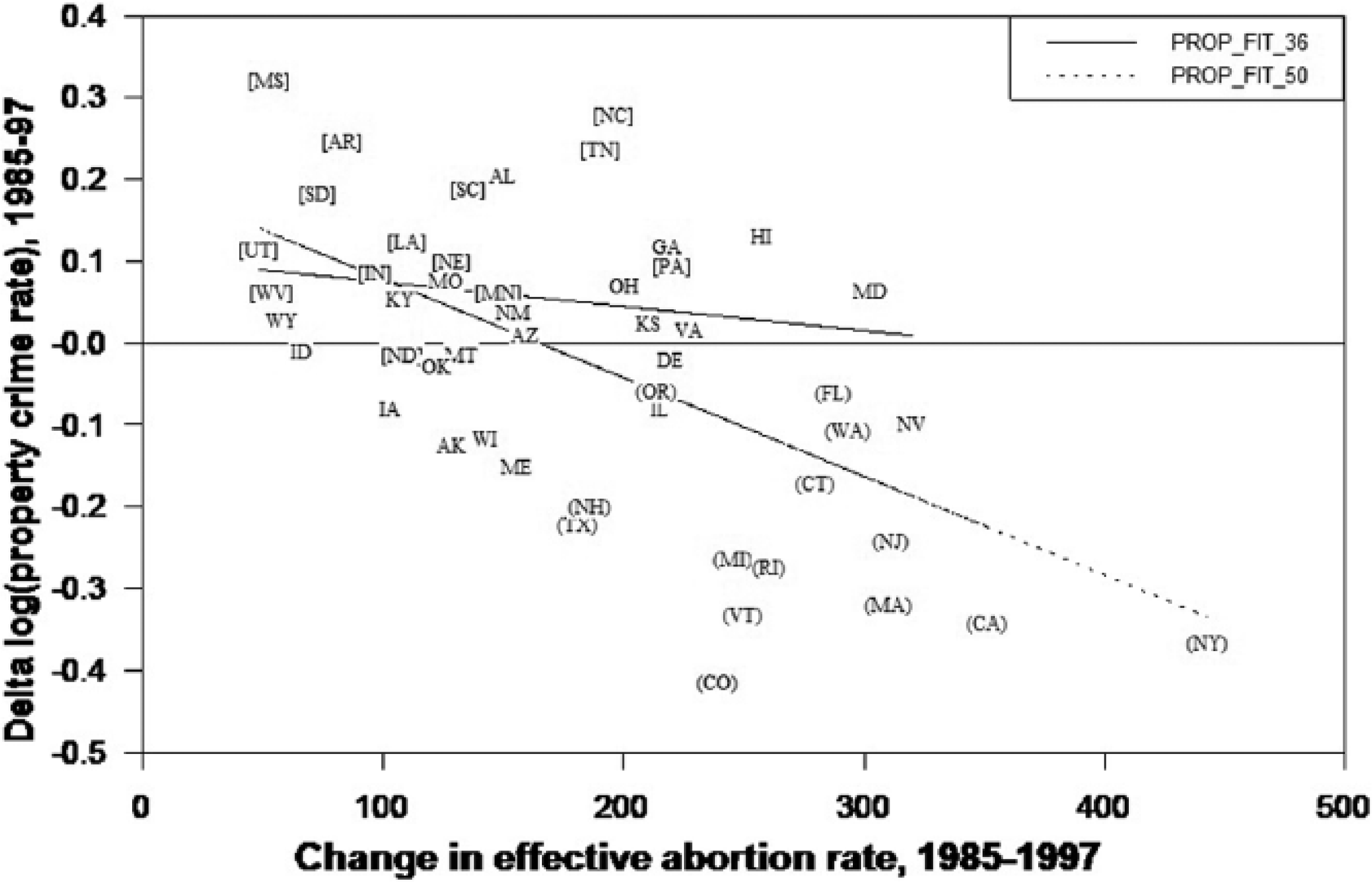
Property crime long differences with fitted values for 36 and 50 states.

For the fitted values in Figures 1 and 2, the violent crime t statistic for the long-differenced effective abortion rate coefficient is −3.12, and for property crime −5.19. Excluding the top 14 states, the respective t statistics are −.74 and −1.05. Using the 2004 data and excluding the top 14 states, the violent crime t statistic declines from −2.92 to −1.21, and for property crime, −4.56 to −1.16. Thus, like the panel-data results, without the top 14 states, there is no longer a significant link between crime and abortion. Also as before, excluding the bottom-ranked states in Figures 1 and 2 reduces the t statistics, but the coefficients remain significant at .05. Excluding both top- and bottom-ranked states, the coefficients for the 22 middle states are all positive and insignificant. Including only the top and bottom 14 states, the t statistics are −4.27 and −5.90. Thus, the results parallel the panel-data models, but are visually apparent.

Although Figures 1 and 2 are fairly simplistic, they offer important information about the relationship between crime and abortion. Several states need explanation, such as Tennessee and Michigan. Michigan’s change in violent crime effective abortion rates is not much larger than Tennessee’s, yet Tennessee violent crime increased 50% between 1985 and 1997, whereas Michigan violent crime decreased 22%. A similar comparison applies to property crime. Other states also need explanation, such Texas, North Carolina, and Colorado. The low-population states of New Hampshire, Delaware, and Vermont also stand out, but these states are marginalized throughout DL by population weighting.

It is important to notice that the states that drive the relationships between crime and abortion are not only states with large increases in effective abortion rates. In Figure 1, six of the top 14 states, New Hampshire, Oregon, Michigan, Vermont, Colorado, and Rhode Island, have increases in effective abortion rates that are less than half that of New York and no larger than those for many other states, yet the six states experienced large decreases in crime. As shown in the next section, these states have large teenage abortion rates and ratios.

State-by-State, Teenage Abortion and Crime

Teenage pregnancy and abortion data show that the difference between the 14 states that underpin DL’s hypothesis and the bottom 14 states are teenage pregnancy rates and abortion ratios. The abortion ratio is the abortion rate divided by the sum of the abortion rate and birthrate, all rates being the number of events per 1,000 women aged 15 to 19. Because some states have high teenage abortion ratios but low teenage pregnancy rates (e.g., Iowa, Nebraska, and Wisconsin) and, therefore, no expected relationship with crime, state abortion ratios are weighted by the fraction (birthrate + abortion rate)_state/(birthrate + abortion rate)_{50-state mean}. Thus, the highest weighted abortion ratios are in states with high teenage pregnancy rates and high abortion ratios.

Table 4 presents teenage weighted abortion ratios for each of the top- and bottom-ranked 14 states for 6 intermittent years between 1988 and 2008. For most years, the ratios for the top 14 states are roughly double those for the bottom 14. The most noticeable exceptions are for Texas in the top 14 and North Carolina in the bottom 14, as indicated in the last panel showing overlapping weighted teenage abortion ratios. The gap in teenage weighted abortion ratios persisted for 21 years, 1988 to 2008, even as the ratios declined substantially over time.

Table 4.

Teenage (15-19) Weighted Abortion Ratios for States Ranked by Significance Levels.^a

	1988	1992	1996	2000	2005	2008	Range	Means
Top-ranked 14 states
California	.80	.71	.60	.54	.47	.43	.43-.80	.59
Colorado	.44	.42	.39	.29	.29	.29	.29-.44	.35
Connecticut	.65	.50	.49	.45	.47	.47	.45-.65	.51
Florida	.58	.47	.52	.51	.44	.40	.40-.58	.49
Massachusetts	.59	.42	.48	.39	.35	.31	.31-.59	.42
Michigan	.55	.42	.39	.36	.35	.32	.32-.55	.40
New Hampshire	.48	.25	.27	.26	.20	.16	.16-.48	.27
New Jersey	.67	.51	.65	.72	.69	.54	.51-.72	.63
New York	.68	.67	.67	.69	.73	.67	.67-.73	.68
Oregon	.48	.36	.35	.38	.29	.29	.29-.48	.36
Rhode Island	.40	.39	.40	.35	.36	.32	.32-.40	.37
Texas	.35	.29	.31	.26	.24	.20	.20-.35	.27
Vermont	.41	.29	.29	.21	.27	.23	.21-.41	.29
Washington	.53	.47	.39	.39	.36	.34	.34-.53	.41
Means	.54	.44	.44	.41	.39	.35	.35-.55	43
Bottom-ranked 14 states
Arkansas	.30	.26	.21	.23	.15	.18	.15-.30	.22
Indiana	.28	.25	.25	.18	.16	.14	.14-.28	.21
Louisiana	.26	.17	.20	.17	.16	.25	.16-.26	.20
Minnesota	.33	.21	.21	.20	.18	.18	.18-.33	.22
Mississippi	.18	.21	.21	.24	.20	.22	.20-.24	.21
Nebraska	.30	.23	.19	.18	.15	.13	.13-.30	.19
North Carolina	.50	.38	.33	.33	.27	.25	.25-.50	.35
North Dakota	.20	.15	.13	.12	.13	.14	.12-.20	.15
Pennsylvania	.38	.30	.27	.26	.26	.32	.26-.38	.30
South Carolina	.37	.26	.25	.26	.29	.25	.25-.37	.28
South Dakota	.17	.16	.13	.11	.11	.09	.09-.17	.13
Tennessee	.35	.27	.24	.24	.22	.22	.22-.35	.26
Utah	.17	.10	.09	.09	.11	.11	.09-.17	.11
West Virginia	.19	.18	.16	.15	.15	.14	.14-.19	.16
Means	.28	.22	.21	.20	.18	.19	.17-.29	.21
Overlapping weighted abortion ratios between top 14 and bottom 14 states^b
Top 14 states with ratios in bottom 14 range	Texas	Texas/New Hampshire	New Hampshire	New Hampshire /Vermont	Texas/New Hampshire	Texas/New Hampshire /Vermont
Bottom 14 states with ratios in top 14 range	North Carolina	North Carolina/Pennsylvania	North Carolina	North Carolina/Pennsylvania	North Carolina/South Carolina	North Carolina/Pennsylvania/South Carolina

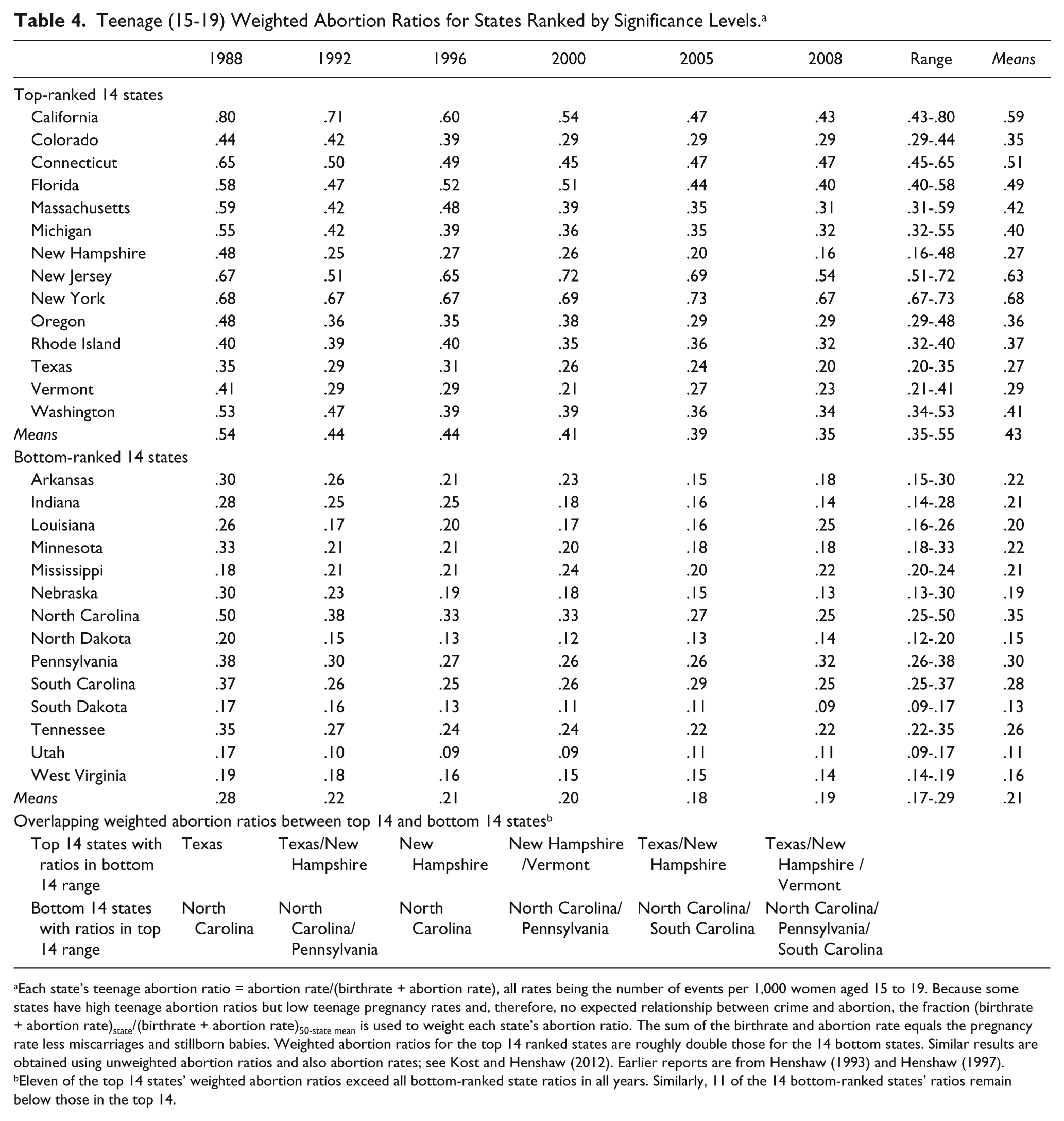
Each state’s teenage abortion ratio = abortion rate/(birthrate + abortion rate), all rates being the number of events per 1,000 women aged 15 to 19. Because some states have high teenage abortion ratios but low teenage pregnancy rates and, therefore, no expected relationship between crime and abortion, the fraction (birthrate + abortion rate)_state/(birthrate + abortion rate)_{50-state mean} is used to weight each state’s abortion ratio. The sum of the birthrate and abortion rate equals the pregnancy rate less miscarriages and stillborn babies. Weighted abortion ratios for the top 14 ranked states are roughly double those for the 14 bottom states. Similar results are obtained using unweighted abortion ratios and also abortion rates; see Kost and Henshaw (2012). Earlier reports are from Henshaw (1993) and Henshaw (1997).

Eleven of the top 14 states’ weighted abortion ratios exceed all bottom-ranked state ratios in all years. Similarly, 11 of the 14 bottom-ranked states’ ratios remain below those in the top 14.

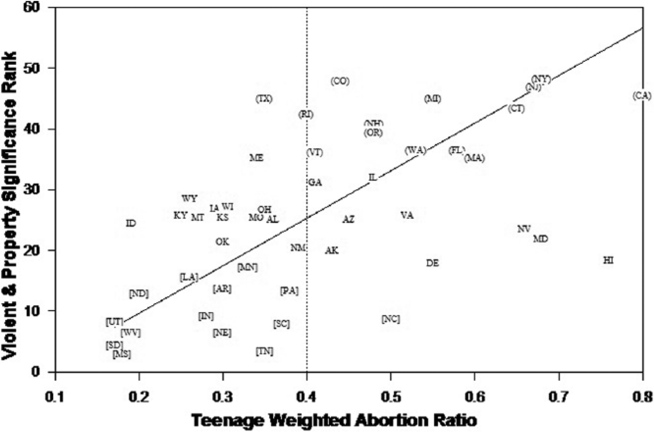
Figure 3 shows the same teenage weighted abortion ratios for 1988 as in Table 4, but for all 50 states versus rank-ordered significance from Table 3 on the vertical axis. Figure 3 shows a near-perfect polarization of the top and bottom 14 states, the top 14 states in the upper-right region of the graph and the bottom 14 states in the lower-left region. The only exceptions are Texas in the top 14 and North Carolina in the bottom 14, again as noted at the bottom of Table 4.

Figure 3.

Teenage abortion ratios and ranked significance of abortion modeling crime.

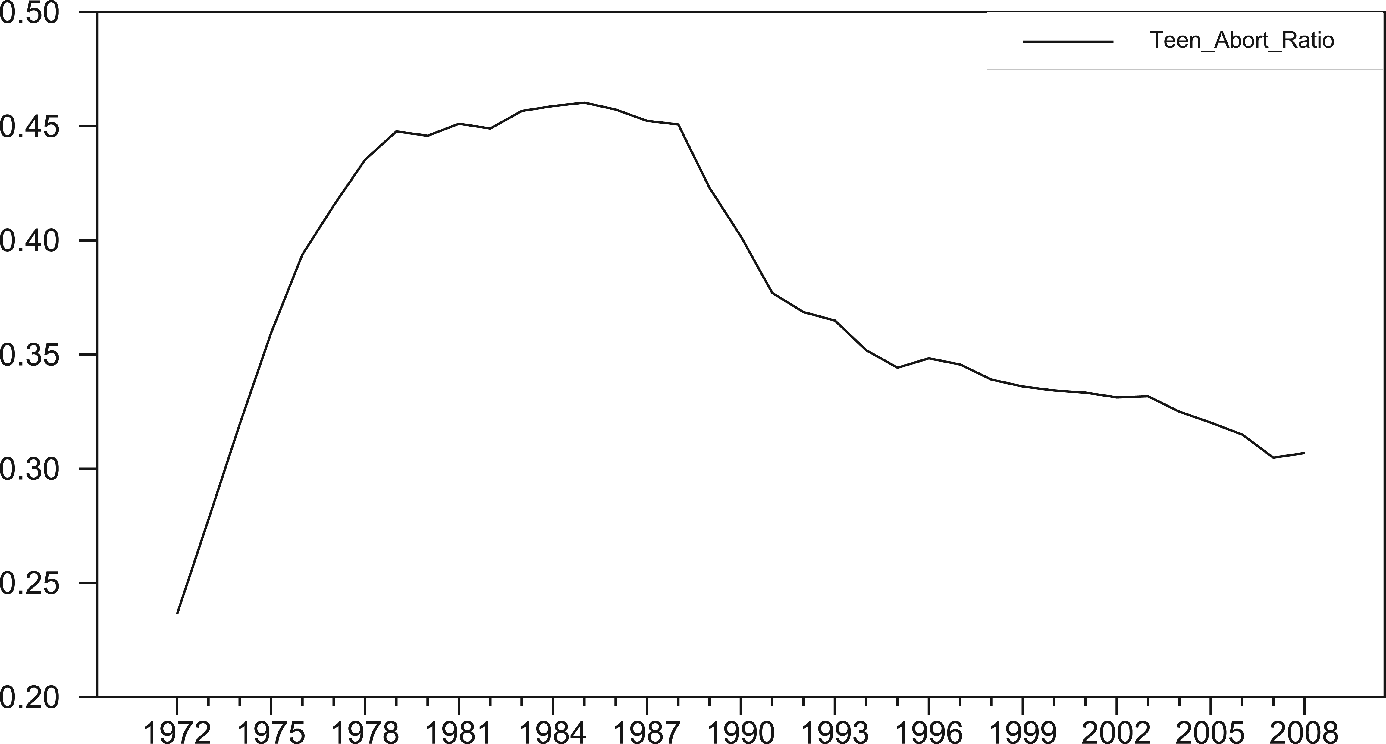
Figure 4 shows U.S. teenage abortion ratios for 1972-2008. Although abortion ratios by state are not available for the 1970s, U.S. ratios are roughly the same from 1976 to 1988. Given that the relative magnitudes of the weighted abortion ratios between the top and bottom 14 states are stable for the 21 years 1988-2008, even as teenage weighted abortion ratios dropped substantially, it is reasonable to assume that relative teenage abortion ratios did not change appreciably across states projecting back to the 1970s. With this assumption, states where crime is most responsive to total abortion rates (Table 3) are the same states with the highest teenage weighted abortion ratios and the opposite for the bottom 14 states. Although somewhat ad hoc, this approach overcomes, to the extent possible, the lack of state-level teenage abortion data for the 1970s.

Figure 4.

U.S. teenage (15-19) abortion ratio.

As a further test, states ranked by average significance in the last column of Table 3 are reassigned ranks of 1 to 50; Colorado being 50, Mississippi being 1. Teenage weighted abortion ratios are also ranked 1 to 50, 50 again being the highest. Regressing all 50 states’ significance ranks on a constant and their teenage abortion ranks, the coefficient (standard error) on teenage abortion is .529 (.122), thus, a positive and significant relationship. Removing the five outliers in the lower-right corner of Figure 3 (North Carolina, Delaware, Nevada, Maryland, and Hawaii), the result is .761 (.117), and the hypothesis that the coefficient is 1.0 is marginally rejected with a p-value of .047.⁸ Using only the top and bottom 14 states, the result is .975 (.143), failing to reject that the coefficient is 1.0 with a p-value of .861. Thus, excluding the five outliers or considering only the top and bottom 14 states, there is a near one-to-one correspondence across states between the ranked significance of total abortions in explaining crime and ranked teenage abortion ratios.

As further evidence, Figure 5 shows the more familiar abortion rate for each state versus the same ranked significance values in Figure 3. The top and bottom 14 states are again nearly polarized. Using abortion rates allows for another useful comparison. In Figure 6, average significance ranks are charted against the difference between teenage (15-19) abortion rates and adult (20-44) abortion rates.⁹ The top and bottom 14 states are again polarized, showing that the top 14 states are much more heavily engaged in teenage (15-19) abortions than adult (20-44) abortions compared with other states, and the opposite for the bottom 14 states.

Figure 5.

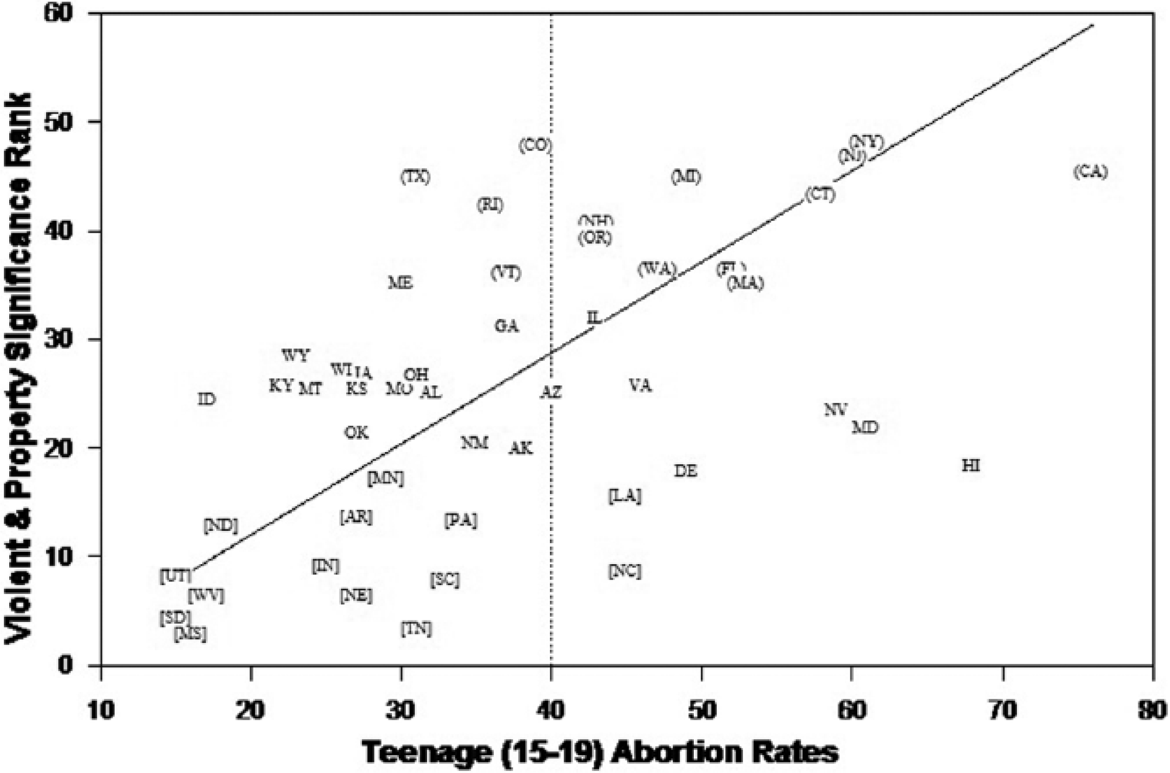
Teenage abortion rates and ranked significance of abortion modeling crime.

Figure 6.

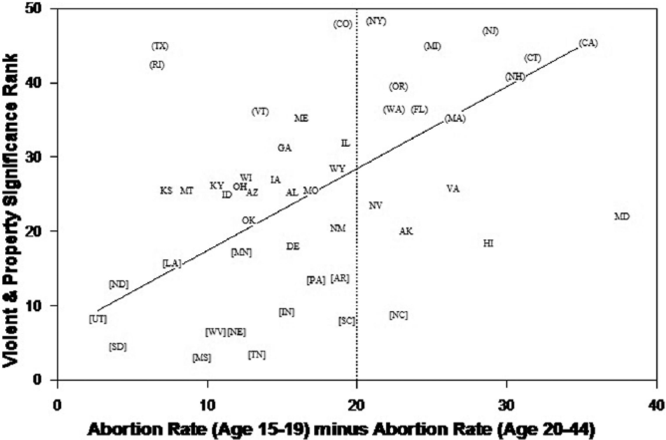
Difference in teenage and adult abortion rates and ranked abortion significance.

Recalling Tennessee and Michigan in Figure 1, long-differenced violent crime effective abortion rates are 135 for Tennessee and 172.94 for Michigan, a 28.1% difference. For property crime (Figure 2), the difference is 28.7%. In contrast, Figure 3 shows a 57.1% difference in teenage weighted abortion ratios, Figure 5 a 64.5% difference in teenage abortion rates, and Figure 6 an 88.5% difference in teenage abortion rates minus adult abortion rates. Thus, the gaps in long-differenced crime for Tennessee and Michigan are consistent with differences in teenage abortions in the states. Similar comparisons apply to many states with midrange values of long-differenced effective abortion rates in Figures 1 and 2.

Modeling Arrests and the 2008 Data Set

This section analyzes DL’s (Table VI, p. 400) panel-data models of arrests per capita with the 2001 and 2004 data sets, repeats the analyses using DL’s (2008) data set, then estimates DL’s (Table VII, p. 413) state–year–age models of arrests using the 2008 data set. Like the models of crime, in each case, the states that drive the significant relationships between crime and abortion are states with high concentrations of teenage abortions. Because the procedures are the same as those described above, the evidence is reported in summary fashion.

Table 5 shows summary results for DL’s (Table VI, p.409) panel-data models of arrests using the 2001 and 2004 data sets, comparable with Table 2, but without reporting the coefficients for the eight control variables still included in the models. The first two regressions in the first panel of Table 5 replicate DL’s results for under age 25 arrests. The second two regressions are similar, but use the 2004 data set. The second panel again includes differenced models that exclude DC and drop population weighting. The coefficients in the second panel are not all significant at the .05 level, but are significant at similar levels as DL’s original coefficients.

Table 5.

DL (2001) U.S. National Panel-Data Models of Violent and Property Arrests.

	2001 data set		2004 data set
	(Δ)ln(Violent crime arrests per capita)_t	(Δ)ln(Property crime arrests per capita)_t	(Δ)ln(Violent crime arrests per capita)_t	(Δ)ln(Property crime arrests per capita)_t
DL original GLS specification; 50 states plus DC, population weighted
Effective Abortion Rate (×100)_t	−.044 (−1.49)	−.054 (−2.35*)	−.049 (−1.42)	−.064 (−2.57*)
R ²	.985	.982	.982	.975
OLS in first differences, 50 states, unweighted
ΔEffective Abortion Rate (×100)_t	−.143 (−1.78)	−.101 (−2.26*)	−.153 (−1.68)	−.133 (−2.51*)
R ²	.111	.089	.115	.090
DL original GLS specification; 37 states, population weighted^a
Effective Abortion Rate (×100)_t	−.091 (−.84)	−.062 (−1.06)	−.167 (−1.45)	−.093 (−1.81)
R ²	.965	.972	.879	.977
OLS in first differences, 37 states, unweighted
ΔEffective Abortion Rate (×100)_t	−.139 (−1.01)	−.099 (−1.52)	−.078 (−.82)	−.108 (−1.84)
R ²	.113	.107	.144	.095

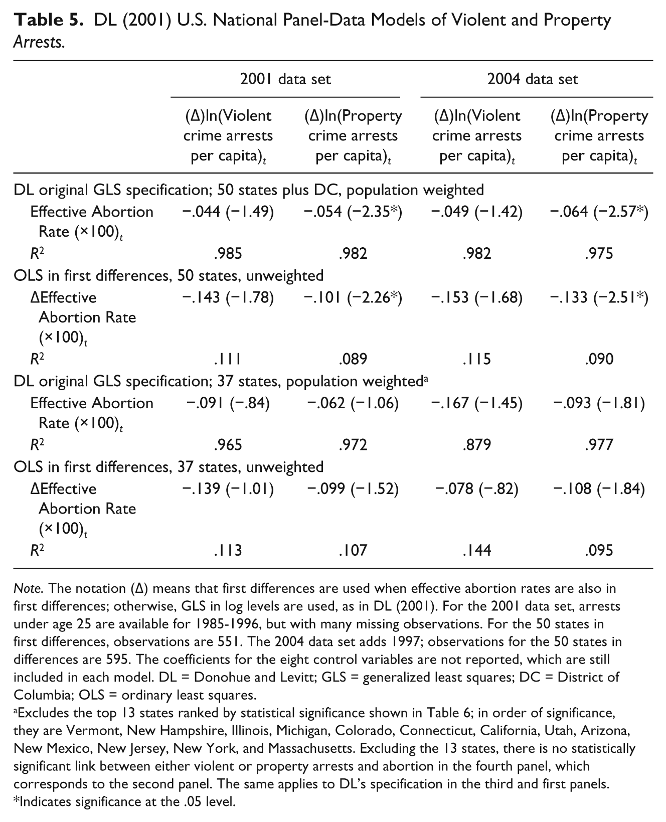
Note. The notation (Δ) means that first differences are used when effective abortion rates are also in first differences; otherwise, GLS in log levels are used, as in DL (2001). For the 2001 data set, arrests under age 25 are available for 1985-1996, but with many missing observations. For the 50 states in first differences, observations are 551. The 2004 data set adds 1997; observations for the 50 states in differences are 595. The coefficients for the eight control variables are not reported, which are still included in each model. DL = Donohue and Levitt; GLS = generalized least squares; DC = District of Columbia; OLS = ordinary least squares.

Excludes the top 13 states ranked by statistical significance shown in Table 6; in order of significance, they are Vermont, New Hampshire, Illinois, Michigan, Colorado, Connecticut, California, Utah, Arizona, New Mexico, New Jersey, New York, and Massachusetts. Excluding the 13 states, there is no statistically significant link between either violent or property arrests and abortion in the fourth panel, which corresponds to the second panel. The same applies to DL’s specification in the third and first panels.

Indicates significance at the .05 level.

After rank ordering the states for each of the 2001 and 2004 data sets and both violent and property arrests, the average significant ranks are again computed. For ease of comparison, the states are re-ranked 1 to 50 based on their average significance ranks. In this case, eliminating only 13 states yields insignificant abortion coefficients for all four models in the bottom panel of Table 5. The states are Vermont, New Hampshire, Illinois, Michigan, Colorado, Connecticut, California, Utah, Arizona, New Mexico, New Jersey, New York, and Massachusetts. The last 13 states are South Carolina, Louisiana, Iowa, Arkansas, Alabama, Kansas, Nebraska, Tennessee, Montana, Wyoming, South Dakota, North Carolina, and Kentucky.

Although the number of excluded states required to yield insignificant results is not the same for crime and arrests (14 vs. 13), hypergeometric distributions are still used to assess the relatedness of the lists of states. In this case, the number of members is again 50, the number of successes (top-ranked states for crime) is 14, and the “random” sample without replacement is 13 (top-ranked states for arrests). The calculated probability is still for the number of matching states in the sample of 13 (ranks ≥ 38) compared with the 14 states for crime (ranks ≥ 37). (Hypergeometric distributions are often described in terms of red and black balls. Here, there are 14 red balls and 36 black balls. A sample without replacement of 13 is taken. The probability calculated still applies to the number of matches, that is, red balls.)

The first two columns of Table 6 show the 2001/2004 results for crime and arrests ranked 1 to 50. For the top 14 crime states and 13 arrests states, there are nine matches; the probability of nine or more matches being .00035. Comparing the bottom 14 states for crime (ranks 1-14) and arrests (ranks 1-13), there are seven matches (probability .02238). As with crime, the states that drive the link between arrests and abortions have high teenage weighted abortion ratios, and the opposite for the bottom 13 states.

Table 6.

State Significance Ranks Using Effective Abortion Rates to Model Crime and Arrests.

	Data sets
	2001/2004		2008
	Significance rank modeling		Significance rank modeling
State	Crime	Arrests	Crime	Arrests
Colorado	50	46	49	45
New York	49	39	50	41
New Jersey	48	40	48	44
California	47	44	45	42
Michigan	46	47	47	48
Texas	45	35	44	36
Connecticut	44	45	45	39
Rhode Island	43	36	43	40
Oregon	42	22	42	31
New Hampshire	41	49	41	47
Washington	40	28	38	26
Vermont	39	50	36	50
Florida	38	19	40	20
Massachusetts	37	38	37	35
Maine	36	21	39	17
Illinois	35	48	35	49
Georgia	34	16	34	34
Wyoming	33	10	33	10
Wisconsin	32	15	28	9
Ohio	31	29	26	38
Kansas	30	6	16	5
Kentucky	29	13	22	12
Missouri	28	37	19	37
Virginia	27	23	25	22
Alabama	26	5	27	8
Iowa	25	3	21	1
Montana	24	9	32	14
Arizona	23	42	29	46
Idaho	22	34	31	28
Nevada	21	26	30	29
Maryland	20	30	18	33
Oklahoma	19	20	17	24
New Mexico	18	41	23	30
Alaska	17	27	24	19
Hawaii	16	31	14	32
Delaware	15	33	13	27
Minnesota	14	17	15	13
Louisiana	13	2	20	2
Arkansas	12	4	12	6
Pennsylvania	11	32	9	25
North Dakota	10	18	11	23
Indiana	9	24	6	18
North Carolina	8	12	7	16
Utah	7	43	10	43
South Carolina	6	1	5	3
Nebraska	5	7	3	4
West Virginia	4	25	2	21
South Dakota	3	11	8	7
Tennessee	2	8	4	11
Mississippi	1	14	1	15

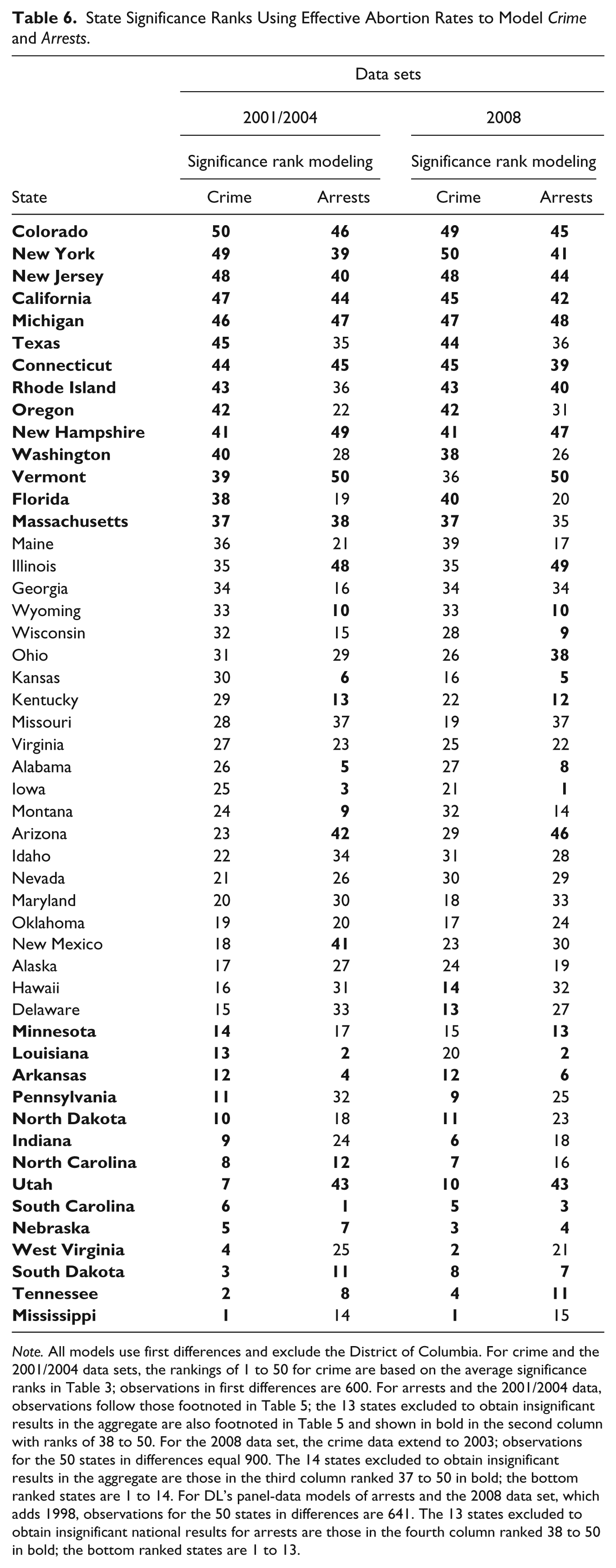
Note. All models use first differences and exclude the District of Columbia. For crime and the 2001/2004 data sets, the rankings of 1 to 50 for crime are based on the average significance ranks in Table 3; observations in first differences are 600. For arrests and the 2001/2004 data, observations follow those footnoted in Table 5; the 13 states excluded to obtain insignificant results in the aggregate are also footnoted in Table 5 and shown in bold in the second column with ranks of 38 to 50. For the 2008 data set, the crime data extend to 2003; observations for the 50 states in differences equal 900. The 14 states excluded to obtain insignificant results in the aggregate are those in the third column ranked 37 to 50 in bold; the bottom ranked states are 1 to 14. For DL’s panel-data models of arrests and the 2008 data set, which adds 1998, observations for the 50 states in differences are 641. The 13 states excluded to obtain insignificant national results for arrests are those in the fourth column ranked 38 to 50 in bold; the bottom ranked states are 1 to 13.

Several states in Figure 3 with high teenage weighted abortion ratios move upward in significance rank. For arrests, Arizona and New Mexico move up to the top 13. Maryland, Hawaii, and Delaware also move upward. Georgia, Oregon, and Florida move downward. Thus, the highest ranked states are still those with high weighted teenage abortion ratios, but reordered to a small degree. The third and fourth columns of Table 6 show the results of modeling crime and arrests using the 2008 data set. Removing the top 14 states again results in insignificant national abortion coefficients for crime and 13 states again for arrests.

For crime alone, Table 6 shows that 13 of the top 14 states are the same in the 2001/2004 and 2008 data sets and 12 of the bottom 14. For arrests, across 2001/2004 and 2008 data sets, 11 of the top 13 states are the same and 11 of the bottom 13. For 2008 only, comparing crime ranks 37 to 50 and arrests ranks 38 to 50, there are nine matches, but for the bottom 14 crime states and bottom 13 arrests states, there are only five matches; the probability of five or more being .26374, the weakest comparison observed here, although not surprising given the widespread insignificance of abortion coefficients in Table 5.

Having compared many lists of states, it is useful to use an overall indicator that directly compares the states that drive the significant relationships between crime and abortion and the states having high teenage weighted abortion ratios. Across the lists of states in Table 6, there are 54 states that drive the relationships between crime/arrests and abortion; 14 in the first and third columns and 13 in the second and fourth columns. Of the 54 states, 47 (87.0%) have teenage weighted abortion ratios greater than .40, the midpoint of the ratios in Figures 3 and 5. Of the bottom-ranked 54 states, 50 (92.6%) have teenage weighted abortion ratios less than .40. Seven states appear in the top 14 states in all four lists: Colorado, New York, New Jersey, California, Michigan, Connecticut, and New Hampshire. Vermont, Massachusetts, and Rhode Island are close behind, with three out of four ranks ≥ 37 and the other rank being 35 or 36.

Turning to long differences, the 2008 data set extends the crime data to 2003. The t statistic for long-differenced violent crime effective abortion rates is −4.75 with all 50 states. Excluding the top 14 states and Vermont (rank 36), the t statistic is −1.89. For property crime, the t statistic for abortion declines from −4.39 to −1.27 by eliminating the top 14 states.

DL’s (Table VII, p. 413) state–year–age models of arrests and 2008 data set have received much attention, mainly because the model includes actual abortion rates, rather than effective abortion rates, plus data for arrests by state by single year of age. For purposes here, there is no obvious model among the multiple specifications in Foote and Goetz (2008) and DL (2008) to identify the states that drive a significant link between arrests and abortion. However, the intent here is to show that under any of DL’s specifications and any of the three data sets, if a significant link occurs between crime and abortion, it is due to a handful of states with high teenage abortion ratios. Therefore, the specification and data set used to address DL’s Table VII results are the ones that favor DL most, that is, DL’s original model and 2008 data set.

As expected, the 2008 data set yields larger coefficients than DL’s original Table VII, Columns 3 and 7. For violent crime, the original abortion coefficient (t statistic) of −.028 (−6.48) becomes −.035 (−5.46). For property crime, −.025 (−8.78) becomes −.036 (−7.24). In this case, excluding only 12 states results in insignificant abortion coefficients; they are Illinois, Michigan, Vermont, Delaware, New York, New Jersey, Iowa, New Mexico, Massachusetts, Connecticut, Colorado, and Kentucky. Of the 12, nine have teenage weighted abortion ratios of .40 or higher, plus New Mexico at .39. The bottom 12 states are Nevada, South Carolina, Georgia, Oregon, Arkansas, Washington, South Dakota, Minnesota, Wisconsin, Alabama, Wyoming, and Virginia. Seven of the 12 states have teenage weighted abortion ratios less than .40 plus Georgia at .41.

Conclusions and Future Research

This study shows that, if there is a significant link between crime and abortion, it is due to varying concentrations of teenage abortions across states, not unwantedness. All evidence is mutually supportive. The state-by-state crime and arrests panel-data results plus Rasanen et al.’s (1999) odds ratios imply the observed Allan Guttmacher Institute state-by-state teenage weighted abortion ratios. The state-by-state panel-data results plus the teenage abortion data imply Rasanen et al.’s odds ratios. And Rasanen et al.’s results plus the teenage abortion data imply the panel-data results. All agree with Torres and Forrest’s (1988) report on the reasons women had abortions by age group. Moreover, the combined evidence in Rasanen et al., Morash and Rucker (1989), Torres and Forrest (1988), Hay and Evans (2006), and Hunt (2006) effectively rejects DL’s “unwantedness leads to high crime” hypothesis, while verifying the major role of teenage motherhood.

A summary of the results is as follows: (a) DL’s conclusions about abortion apply much more to teenagers than adult women, who now account for more than 80% of U.S. abortions, (b) the odds of a child from an unwanted pregnancy becoming a criminal decline rapidly as the mother’s age and education increase, (c) half of all abortions have virtually no effect on crime, (d) unwantedness affects crime no more than mothers who smoke and is insignificant based on U.S. data, and (e) with teenage abortion rates declining from 43.5 in 1988 to 22.5 in 2001, it is likely that all of DL’s panel-data models were outdated when published. In short, three million teenagers had abortions in the 1970s and crime fell in the 1990s, the second possibly related to the first. If the two are related, it is due to three million fewer teenage mothers, not less unwantedness.

As already mentioned, for future research, the relationship between crime and abortion may be clarified by repeating earlier studies, but including only states with distinctly high and low teenage abortion concentrations. This effort may help settle the long-disputed issue of crime and abortion. Research aimed at reducing teenage pregnancy should also be a priority, supported by additional research on the sociological and psychological behavior of teenagers.

Last, this study is not meant to encourage teenage abortion. Fortunately, with teenage pregnancies declining faster than teenage abortions, the U.S. teenage birthrate was 34.3 births per 1,000 teenage women in 2010, a 41.1% decline from 1990 and a 49.8% decline from 1970 (Centers for Disease Control [CDC]). The most recent decline in teenage births is linked almost exclusively to improved contraceptive use (CDC National Survey of Family Growth).

Footnotes

Acknowledgements

The author thanks Thomas Marvell and Paul Zimmerman for many helpful comments on an earlier version of the article. Thanks also go to Jon Pinder for recommending hypergeometric distributions as a means of assessing similarities in lists of states. Finally, John Donohue, Steven Levitt, Christopher Foote, and Christopher Goetz provided their data sets, which are publicly available at http://islandia.law.yale.edu/donohue/pubsdata.htm and .

Declaration of Conflicting Interests

The author(s) declared no potential conflicts of interest with respect to the research, authorship, and/or publication of this article.

Funding

The author(s) disclosed receipt of the following financial support for the research, authorship, and/or publication of this article: The research grants program of the Wake Forest University School of Business supported this research.

Notes

Author Biography

Gary L. Shoesmith is a professor of economics at Wake Forest University’s School of Business. His research interests include crime modeling and forecasting, time-series analysis, national and regional forecasting, and financial market microstructure. He has publications in International Journal of Forecasting, Journal of Financial and Quantitative Analysis, Journal of Regional Science, Journal of Banking and Finance, and others. His education includes a PhD from Southern Methodist University, an MS in economics from Iowa State University, and a BS in mathematics and economics from Pittsburg State University. Prior to academia, he was the chemicals division economist at Phillips Petroleum Company and, before that, an economic consultant with Data Resources, Inc. (now Information Handling Services [IHS] Global Insight).

References

Anderson

Wells

(2008). Numerical analysis in least squares regression with an application to the abortion-crime debate. Journal of Empirical Legal Studies, 5, 647-681.

Anderson

Wells

(2010). A Bayesian hierarchical regression approach to clustered and longitudinal data in empirical legal studies. Journal of Empirical Legal Studies, 7, 634-663.

Baumer

E. P.

Wolff

K. T.

(2014). Evaluating contemporary crime drop(s) in America, New York City, and many other places. Justice Quarterly, 31, 5-38.

Bhargava

Franzini

Narendranathan

(1982). Serial correlation and the fixed effects model. Review of Economic Studies, 49, 533-549.

Chamlin

M. B.

Myer

A. J.

Sanders

B. A.

Cochran

J. K.

(2008). Abortion as crime control: A cautionary tale. Criminal Justice Policy Review, 19, 135-152.

Comanor

W. S.

Phillips

(1999). The impact of income and family structure on delinquency. Unpublished Manuscript, University of California, Santa Barbara.

DeFina

R. H.

Arvanites

T. M.

(2002). The weak effect of imprisonment on crime: 1971-1998. Social Science Quarterly, 83, 635-653.

Donohue

J. J.

Levitt

S. D.

(2001). The impact of legalized abortion on crime. Quarterly Journal of Economics, 116, 379-420.

Donohue

J. J.

Levitt

S. D.

(2004). Further evidence that legalized abortion lowered crime: A reply to Joyce. Journal of Human Resources, 39, 29-49.

10.

Donohue

J. J.

Levitt

S. D.

(2008). Measurement error, legalized abortion, and the decline in crime: A response to Foote and Goetz. Quarterly Journal of Economics, 123, 425-440.

11.

Evans-Chase

Kim

Zhou

(2013). Risk-taking and self-regulation: A systematic review of the analysis of delinquency outcomes in the juvenile justice intervention literature 1996-2009. Criminal Justice and Behavior, 40, 608-628.

12.

Foote

C. L.

Goetz

C. F.

(2008). The impact of legalized abortion on crime: Comment. Quarterly Journal of Economics, 123, 407-423.

13.

Francois

Magni-Berton

Weill

(2014). Abortion and crime: Cross-country evidence from Europe. International Review of Law and Economics, 40, 24-35.

14.

Hay

Evans

M. M.

(2006). Has Roe v. Wade reduced U.S. crime rates? Journal of Research in Crime & Delinquency, 43, 36-66.

15.

Henshaw

S. K.

(1993). Teenage abortion, birth and pregnancy statistics by state, 1988. Family Planning Perspectives, 25, 122-126.

16.

Henshaw

S. K.

(1997). Teenage abortion and pregnancy statistics by state, 1992. Family Planning Perspectives, 29, 115-122.

17.

Henshaw

S. K.

Kost

(2008). Trends in the characteristics of women obtaining abortions, 1974 to 2004. New York, NY: Allan Guttmacher Institute.

18.

Henshaw

S. K.

Van Vort

(1990). Abortion services in the United States, 1987 and 1988. Family Planning Perspectives, 22, 102-108.

19.

Hunt

(2006). Do teen births keep American crime high? Journal of Law and Economics, 49, 533-566.

20.

Jones

R. K.

Finer

L. B.

Singh

(2010). Characteristics of U.S. abortion patients, 2008. New York, NY: Allan Guttmacher Institute.

21.

Jones

R. K.

Kooistra

(2011). Abortion incidence and access to services in the United States, 2008. Perspectives on Sexual and Reproductive Health, 43, 41-50.

22.

Joyce

(2004). Did legalized abortion lower crime? Journal of Human Resources, 39, 1-28.

23.

Joyce

(2009). A simple test of abortion and crime. Review of Economics and Statistics, 91, 112-123.

24.

Kost

Henshaw

(2012). U.S. teenage pregnancies, births and abortions, 2008: National trends by age, race and ethnicity. New York, NY: Allan Guttmacher Institute.

25.

Levitt

S. D.

(2004). Understanding why crime fell in the 1990s: Four factors that explain the decline and six that do not. Journal of Economic Perspectives, 18, 163-190.

26.

Levitt

S. D.

Dubner

S. J.

(2005). Freakonomics: A rogue economist explores the hidden side of everything. New York, NY: HarperCollins.

27.

Lott

J. R.

Whitley

(2007). Abortion and crime: Unwanted children and out-of-wedlock births. Economic Inquiry, 45, 304-324.

28.

Manlove

Wildsmith

Welti

Scott

M. E.

Ikramullah

(2012). Relationship characteristics and the relationship context of nonmarital first births among young adult women. Social Science Quarterly, 93, 506-520.

29.

Marvell

T. B.

(2010). Prison population and crime. In Benson

Zimmerman

(Eds.), Handbook on the economics of crime (pp. 145-183). Northampton, MA: Edward Elgar.

30.

Marvell

T. B.

Moody

C. E.

(1998). The impact of out-of-state prison population on state homicide rates: Displacement and free-rider effects. Criminology, 36, 513-535.

31.

Moody

C. E.

Marvell

T. B.

(2010). On the choice of control variables in the crime equation. Oxford Bulletin of Economics and Statistics, 72, 696-715.

32.

Morash

Rucker

(1989). An exploratory study of the connection of mother’s age at childbearing to her children’s delinquency in four data sets. Crime & Delinquency, 35, 45-93.

33.

Rasanen

Helina

Isohanni

Hodgins

Jarvelin

Tiihonen

(1999). Maternal smoking during pregnancy and risk of criminal behavior among adult male offspring in the Northern Finland 1966 Birth Cohort. American Journal of Psychiatry, 156, 857-862.

34.

Scott

E. S.

Rappucci

N. D.

Woolard

J. L.

(1995). Evaluating adolescent decision making in legal contexts. Law and Human Behavior, 19, 221-244.

35.

Shattuck

Kreider

(2013). Social and economic characteristics of currently unmarried women with a recent birth: 2011. Retrieved from https://www.census.gov/prod/2013pubs/acs-21.pdf

36.

Thomas

(2012). Three strategies to prevent unintended pregnancies. Journal of Policy Analysis and Management, 31, 280-311.

37.

Torres

Forrest

(1988). Why do women have abortions? Family Planning Perspectives, 20, 169-176.

Crime,Teenage Abortion,and Unwantedness

Abstract

Keywords

The Odds of Becoming a Criminal

National (Aggregate) Panel-Data Results for Crime

State-by-State (Disaggregate) Panel-Data Results for Crime

DL’s Long Differences

State-by-State, Teenage Abortion and Crime

Modeling Arrests and the 2008 Data Set

Conclusions and Future Research

Footnotes

Acknowledgements

Declaration of Conflicting Interests

Funding

Notes

Author Biography

References