Sage Journals: Discover world-class research

Abstract

Suppose a random vector $(U_{1}, \dots, U_{d})$ with values in the unit cube has a joint survival function: $C^{*} (u_{1}, \dots, u_{d}) = ℙ (U_{1} > u_{1}, \dots, U_{d} > u_{d}),$

given by an Archimedean copula $C (u_{1}, \dots, u_{d}) = φ^{- 1} (φ (u_{1}) + \dots + φ (u_{d})),$

with generator $φ : [0, 1]\to[0, \infty)$ , a smooth decreasing convex function such that $φ (1) = 0$ . In this article, we provide a formula for the distribution of $Z = C^{*} (U_{1}, \dots, U_{d}) = ℙ (U_{1}^{'} > U_{1}, \dots, U_{d}^{'} > U_{d} ∣ U_{1}, \dots, U_{d}),$

where $(U_{1}^{'}, \dots, U_{d}^{'})$ is an independent copy of $(U_{1}, \dots, U_{d})$ and a method to simulate values from the distribution of Z in the bivariate case, that is, when d = 2. The case d > 2 does not seem to be tractable. As an application, we show how our result can be used to compute the limiting covariance of the empirical Kendall process corresponding to $C^{*} (U_{1}, U_{2})$ .

AMS Subject Classification: 62H05

Keywords

Archimedean copula Kendall distribution Kendall process

1. Introduction

It is well known that if X is a continuous random variable with cumulative distribution function F(.), then both F(X) and 1 - F(X) are uniformly distributed over [0, 1]. This result is known as the probability integral transformation (PIT). Extension of the PIT to two or more dimensions is not at all straightforward, primarily because of the lack of linear order in higher dimensions. Note that in two dimensions, the problem would be to find the distribution of $F (X_{1}, X_{2})$ or $\bar{F} (X_{1}, X_{2})$ , where $(X_{1}, X_{2})$ are random variables with joint continuous distribution function F(.,.) and $\bar{F} (x_{1}, x_{2}) = P [X_{1} > x_{1}, X_{2} > x_{2}]$ is the joint survival function. While partial answers are known for $F (X_{1}, X_{2})$ , nothing is known for $\bar{F} (X_{1}, X_{2})$ . The goal of this article is to provide a partial solution to the latter problem.

This type of results are important because of their potential use in goodness-of-fit and estimation procedures.

We obtain our results in the framework of copulas. A copula is a tool for modelling a joint distribution in terms of its margins. More precisely, a d-variate copula $C (u_{1}, \dots, u_{d})$ is the joint cumulative distribution function of random variables $(U_{1}, \dots, U_{d})$ . where $0 \leq U_{j} \leq 1, 1 \leq j \leq d, d \geq 2$ . In particular, a bivariate copula $C (u_{1}, u_{2})$ is a bivariate distribution $[0, 1]\times[0, 1]\to[0, 1]$ with the properties:

(1) $C (u_{1}, 0) = C (0, u_{2}) = 0,$

(2) $C (u, 1) = C (1, u) = u$ ,

(3) and $C (u_{2}, v_{2}) + C (u_{1}, v_{1}) \geq C (u_{2}, v_{1}) + C (u_{1}, v_{2})$ for $0 \leq u_{1} \leq u_{2} \leq 1$ and $0 \leq v_{1} \leq v_{2} \leq 1$ .

Consider a pair $(X_{1}, X_{2})$ of real valued random variables with joint distribution $F (x_{1}, x_{2}) = ℙ (X_{1} \leq$ $x_{1}, X_{2} \leq x_{2})$ and marginal distribution functions $F_{1} (x_{1}) = ℙ (X_{1} \leq x_{1})$ and $F_{2} (x_{2}) = ℙ (X_{2} \leq x_{2})$ .

By Sklar’s theorem,^[1] the joint distribution $F$ , if continuous, can be expressed via a unique copula $C$ :

\begin{matrix} F (x_{1}, x_{2}) = ℙ (X_{1} \leq x_{1}, X_{2} \leq x_{2}) = C (F_{1} (x_{1}), F_{2} (x_{2})) . \end{matrix}

(1.1)

When considered as random variables, the distribution function $F (X_{1}, X_{2})$ and the copula $C (U_{1}, U_{2})$ (where $U_{1}$ and $U_{2}$ are two uniform random variables with joint distribution C) have the same distribution function, which is known as the 'Kendall distribution function' of the pair $(X_{1}, X_{2})$ :

\begin{matrix} K (z) : = ℙ (C (U_{1}, U_{2}) \leq z), for z \in [0, 1] . \end{matrix}

(1.2)

Chakak and Ezzerg^[2] provided a general formula for the distribution of a copula $C (U_{1}, U_{2})$ :

\begin{matrix} K (z) = z + \int_{z}^{1} (\int_{0}^{ψ (z, u_{1})} c (u_{1}, u_{2}) d u_{2}) d u_{1}, 0 < z \leq 1, \end{matrix}

(1.3)

where $c (x_{1}, x_{2}) = \frac{\partial^{2}}{\partial x \partial y} C (x_{1}, x_{2})$ is the joint density of a pair $(X_{1}, X_{2}) \sim C$ and

ψ (z, u_{1}) = inf \{u_{2} : C (z, u_{2}) \geq z\}

for $0 < z \leq u_{1} \leq 1$ is the quantile function of the copula C. However, for numerical applications, the quantile function $ψ$ is not always available.

A particular class of copulas is the 'Archimedean' family. They are copulas such that $C (u_{1}, u_{2}) = φ^{- 1} (φ (u_{1}) + φ (u_{2}))$ , where $φ : [0, 1]\to[0, \infty)$ is a continuous, decreasing convex function such that $φ (1) = 0$ . Information about the bivariate distribution function is contained in the univariate function $φ$ , called 'the generator' of the copula.

Genest and Rivest^[3] established that the Kendall distribution function of an Archimedean copula $C (u_{1}, u_{2}) = φ^{- 1} (φ (u_{1}) + φ (u_{2}))$ is

\begin{matrix} K (z) = z - \frac{φ (z)}{φ^{'} (z)} for z \in (0, 1) . \end{matrix}

(1.4)

\begin{matrix} φ (z) = φ (z_{0}) exp [\int_{z_{0}}^{z} \frac{d u_{2}}{v - K (u_{2})}] for an arbitrary constant 0 < z_{0} < 1, \end{matrix}

(1.5)

K is important for identifying $φ$ , hence C (in the case of Archimedean copulas).

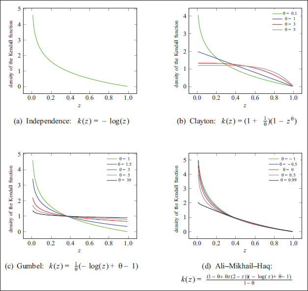
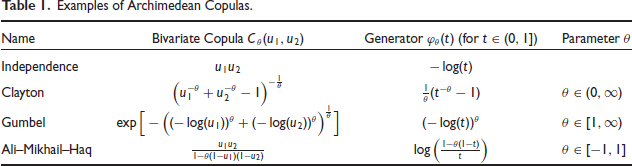
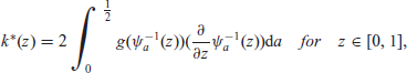
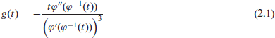
Figures 1a-d display the density $k (z)$ of the Kendall function for some Archimedean copulas.

Figure 1.

Density $k (z), z \in (0, I)$ , of the Kendall Distribution for Some Archimedean Copulas.

The goal of this work is to obtain the density function of the 'joint survival function' of two standard uniform random variables $U_{1}, U_{2}$ with (joint) distribution given by an Archimedean copula C, that is, the density of

\begin{matrix} C^{*} (U_{1}, U_{2}) = 1 - U_{1} - U_{2} + C (U_{1}, U_{2}) . \end{matrix}

(1.6)

Note that

\begin{matrix} C^{*} (u_{1}, u_{2}) = P (U_{1} > u_{1}, U_{2} > u_{2}) . \end{matrix}

(1.7)

Note that Genest and Rivest’s^[3] result (Equation (1.4)) is an analogue of the PIT for $C (F_{1} (X_{1}), \dots, F_{d} (X_{d}))$ in the case of an Archimedean copula. We complement their result for

C^{*} (F_{1} (X_{1}), F_{2} (X_{2}))

in the bivariate case.

We obtain the distribution by observing that $C^{*} (U_{1}, U_{2})$ has the same distribution as $1 - φ^{- 1} (W T) -$ $φ^{- 1} ((1 - W) T) + φ^{- 1} (T)$ where W and T are independent, W has a uniform distribution on (0, 1) and T is from some density g (.) (see Equation (2.1), Theorem 2.1). T is linked to the copula by the fact that $C (U_{1}, U_{2})$ has the same distribution as $φ^{- 1} (T)$ (see Corollary 2.1).

As for applications, our result complements Equation (1.4) and may be used for copula-based estimation and goodness-of-fit procedures, as in Genest et al.^[4]. We illustrate this in Section 3.2 using samples simulated from the Clayton copula. Another important application is given in our Theorem 2.2, where, following Barbe et al.,^[5] we derive the weak convergence of the empirical Kendall process of $C_{n}^{*} (U_{1 i}, U_{2 i}), 1 \leq i \leq n$ . Here $C_{n}^{*} (.,)$ . is the empirical version of $C^{*} (.,)$ Barbe et al.^[5]. Clearly, the covariance of the limiting Gaussian process in this theorem would be hard to compute without using our result (Theorem 2.1).

In Section 2, we present our result for the bi-variate case, that is, for $C^{*} (U_{1}, U_{2})$ , and the weak convergence result, in addition to examples from the models mentioned in Table 1. In Section 3.1, plots of densities of $C^{*}$ from these models are presented. In Section 3.2, we present a comparison between the density computed using our result and the density estimated from simulated $C^{*} (U_{1}, U_{2})$ values. Here we also present illustrations of distance-statistics based on the empirical process of simulated $C^{*} (U_{1}, U_{2})$ values, which can be minimized to estimate the copula-parameter.

Table 1.

Examples of Archimedean Copulas.

Name	Bivariate Copula $C_{θ} (u_{1}, u_{2})$	Generator $φ_{θ} (t)$ (for $t \in (0, I])$	Parameter $θ$
Independence	$u_{1} u_{2}$	$- log (t)$
Clayton	${(u_{1}^{- θ} + u_{2}^{- θ} - 1)}^{- \frac{1}{θ}}$	$\frac{1}{θ} (t^{- θ} - I)$	$θ \in (0, \infty)$
Gumbel	$exp [- {({(- log (u_{1}))}^{θ} + {(- log (u_{2}))}^{θ})}^{\frac{1}{θ}}]$	${(- log (t))}^{θ}$	$θ \in [1, \infty)$
Ali-Mikhail-Haq	$\frac{u_{1} u_{2}}{1 - θ (1 - u_{1}) (1 - u_{2})}$	$log (\frac{1 - θ (1 - t)}{t})$	$θ \in [- 1, 1]$

2. Main Result

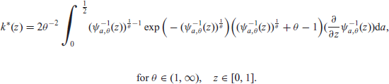
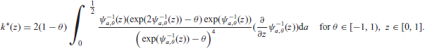
Theorem 2.1. Let U and V be two uniform random variables with joint distribution the Archimedean copula $C (u_{1}, u_{2}) = φ^{- 1} (φ (u_{1}) + φ (u_{2}))$ . The density of the survival distribution $C^{*} (U_{1}, U_{2})$ is

k^{*} (z) = 2 \int_{0}^{\frac{1}{2}} g (ψ_{a}^{- 1} (z)) (\frac{\partial}{\partial z} ψ_{a}^{- 1} (z)) d a for z \in [0, 1],

where

\begin{matrix} g (t) = - \frac{t φ^{″} (φ^{- 1} (t))}{{(φ^{'} (φ^{- 1} (t)))}^{3}} \end{matrix}

(2.1)

and

\begin{matrix} ψ_{a} (b) = ℙ (\frac{φ (U_{1})}{a} \leq b, \frac{φ (U_{2})}{1 - a} \leq b) \end{matrix}

(2.2)

is the distribution function of $(\frac{φ (U_{1})}{a}, \frac{φ (U_{2})}{1 - a})$ for a given value $0 < a < 1$ .

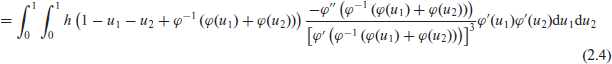
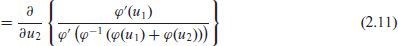
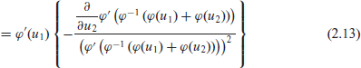
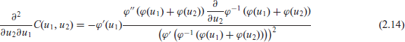
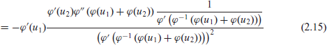
Proof. With an integrable function h defined on [0, 1]:

E (h (C^{*} (U_{1}, U_{2})))

= \int_{0}^{1} \int_{0}^{1} h (1 - u_{1} - u_{2} + C (u_{1}, u_{2})) d C (u_{1}, u_{2})

(2.3)

= \int_{0}^{1} \int_{0}^{1} h (1 - u_{1} - u_{2} + φ^{- 1} (φ (u_{1}) + φ (u_{2}))) \frac{- φ^{″} (φ^{- 1} (φ (u_{1}) + φ (u_{2})))}{{[φ^{'} (φ^{- 1} (φ (u_{1}) + φ (u_{2})))]}^{3}} φ^{'} (u_{1}) φ^{'} (u_{2}) d u_{1} d u_{2}

(2.4)

Writing $t_{1} = φ (u_{1}), t_{2} = φ (u_{2})$ , we have:

\begin{matrix} E (h (C^{*} (U_{1}, U_{2}))) = \int_{0}^{\infty} \int_{0}^{\infty} h (1 - φ^{- 1} (t_{1}) - φ^{- 1} (t_{2}) + φ^{- 1} (t_{1} + t_{2})) \frac{- φ^{″} (φ^{- 1} (t_{1} + t_{2}))}{{[φ^{'} (φ^{- 1} (t_{1} + t_{2}))]}^{3}} d t_{1} d t_{2} . \end{matrix}

(2.5)

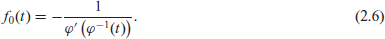
From the properties of the generator, $φ^{- 1}$ is decreasing with $φ^{- 1} \geq 0, φ^{- 1} (0) = 1, φ^{- 1} (\infty) = 0$ . Like $φ, φ^{- 1}$ is also continuous. Let us recall with Joe^[6] (p. 32) that these properties suffice to make $φ^{- 1} a$ survival function. Let $φ^{- 1} (t) = ℙ (T > t) = {\bar{F}}_{0} (t)$ for some random variable $T \geq 0$ . It has density

\begin{matrix} f_{0} (t) = - \frac{1}{φ^{'} (φ^{- 1} (t))} . \end{matrix}

(2.6)

Further,

\begin{matrix} - f_{0}^{'} (t) = - \frac{φ^{″} (φ^{- 1} (t))}{{(φ^{'} (φ^{- 1} (t)))}^{3}} \geq 0. \end{matrix}

(2.7)

So that $f_{0}$ is decreasing and

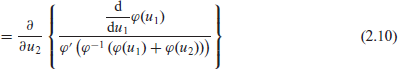
\begin{matrix} φ^{- 1} (t_{1} + t_{2}) = {\bar{F}}_{0} (t_{1} + t_{2}) = \int_{t_{1}}^{\infty} \int_{t_{2}}^{\infty} - f_{0}^{'} (s_{1} + s_{2}) d s_{1} d s_{2} . \end{matrix}

(2.8)

$- f_{0}^{'} (s_{1} + s_{2})$ is the joint density of $(φ (U_{1}), φ (U_{2}))$ on $[0, \infty) \times [0, \infty)$ . To see that, note first that the joint density of $(U_{1}, U_{2})$ is

\frac{\partial^{2}}{\partial u_{2} \partial u_{1}} C (u_{1}, u_{2}) = \frac{\partial}{\partial u_{2}} \frac{\partial}{\partial u_{1}} (φ^{- 1} (φ (u_{1}) + φ (u_{2})))

(2.9)

= \frac{\partial}{\partial u_{2}} \{\frac{\frac{d}{d u_{1}} φ (u_{1})}{φ^{'} (φ^{- 1} (φ (u_{1}) + φ (u_{2})))}\}

(2.10)

= \frac{\partial}{\partial u_{2}} \{\frac{φ^{'} (u_{1})}{φ^{'} (φ^{- 1} (φ (u_{1}) + φ (u_{2})))}\}

(2.11)

= φ^{'} (u_{1}) \frac{\partial}{\partial u_{2}} \frac{1}{φ^{'} (φ^{- 1} (φ (u_{1}) + φ (u_{2})))}

(2.12)

= φ^{'} (u_{1}) \{- \frac{\frac{\partial}{\partial u_{2}} φ^{'} (φ^{- 1} (φ (u_{1}) + φ (u_{2})))}{{(φ^{'} (φ^{- 1} (φ (u_{1}) + φ (u_{2}))))}^{2}}\}

(2.13)

\frac{\partial^{2}}{\partial u_{2} \partial u_{1}} C (u_{1}, u_{2}) = - φ^{'} (u_{1}) \frac{φ^{″} (φ (u_{1}) + φ (u_{2})) \frac{\partial}{\partial u_{2}} φ^{- 1} (φ (u_{1}) + φ (u_{2}))}{{(φ^{'} (φ^{- 1} (φ (u_{1}) + φ (u_{2}))))}^{2}}

(2.14)

= - φ^{'} (u_{1}) \frac{φ^{'} (u_{2}) φ^{″} (φ (u_{1}) + φ (u_{2})) \frac{1}{φ^{'} (φ^{- 1} (φ (u_{1}) + φ (u_{2})))}}{{(φ^{'} (φ^{- 1} (φ (u_{1}) + φ (u_{2}))))}^{2}}

(2.15)

= - φ^{'} (u_{1}) φ^{'} (u_{2}) \frac{φ^{″} (φ (u_{1}) + φ (u_{2}))}{{(φ^{'} (φ^{- 1} (φ (u_{1}) + φ (u_{2}))))}^{3}} .

(2.16)

Then, derive the density of $(T_{1}, T_{2}) = (φ (U_{1}), φ (U_{2}))$ as

- φ^{'} (φ^{- 1} (t_{1})) φ^{'} (φ^{- 1} (t_{2})) \frac{φ^{″} (t_{1} + t_{2})}{{(φ^{'} (φ^{- 1} (t_{1} + t_{2})))}^{3}} |det [\begin{matrix} \frac{1}{φ^{'} (φ^{- 1} (t_{1}))} & 0 \\ 0 & φ^{'} (φ^{- 1} (t_{2})) \end{matrix}]|

= - φ^{'} (φ^{- 1} (t_{1})) φ^{'} (φ^{- 1} (t_{2})) \frac{φ^{″} (t_{1} + t_{2})}{{(φ^{'} (φ^{- 1} (t_{1} + t_{2})))}^{3}} \times \frac{1}{φ^{'} (φ^{- 1} (t_{1})) φ^{'} (φ^{- 1} (t_{2}))}

(2.17)

= - \frac{φ^{″} (t_{1} + t_{2})}{{(φ^{'} (φ^{- 1} (t_{1} + t_{2})))}^{3}}

(2.18)

= - f_{0}^{'} (t_{1} + t_{2})

(2.19)

Further,

\begin{matrix} 1 - φ^{- 1} (t_{1}) - φ^{- 1} (t_{2}) + φ^{- 1} (t_{1} + t_{2}) = \int_{0}^{t_{1}} \int_{0}^{t_{2}} - f_{0}^{'} (s_{1} + s_{2}) d s_{1} d s_{2} . \end{matrix}

(2.20)

(Recall that $1 - ℙ (X_{1} > x_{1}) - ℙ (X_{2} > x_{2}) + ℙ (X_{1} > x_{1}, X_{2} > x_{2}) = ℙ (X_{1} \leq x_{1}, X_{2} \leq x_{2}))$

Thus,

\begin{matrix} E (h (C^{*} (U_{1}, U_{2}))) = \int_{0}^{\infty} \int_{0}^{\infty} h (1 - φ^{- 1} (t_{1}) - φ^{- 1} (t_{2}) + φ^{- 1} (t_{1} + t_{2})) (- f_{0}^{'} (t_{1} + t_{2})) d t_{1} d t_{2} . \end{matrix}

(2.21)

As any decreasing density on $[0, \infty)$ can be represented as a scale mixture of uniform densities (Williamson,^[7] $, f_{0} (t)$ is of the form

\begin{matrix} f_{0} (t) = \int_{t}^{\infty} \frac{d G (s)}{s} = \int_{t}^{\infty} \frac{g (s)}{s} d s, \end{matrix}

(2.22)

where G is a distribution function on $[0, \infty)$ , assumed to be absolutely continuous with density g. It is clear from Equation (2.7) that

\begin{matrix} g (t) = - t f_{0}^{'} (t) = - \frac{t φ^{″} (φ^{- 1} (t))}{{(φ^{'} (φ^{- 1} (t)))}^{3}} . \end{matrix}

(2.23)

With

a = \frac{t_{1}}{t_{1} + t_{2}} and b = t_{1} + t_{2},

E (h (C^{*} (U_{1}, U_{2}))) = \int_{0}^{\infty} \int_{0}^{1} h (1 - φ^{- 1} (a b) - φ^{- 1} ((1 - a) b) + φ^{- 1} (b)) g (b) d a d b

= 2 \int_{0}^{\infty} \int_{0}^{\frac{1}{2}} h (1 - φ^{- 1} (a b) - φ^{- 1} ((1 - a) b) + φ^{- 1} (b)) g (b) d a d b .

(2.24)

Let

ψ (a, b) = 1 - φ^{- 1} (a b) - φ^{- 1} ((1 - a) b) + φ^{- 1} (b) .

(2.25)

Fix a and let $ψ_{a} (b) = ψ (a, b)$ . As

ψ_{a} (b) = ℙ (φ (U_{1}) \leq a b, φ (U_{2}) \leq (1 - a) b) = ℙ (\frac{φ (U_{1})}{a} \leq b, \frac{φ (U_{2})}{1 - a} \leq b),

(2.26)

we have that $ψ_{a} (b)$ is increasing in b.

Put

ψ_{a} (b) = z \Leftrightarrow b = ψ_{a}^{- 1} (z) .

We can then rewrite Equation (2.24) as

E (h (C^{*} (U_{1}, U_{2}))) = 2 \int_{0}^{\frac{1}{2}} \int_{0}^{1} h (z) g (ψ_{a}^{- 1} (z)) (\frac{\partial}{\partial z} ψ_{a}^{- 1} (z)) d z d a for z \in [0, 1],

Hence, the density of $C^{*} (U_{1}, U_{2})$ is

\begin{matrix} k^{*} (z) = 2 \int_{0}^{\frac{1}{2}} g (ψ_{a}^{- 1} (z)) (\frac{\partial}{\partial z} ψ_{a}^{- 1} (z)) d a, where z \in [0, 1] . \end{matrix}

(2.27)

Corollary 2.1. $C^{*} (U_{1}, U_{2})$ has the same distribution as that of $1 - φ^{- 1} (W T) - φ^{- 1} ((1 - W) T) +$ $φ^{- 1} (T)$ where $(W, T)$ are independent, W has Uniform (0, 1) distribution and T has density g(.), whereas $C (U_{1}, U_{2})$ has the same distribution as that of $φ^{- 1} (T)$ .

In general, let $d \geq 2$ be an integer, and $(U_{1}, \dots, U_{d})$ be a d-tuple of standard uniform random variables whose joint distribution is given by a multivariate Archimedean copula C with generator $φ$ .

Let $T_{j} = φ (U_{j}), j = 1, \dots, d$ . Then, $(T_{1}, \dots, T_{d})$ has joint survival function $φ^{- 1} (t_{1} + \dots + t_{d})$ .

With $T = T_{1} + \dots + T_{d}, C (U_{1}, \dots, U_{d})$ is distributed as $φ^{- 1} (T)$ and $C^{*} (U_{1}, \dots, U_{d})$ is distributed as $1 + \sum_{j = 1}^{d} {(- 1)}^{j} φ^{- 1} (T_{1} + \dots + T_{j})$ .

However, a formula for the densities or simulation of C or $C^{*}$ does not seem to be tractable.

Remark 2.1. We can verify that $k^{*} (\cdot)$ is a probability density on [0, 1] by noting that since $g (\cdot)$ is a density on $[0, \infty)$ (see Equation (2.23)), we have

\int_{0}^{1} k^{*} (z) d z = 2 \int_{0}^{1 / 2} [\int_{0}^{1} g (ψ_{a}^{- 1} (z)) (\partial / \partial z ψ_{a}^{- 1} (z)) d z] d a = 2 \int_{0}^{1 / 2} [\int_{0}^{\infty} g (t) d t] d a = 2 \int_{0}^{1 / 2} d a = 1,

(2.28)

where we have used the change of variable $ψ_{a}^{- 1} (z) = t$ in the integral inside [...] and the fact that $ψ_{a}^{- 1} (\cdot)$ is an increasing function (in fact, a quantile function) with $ψ_{a}^{- 1} (0) = 0, ψ_{a}^{- 1} (1) = \infty$ for each $a, 0 < a < 1$ (see Equation (2.26)).

However, the quantile function $ψ_{a}^{- 1} (z)$ of the distribution of $(φ (U_{1}), φ (U_{2}))$ may not have a closed form expression, hindering the numeric applications.

Similarly to Barbe et al.^[5], we derive the limiting distribution of the Kendall process corresponding to $C^{*} (.,)$ . This is provided in the Theoren 2.2.

Theorem 2.2. Let

C_{n}^{*} (u_{1}, u_{2}) = \frac{1}{n} \sum_{i = 1}^{n} I \{U_{1 i} > u_{1}, U_{2 i} > u_{2}\}

be the empirical counterpart of $C^{*}$ and denote the distribution function of $C^{*}$ by $K^{*}$ .

Assume that (see Barbe et al.^[5])

(H.1) $K^{*} (.)$ .admits a continuous density $k^{*} (t)$ on $(0, 1]$ that verifies

\begin{matrix} k^{*} (t) = o \{t^{- \frac{1}{2}} {(log (\frac{1}{t}))}^{- \frac{1}{2} - ε}\} for some ε > 0 as t \to 0. \end{matrix}

(2.29)

(H.2) There exists a version of the conditional distribution of the vector $(U_{1}, U_{2})$ given $C^{*} (U_{1}, U_{2}) = t$ and a countable family $P$ of partitions $C$ of ${[0, 1]}^{2}$ into a finite number of Borel sets satisfying

\inf_{C \in P} \max_{C \in C} d i a m (C) = 0,

(2.30)

such that for all $C \in C$ , the mapping

\begin{matrix} t \mapsto μ_{t}^{*} (C) = k^{*} (t) ℙ \{(U_{1}, U_{2}) \in C ∣ C^{*} (U_{1}, U_{2}) = t\} \end{matrix}

(2.31)

is continuous on $(0, 1]$ with

\begin{matrix} μ_{1}^{*} (C) = k^{*} (1) I \{(0, 0) \in C\} \end{matrix}

(2.32)

Then the empirical process

α_{n}^{*} (t) = \sqrt{n} [\frac{1}{n} \sum_{i = 1}^{n} I \{C_{n}^{*} (U_{1 i}, U_{2 i}) \leq t\} - K^{*} (t)]

converges in distribution to a Gaussian process $α^{*}$ with 0 mean and covariance function

\begin{matrix} Γ* (s, t) = K^{*} (s \land t) - K^{*} (s) K^{*} (t) + k^{*} (s) k^{*} (t) R^{*} (s, t) - k^{*} (t) Q^{*} (s, t) - k^{*} (s) Q^{*} (t, s), \end{matrix}

(2.33)

Where

k^{*} (z) = 2 \int_{0}^{\frac{1}{2}} g (ψ_{a}^{- 1} (z)) (\frac{\partial}{\partial z} ψ_{a}^{- 1} (z)) d a for z \in [0, 1],

(2.34)

K^{*} (t) = \int_{0}^{t} k^{*} (z) d z for z \in [0, 1],

(2.35)

Q^{*} (s, t) = ℙ \{C^{*} (U_{1}) \leq s, U_{1} \geq U_{2} ∣ C^{*} (U_{2}) = t\} - t K^{*} (s),^{1}

(2.36)

and

R^{*} (s, t) = ℙ \{U_{1} \geq U_{2} \lor U_{3} ∣ C^{*} (U_{2}) = s, C^{*} (U_{3}) = t\} - s t,

(2.37)

with $U_{1} = (U_{1}^{(1)}, U_{1}^{(2)}), U_{2} = (U_{2}^{(1)}, U_{2}^{(2)})$ and $U_{3} = (U_{3}^{(1)}, U_{3}^{(2)})$ three independent copies of a random vector uniformly distributed in ${[0, 1]}^{2}$ and $\land$ denotes the componentwise minimum of the vectors.

Moreover, the limiting process has the following representation

\begin{matrix} α^{*} (t) = ν^{*} (A_{2, t}) - \int_{{[0, 1]}^{2}} ν^{*} (A_{1, u}) μ_{t}^{*} (d u), t \in [0, 1], \end{matrix}

(2.38)

with

A_{1, t} = \{u \in {[0, 1]}^{2} : u \geq t\}

(2.39)

A_{2, t} = \{u \in {[0, 1]}^{2} : C^{*} (u) \leq t\}

(2.40)

$ν^{*} :$ the (centred Gaussian) limit of the empirical process

\begin{matrix} v^{*} (A) = \sqrt{n} \{\frac{1}{n} \sum_{i = 1}^{n} I (U_{i} \in A) - ℙ (U_{i} \in A)\} \end{matrix}

(2.41)

for a set A of the form of $A_{1, t}$ or $A_{2, t}$ .

\begin{matrix} μ_{t}^{*} (d u) = μ_{t}^{*} (d u_{1}, d u_{2}) = \frac{d}{d u} k^{*} (t) [ℙ \{(U_{1} \leq u_{1}, U_{2} \leq u_{2}) \in C ∣ C^{*} (U_{1}, U_{2}) = t\}] . \end{matrix}

(2.42)

Remark 2.2. Note that variance of the limiting Gaussian process $α^{*} (\cdot)$ is

\begin{matrix} Γ* (t, t) = K^{*} (t) (1 - K^{*} (t)) + k^{*} (t) [k^{*} (t) R (t, t) - 2 t (1 - K^{*} (t))], \end{matrix}

(2.43)

since $Q^{*} (t, t) = t - t K^{*} (t)$ . This may be compared with the limiting variance for Kendall’s process obtained by Genest and Rivest^[3] as well as Barbe et al.^[5] (Theorem 2.1), namely,

\begin{matrix} Γ (t, t) = K (t) (1 - K (t)) + k (t) [k (t) R (t, t) - 2 t (1 - K (t))] . \end{matrix}

(2.44)

Thus Equation (2.43) is quite similar to Equation (2.44), with $(K, k)$ in the latter replaced by $(K^{*}, k^{*})$ in the former, as is to be expected.

Proof. $α_{n}^{*}$ can be decomposed as $α_{n}^{*} (t) = β_{n}^{*} (t) + γ_{n}^{*} (t)$ where

β_{n}^{*} (t) = \sqrt{n} [\frac{1}{n} \sum_{i = 1}^{n} I \{C^{*} (U_{1 i}, U_{2 i}) \leq t\} - K^{*} (t)]

and

γ_{n}^{*} (t) = \frac{1}{\sqrt{n}} \sum_{i = 1}^{n} [I \{C_{n}^{*} (U_{1 i}, U_{2 i}) \leq t\} - I \{C^{*} (U_{1 i}, U_{2 i}) \leq t\}]

It is then not hard to see that the proof of Theorem 5 of Barbe et al.^[5] holds in our case too.

In particular, the covariance function of $α^{*} (t)$ is obtained by computing the covariances

E \{v^{*} (A_{2, s}) v^{*} (A_{2, t})\} = ℙ \{C^{*} (U) \leq s \land t\} - ℙ \{C^{*} (U) \leq s\} ℙ \{C^{*} (U) \leq t\}

(2.45)

= K^{*} (s \land t) - K^{*} (s) K^{*} (t)

(2.46)

Next,

E \{v^{*} (A_{2, s}) \int_{{[0, 1]}^{2}} ν^{*} (A_{1, u}) μ_{t}^{*} (d u)\} = \int_{{[0, 1]}^{2}} ℙ \{C^{*} (U) \leq s, U \geq v\} μ_{t}^{*} (d v)

(2.47)

- \int_{{[0, 1]}^{2}} ℙ \{C^{*} (U) \leq s\} ℙ {U \geq v} μ_{t}^{*} (d v)

(2.48)

= k^{*} (t) Q^{*} (s, t)

(2.49)

Interchanging the roles of s and t, one also gets

E \{v^{*} (A_{2, t}) \int_{{[0, 1]}^{2}} v^{*} (A_{1, u}) μ_{s} (d u)\} = k^{*} (s) Q^{*} (t, s)

(2.50)

Finally,

E \{\int_{{[0, 1]}^{2}} ν^{*} (A_{1, u}) μ_{t}^{*} (d u) \int_{{[0, 1]}^{2}} ν^{*} (A_{1, u}) μ_{s}^{*} (d u)\}

(2.51)

= \int_{{[0, 1]}^{2}} \int_{{[0, 1]}^{2}} ℙ (U \geq u_{1} \lor u_{2}) μ_{s}^{*} (d u_{1}) μ_{t}^{*} (d u_{2})

(2.52)

- \int_{{[0, 1]}^{2}} \int_{{[0, 1]}^{2}} ℙ (U \geq u_{1}) ℙ (U \geq u_{2}) μ_{s}^{*} (d u_{1}) μ_{t}^{*} (d u_{2})

(2.53)

= k^{*} (s) k^{*} (t) R^{*} (s, t)

(2.54)

2.1. Examples

Let us illustrate our formula for the density of the survival distribution through some examples.

2.1.1 Independence Copula

The independence copula $C (u_{1}, u_{2}) = u_{1} u_{2}$ , where $u_{1}, u_{2} \in [0, 1]$ , has generator $φ (t) = - log (t), t \in$ $(0, 1]$ .

We calculate:

$φ^{'} (t) = - \frac{1}{t}, φ^{″} (t) = \frac{1}{t^{2}}, φ^{- 1} (t) = \exp (- t), for t \in (0, 1]$

$g (t) = t \exp (- t), for t \geq 0 (from Equation (2.23));$

$ψ_{a} (b) = 1 - \exp (- a b) - \exp (- (1 - a) b) + \exp (- b) = (1 - \exp (- a b)) (1 - \exp (- (1 - a) b)), for a \in [0, 1], b \in [0, \infty) .$

The density of $C^{*} (U_{1}, U_{2})$ is

k^{*} (z) = 2 \int_{0}^{\frac{1}{2}} ψ_{a}^{- 1} (z) exp (- ψ_{a}^{- 1} (z)) (\frac{\partial}{\partial z} ψ_{a}^{- 1} (z)) d a for z \in [0, 1] .

2.1.2. Clayton Copula

The Clayton copula

C_{θ} (u_{1}, u_{2}) = {(u^{- θ} + v^{- θ} - 1)}^{- \frac{1}{θ}}, for θ \in (0, \infty), u \in [0, 1], v \in[0, 1]

has generator

φ_{θ} (t) = \frac{1}{θ} (t^{- θ} - 1) with t \in (0, 1] .

Then:

$φ_{θ}^{'} (t) = - t^{- θ - 1}, φ_{θ}^{''} (t) = (θ + 1) t^{- θ - 2}, φ_{θ}^{- 1} (t) = {(θ t + 1)}^{- \frac{1}{θ}} for t \in (0, 1];$

$g_{θ} (t) = (θ + 1) t {(θ t + 1)}^{- 2 - \frac{1}{θ}} for t \geq 0 (from Equation (2.23));$

$ψ_{a, θ} (b) = 1 - {(θ a b + 1)}^{- \frac{1}{θ}} - {(θ (1 - a) b + 1)}^{- \frac{1}{θ}} + {(θ b + 1)}^{- \frac{1}{θ}} for a \in [0, 1], b \in [0, \infty) .$

The density of $C^{*} (U_{1}, U_{2})$ is

k^{*} (z) = 2 (θ + 1) \int_{0}^{\frac{1}{2}} ψ_{π, θ}^{- 1} (z) {(θ ψ_{σ, θ}^{- 1} (z) + 1)}^{- 2 - \frac{1}{t}} (\frac{\partial}{\partial z} ψ_{σ_{,} θ}^{- 1} (z)) d a for z \in [0, 1] .

2.1.3. Gumbel Copula

The Gumbel copula is

C_{θ} (u_{1}, u_{2}) = exp [- {({(- log (u_{1}))}^{θ} + {(- log (u_{2}))}^{θ})}^{\frac{1}{θ}}] for θ \in [1, \infty) .

Its generator is given by

φ_{θ} (t) = {(- log (t))}^{θ} where t \in [0, 1] .

Then:

$φ_{θ}^{'} (t) = - \frac{θ}{t} {(- \log (t))}^{θ - 1}, φ_{θ}^{''} (t) = \frac{θ}{t^{2}} {(- \log (t))}^{θ - 2} (- \log (t) + θ - 1), φ_{θ}^{- 1} (t) = \exp (- t^{\frac{1}{θ}}) for t \in (0, 1]$

$g_{θ} (t) = θ^{- 2} t^{\frac{1}{θ}} - 1 \exp (- t^{\frac{1}{θ}}) (t^{\frac{1}{θ}} + θ - 1) where t \geq 0 (from Equation (2.23));$

$ψ_{a, θ} (b) = 1 - \exp (- {(a b)}^{\frac{1}{θ}}) - \exp (- {((1 - a) b)}^{\frac{1}{θ}}) + \exp (- b^{\frac{1}{θ}}) for a \in [0, 1], b \in [0, \infty)$

The density of $C^{*} (U_{1}, U_{2})$ is

\begin{matrix} k^{*} (z) = 2 θ^{- 2} \int_{0}^{\frac{1}{2}} {(ψ_{a, θ}^{- 1} (z))}^{\frac{1}{θ} - 1} exp (- {(ψ_{a, θ}^{- 1} (z))}^{\frac{1}{θ}}) ({(ψ_{a, θ}^{- 1} (z))}^{\frac{1}{θ}} + θ - 1) (\frac{\partial}{\partial z} ψ_{a, θ}^{- 1} (z)) d a \\ for θ \in (1, \infty), z \in [0, 1] \end{matrix}

2.1.4. Ali-Mikhail-Haq Copula

The Ali-Mikhail-Haq copula

C (u_{1}, u_{2}) = \frac{u_{1} u_{2}}{1 - θ (1 - u_{1}) (1 - u_{2})} for θ \in [- 1, 1], u \in[0, 1], v \in[0, 1]

has generator

φ_{θ} (t) = log (\frac{1 - θ (1 - t)}{t}) with t \in [0, 1] .

Then:

$φ_{θ}^{'} (t) = - \frac{1 - θ}{t (1 - θ (1 - t))}, φ_{θ}^{''} (t) = \frac{(1 - θ) (1 - θ + θ t (2 - t))}{t^{2} {(1 - θ (1 - t))}^{2}}, φ_{θ}^{- 1} (t) = \frac{1 - θ}{\exp (t) - θ};$

$g_{θ} (t) = \frac{(1 - θ) t (\exp (2 t) - θ) \exp (t)}{{(\exp (t) - θ)}^{4}} (from Equation (2.23));$

$ψ_{a, θ} (b) = 1 - \frac{1 - θ}{\exp (a b) - θ} - \frac{1 - θ}{\exp ((1 - a) b) - θ} + \frac{1 - θ}{\exp (b) - θ} .$

The density of $C^{*} (U_{1}, U_{2})$ is

k^{*} (z) = 2 (1 - θ) \int_{0}^{\frac{1}{2}} \frac{ψ_{a, θ}^{- 1} (z) (exp (2 ψ_{a, θ}^{- 1} (z)) - θ) exp (ψ_{a, θ}^{- 1} (z))}{{(exp (ψ_{a, θ}^{- 1} (z)) - θ)}^{4}} (\frac{\partial}{\partial z} ψ_{a, θ}^{- 1} (z)) d a for θ \in [- 1, 1), z \in [0, 1] .

3. Illustration

In this section, we provide illustrations of our results.

3.1. Plots of $k^{*} (\cdot)$ for Some Copula Models

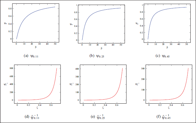
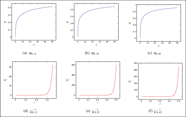
Figures 2 and 3 show graphics of the distribution function $ψ_{a}$ and the numerically estimated quantile function $({\hat{ψ}}_{a}^{- 1})$ of $B = φ (U_{1}) + φ (U_{2})$ for some values of $= \frac{φ (u_{1})}{φ (u_{1}) + φ (u_{2})}$ :

Figure 2.

Distribution Function $ψ_{a}$ and Its Estimated Inverse ${\hat{ψ}}_{a}^{- 1}$ for a = 0.11, a = 0.25 and, a = 0.45 in the Case of the Clayton Copula with $θ = I$ .

Figure 3.

Distribution Function $ψ_{a}$ and Its Estimated Inverse ${\hat{ψ}}_{a}^{- 1}$ for a = .011, a = 0.25, and a = 0.45 in the Case of the Gumbel Copula with $θ = 5$ .

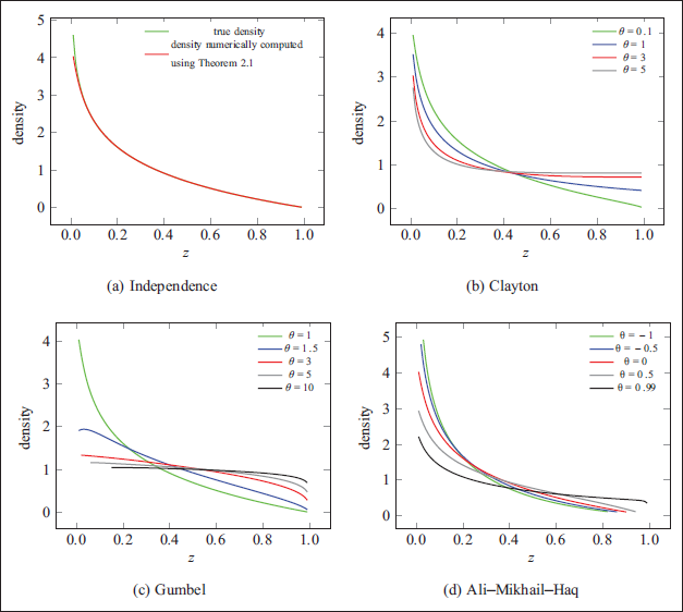
For the independence copula,

\begin{matrix} C^{*} (U_{1}, U_{2}) = (1 - U_{1}) (1 - U_{2}) = e x p (- log (1 - U_{1}) - log (1 - U_{2})) \end{matrix}

(3.1)

As U₁ and U₂ are uniformly distributed on [0, 1], it follows that $log (1 - U_{1}) + log (1 - U_{2}) \sim Γ (2, 1)$ (gamma distribution of shape 2 and scale 1) and $C^{*} (U_{1}, U_{2})$ has density

\begin{matrix} (- l o g (z)) e x p (- (- l o g (z))) \frac{1}{z} = - l o g (z), for z \in (0, 1] . \end{matrix}

(3.2)

Knowing the density of $C^{*}$ , we can evaluate in this case how our method performs (in Figure 4a).

Figure 4.

Density of $C^{*}$ for Some Archimedean Copulas.

Figures 4b-d show the density of $C^{*} (U_{1}, U_{2})$ for some Archimedean copulas:

3.2. Comparison of Simulated and Theoretical

k^{*} (\cdot)

, and Minimum Distance Estimation

With $U \sim U [0, 1], V \sim U[0, 1], (U_{1}, U_{2}) \sim C$ and $(U_{1}^{'}, U_{2}^{'})$ , an independent copy of $(U_{1}, U_{2})$ ,

C^{*} = C^{*} (U_{1}, U_{2}) = ℙ (U_{1}^{'} \geq U_{1}, U_{2}^{'} \geq U_{2} ∣ U_{1}, U_{2}) = ℙ (φ (U_{1}^{'}) \leq φ (U_{1}), φ (U_{2}^{'}) \leq φ (U_{2}) ∣ U_{1}, U_{2})

(3.3)

Taking advantage of the calculations in Section 2, we have

C^{*} = ℙ (φ (U_{1}) \leq W T, φ (U_{2}) \leq (1 - W) T ∣ W, T) = 1 - φ^{- 1} (W T) - φ^{- 1} ((1 - W) T) + φ^{- 1} (T),

(3.4)

where

W = \frac{φ (U_{1})}{φ (U_{1}) + φ (U_{2})} \sim U [0, 1] and T = φ (U_{1}) + φ (U_{2}) \sim G are independent.

T can be simulated by noticing that $φ^{- 1} (T) = S$ has density $k (s) = \frac{φ (s) φ^{″} (s)}{{(φ^{'} (s))}^{2}}$ for $0 \leq s \leq 1$ , which is of course the density of the Kendall distribution function $K (s)$ ; see Figures la-d. For example, the density of $S$ is $\frac{θ + 1}{θ} (1 - s^{θ}) ($ with $θ \in (0, \infty))$ for a Clayton copula and $- \frac{1}{θ} ln (s) + (1 - \frac{1}{θ}) ($ with $θ \in [1, \infty))$ for a Gumbel copula.

Then, from the simulated values of W and T, we can compute values of $C^{*}$ .

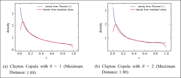
Figures 5a and b compare the densities obtained from application of Theorem 2.1 to those obtained from simulated values of $C^{*} (U_{1}, U_{2})$ for a Clayton copula:

Figure 5.

Comparison of the Density from Application of Theorem 2.I and the Density Simulated Using Corollary 2.1.

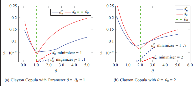
Figures 6a and b provide the plots $(θ, d_{n} (θ)), (θ, d_{n}^{*} (θ)$ , for the following distance-statistics:

d_{n} (θ) = max_{u} |K_{n} (u) - K_{θ} (u)|,

(3.5)

d_{n}^{*} (θ) = max_{u} |K_{n}^{*} (u) - K_{θ} (u)|,

(3.6)

where $K_{n} (\cdot), K_{n}^{*} (\cdot)$ are the empirical distribution functions of $C_{n} (U_{1 i}, U_{2 i})$ and $C_{n}^{*} (U_{1 i}, U_{2 i}), 1 \leq i \leq n$ , respectively, $K_{θ} (\cdot)$ is the Kendall function given in Equation (1.4), and $K_{θ}^{*} (\cdot)$ is given in Equation (2.35). Here we have used the Clayton copula model to simulate ( $U_{1 i}, U_{2 i}), 1 \leq i \leq n$ , as well as to compute $K_{θ}$ and $K_{θ}^{*}$ . The minimizers of the plots may be used as estimates of $θ$ . This illustrates a possible use of our result for inference purposes.

Figure 6.

Distance Statistics (n = 197).

4. Conclusion

Inspired by the importance of Kendall functions for identifying Archimedean copula models, we decided to examine the distribution of the survival functions from Archimedean copulas in this article. We were able to derive a formula for the density. This was achieved by observing that $C^{*} (U_{1}, U_{2})$ has the same distribution as $1 - φ^{- 1} (W T) - φ^{- 1} ((1 - W) T) + φ^{- 1} (T)$ where W and T are independent, W has a uniform distribution on (0, 1) and T is from some density g(.). Moreover, the approach used allows the derivation of the limiting behaviour of the empirical Kendall process and a representation that is useful in simulating the values of the survival distribution function of copulas. However, the difficulty in finding an analytical form of quantile functions in general limits the reach of the formula.

Footnotes

Acknowledgements

The authors would like to thank the referees and the Associate Editor for their critical comments that led to an improved version of the article.

Declaration of Conflicting Interests

The material in this article is from the PhD thesis of Magloire Loudegui Djimdou, submitted to Concordia University. Consequently, there are substantial overlaps between the thesis and the article. As per Concordia rules, the thesis has been archived in a repository called Spectrum at Concordia University by the author (https://spectrum.library.concordia.ca/id/eprint/990063/). The author has full copyright as per the rules of the copyright at Spectrum, as Concordia University does not claim copyright over anything deposited in Spectrum and is therefore free to use any part of the thesis in any of his future publications.

Funding

The author disclosed receipt of the following financial support for the research, authorship, and/or publication of this article: The research of Y. Chaubey and A. Sen was supported by the Natural Sciences and Engineering Research Council (NSERC), Canada.

Note

ORCID iD

Magloire Loudegui Djimdou

References

Sklar

Fonctions de répartition à n dimensions et leurs marges. Publications de l'Institut de Statistique de l'Université de Paris 1959; 8: 229–231.

Chakak

and Ezzerg

Bivariate contours of copula. Commun Stat Simul Comput 2000; 29 (1): 175–185.

Genest

and Rivest

L-P.

Statistical inference procedures for bivariate Archimedean copulas. J Am Stat Assoc 1993; 88(423): 1034–1043.

Genest

, Quessy

J-F

and Rémillard

Goodness-of-fit procedures for copula models based on the probability integral transformation. Scand J Stat 2006; 33: 337–366.

Barbe

, Genest

, Ghoudi

, . On Kendall’s process. J Multivar Anal 1996; 58(2): 197–229.

Joe

Dependence modeling with copulas . CRC Press 2014.

Williamson

RE.

Multiply monotone functions and their Laplace transforms. Duke Math 1956; 23: 189–207.

Distribution of the Joint Survival Function of an Archimedean Copula

Abstract

Keywords

1. Introduction

Density k z , z ∈ 0 , I , of the Kendall Distribution for Some Archimedean Copulas.

Examples of Archimedean Copulas.

2.1.1 Independence Copula

2.1.2. Clayton Copula

2.1.3. Gumbel Copula

2.1.4. Ali-Mikhail-Haq Copula

3. Illustration

3.1. Plots of k * ( ⋅ ) for Some Copula Models

Figure 2.

Distribution Function ψ a and Its Estimated Inverse ψ ^ a − 1 for a = 0.11, a = 0.25 and, a = 0.45 in the Case of the Clayton Copula with θ = I .

Distribution Function ψ a and Its Estimated Inverse ψ ^ a − 1 for a = .011, a = 0.25, and a = 0.45 in the Case of the Gumbel Copula with θ = 5 .

Density of C * for Some Archimedean Copulas.

Comparison of the Density from Application of Theorem 2.I and the Density Simulated Using Corollary 2.1.

Distance Statistics (n = 197).

Footnotes

Acknowledgements

Declaration of Conflicting Interests

Funding

Note

ORCID iD

References

Density $k (z), z \in (0, I)$ , of the Kendall Distribution for Some Archimedean Copulas.

3.1. Plots of $k^{*} (\cdot)$ for Some Copula Models

Distribution Function $ψ_{a}$ and Its Estimated Inverse ${\hat{ψ}}_{a}^{- 1}$ for a = 0.11, a = 0.25 and, a = 0.45 in the Case of the Clayton Copula with $θ = I$ .

Distribution Function $ψ_{a}$ and Its Estimated Inverse ${\hat{ψ}}_{a}^{- 1}$ for a = .011, a = 0.25, and a = 0.45 in the Case of the Gumbel Copula with $θ = 5$ .

Density of $C^{*}$ for Some Archimedean Copulas.