
Abstract
The Director of the US Census Bureau every five years, under the Voting Rights Act (VRA) Section 203(b), determines which states and political subdivisions must provide ballot assistance in languages other than English. These rule-based determinations use small-area estimates of the proportions of voting-age citizen members of racial/ethnic Language Minority Groups (LMGs) who are limited Englishproficient (LEP) and of LEP LMG persons who are also illiterate. This large-scale Small Area Estimation (SAE) effort by the US Census Bureau is based on American Community Survey five-year data. This paper focuses on the unique attributes of this SAE problem, including the predominance in each LMG of tiny domains along with relatively few large domains that account for the bulk of LMG citizens. The data and small area models are treated separately for distinct LMGs, and the spirit of the law requires that the domain estimates should be produced in a similar way across LMGs for each type of geography (Jurisdictions, which are mostly counties, plus two types of American Indian and Alaskan Native areas). The paper describes and assesses the SAE models developed under unique constraints, including novel methodological aspects and the use of hybrid frequentist and Bayesian computational techniques; situates these modelling choices in the broader literature on SAE; and discusses the strengths and weaknesses of the resulting models.
Keywords
Introduction
According to Section 203(b) of the U.S. Voting Rights Act (VRA) of 1965 beginning in 1975, states and political subdivisions must in certain circumstances make voting materials available in languages other than English. Section 203(b) prescribes that the Director of the US Census Bureau shall make these coverage determinations every five years, based on the most current population estimates derived from the American Community Survey (ACS) five-year data along with relevant census data. These determinations are based on estimates of voting-age citizen subgroups defined by race and language proficiency in States and local geographic areas called Jurisdictions, American Indian Areas (AIAs), and Alaskan Native Regional Corporations (ANRCs). Jurisdictions are Counties in all but eight states and Minor Civil Divisions in the other states.
The 2021 determinations (Census RVRDO)[6] were based on the 2015-2019 five-year ACS data. These data contain at least one voting-age respondent in 7,859 Jurisdictions, 568 AIAs, and all 12 ANRCs. The racial and ethnic self-identifications of census or ACS respondents in these geographies are used to define 73 Language Minority Groups’ (LMGs). Of the LMGs eligible in 2021, 21 are Asian, 51 are American Indian or Alaska Native (AIAN) and 1 is Hispanic.
Within the LMGs, Section 203(b) categorizes voting-age persons according to responses to ACS questions regarding citizenship, limited English proficiency and illiteracy. Limited English-proficiency is defined as speaking a language other than English at home and speaking English less than very well’. Illiteracy is defined as having less than a fifth grade education. Throughout this paper, we refer to the relevant nested population subgroups by the following abbreviations:
VOT: Voting-age persons; CIT: Voting-age citizens; LEP: Limited English-proficient, voting-age citizens; and ILL: Illiterate, limited English-proficient, voting-age citizens.
VRA Section 203(b) coverage determinations for states and political subdivisions depend according to specific rules on estimates and ratios of estimates of the CIT population within geographic areas and of subpopulations LEP and ILL within geographic areas intersected with LMGs (Census RVRDO)[6]. The rules for the determinations are specified in the data-release documents and Technical Report Slud et al.[32], Appendices A-B. The estimates underlying determinations for each LMG must depend on data for only that LMG, but the techniques for producing the estimates should be similar across LMGs.
In this Introduction, we explain the rationale and properties of model-based small area estimates of the various population counts needed for VRA determinations. To fix terminology and notations, we restrict attention only to the Jurisdiction geography-type.
VRA Section 203 Determinations as a Statistical Problem
Within each LMG (labelled g) and geographic unit (jurisdiction, labelled j), the primary ACS data consist of a sample of
To mitigate this small-domain imprecision, starting in 2011 (Joyce et al.)[14, 15] and also in 2016 (Slud et al.)[31] and 2021 (Slud et al.)[32], the Census Bureau embarked on a research and development effort to produce domain population estimates and ratios supporting the VRA Section 203 determinations via model-based analyses of ACS - and, if possible, decennial census - data. This research on improving the estimates supporting the Section 203(b) determinations has been conducted within a framework of model-based Small Area Estimation (SAE). The main idea of SAE is that many small (GLMG) domains within the same LMG may behave similarly with respect to domain proportions of CIT within the VOT population, of LEP within CIT and of ILL within the LEP population. This similarity may manifest itself within each LMG in the form of shared relationships and model parameters between the outcome proportions, observable domain-specific covariates, and similarly distributed random effects distinguishing jurisdictions. In the 2016 formulation the random probabilities
Separate models were estimated for each LMG across jurisdictions, and also for each AIAN LMG across AIAs and again across ANRCs. Guided by the principle of analysing each combination of LMG and geography type separately, since 2016 each model has been fitted from data on all voting-age persons within the LMG regardless of their membership in other LMGs. The only way in which models fitted to different LMGs influence one another is that the subset of fixed-effect covariates used for an LMG in each geography type was chosen from a list of possible predictors according to a grouping of LMGs with similar numbers of (Geo, LMG) domains containing ACS samples.
As in most SAE projects, an important first goal was to document the improvement in accuracy of the resulting model-based estimates over the estimates that would have arisen through purely survey-weighted estimates (called design-based’ or direct’ estimates) that do not rely on models of relationships between outcome variables or between outcomes and auxiliary data such as administrative records. In the 2011 and 2016 cycles of the VRA project, this was done exclusively by displaying the extent to which variances (or Mean-Square Prediction Errors in the empirical Bayes models) are smaller, domain by domain, for the model-based estimates versus the direct estimates. That was neither true in all (Geo, LMG) domains, nor was it expected to be, but it was true for most domains. Similarly, analysis in the 2021 cycle Slud et al.[32] demonstrated the same kind of systematic but not universal variance improvement for the model-based estimates over their direct survey-weighted analogues. But the 2021 analysis had the further goals of examining model adequacy and of comparing the quality of estimates across different (Bayesian versus frequentist) estimation techniques with the aid of diagnostics. In the absence of ground truth, it has been necessary to rely on diagnostics comparing aggregated estimates versus aggregated direct estimates, since the direct estimates in a high-quality, high response-rate survey like the ACS are nearly unbiased, and these estimates are therefore reliable on domains with large sample. In a limited way, model adequacy was investigated in 2016 (Ashmead and Slud)[2] using model-based reference distributions determined by parametric bootstrap in empirical Bayes SAE.
Thus, the goals of the SAE analysis in the VRA Section 203(b) project are improved accuracy over direct estimates and careful model assessment, and the goals of this paper are to display both with emphasis on SAE methodological validity and novelty. The paper addresses the question of whether and in what way the covariates were useful across a range of LMGs of radically different sizes. Similarly, we study whether and how the models with the most detailed random effects parameterizations can be documented to outperform those with simpler, independent random effects for the three successive outcomes CIT within VOT, LEP within CIT, and ILL within LEP.
Special Features of SAE in the VRA Section 203(b) Project
The SAE problem described here has several distinctive features that partially dictate the models and methods used. There were 7,859 jurisdictions with an ACS sample in 2015-2019, further broken down by LMG, and the great majority of (Geo, LMG) domains were very small. Partly for that reason, the available predictive covariates were very weak, as summarized in Section 2.3 and discussed fully in the Technical Report Slud et al.[32] (Section 2.3).
The number of (Geo, LMG) domains with a voting-age sample varies widely across LMGs. There are 76 LMGs, after breaking the Hispanic LMG into four (numbered 73-76) by Census Region. Most LMGs have fewer than 100 jurisdictions with a voting-age sample size >10 but the largest 10 LMGs have hundreds of jurisdictions with a sample > 100. The numbers of jurisdictions with the same minimum sample sizes of LEP persons was much smaller. The largest LMGs have hundreds of jurisdictions with LEP samples > 20, but the smallest 30 LMGs have fewer than 100 jurisdictions with LEP sample size > 3. The tremendous imbalance between the numbers of very low-sample (Geo, LMG) domains and of moderate-to-large ones plays a dominating role in the kinds of models that can be fitted and in their diagnostic model assessments. Supplement Figure S1(a)-(b) show for LMGs ordered by decreasing population the log number of jurisdictions with at least k sampled persons, respectively for voting-age and LEP persons, for several values of k.
Some of the special features that make the SAE problem in VRA Section 203(b) unique are:
Nested decreasing outcome categories CIT, LEP, ILL within VOT; A large number of parallel SAE analyses for domains within LMGs (73 LMGs for all jurisdictions, 51 AIAN LMGs for AIAs and for ANRCs) ranging from very data-rich to data-sparse: Analyses should be similar with respect to model type across (large groups of) LMGs, but data analyses in distinct LMGs must be separate; Great predominance in each LMG of geographic units with sample size < 5, among which many counts of 0 LEP and ILL outcomes are observed; Domain-specific covariates are extremely weak, derived from higher-level survey estimates.
Many SAE problems have feature (i), and some with feature (iv) produce estimates primarily exhibiting empirical Bayes shrinkage. Large statistical agencies often see small-domain datasets with features (ii) (iii), although those datasets seldom lead to useful small area estimates unless, as in the Census Bureau’s Small Area Income and Poverty Estimates (SAIPE) programme, the predictive covariates are very strong (Maples)[21].
This paper outlines models and analytical tools motivated by features (i)-(iv). It introduces novel methodological wrinkles combining frequentist and Bayesian techniques and demonstrates that the resulting SAE estimates are sensible and clearly superior to the direct survey-weighted estimates. The remainder of the paper is organized as follows. The next section describes SAE methodology leading up to the MLN models used in production, along with an SAE literature review placing those models in context and a description of predictive covariates. Section 3 contains several comparisons: (1) SEs for SAE model estimates versus directed survey-weight estimates, (2) predictions obtained by three different SAE calculations within related MLN models, (3) aggregated predictions from MLN models versus the unbiased aggregated direct survey estimates and (4) predictions and run-times for Bayesian versus frequentist estimates within the same MLN model. Then a concluding section discusses our findings, limitations of the SAE models used to produce estimates, and new directions for methodological research in this SAE problem.
Section 203(b) of the VRA requires that a geographic unit (jurisdiction, AIA or ANRC) provide ballot assistance in a language other than English in part as a function of the estimated proportions of LMG LEP citizens among the citizens of the geographic unit, or of LMG ILL citizens among the LMG LEP citizens of the geographic unit. There is another way to trigger’ ballot language assistance, in jurisdictions with more than 10,000 LEP citizens, but such jurisdictions have a large enough sample that direct estimates are sufficiently accurate to estimate domain counts. The focus in VRA on proportions of LMG citizens in the successive nested categories CIT, LEP, and ILL motivates a nested, hierarchical structure for all SAE model classes considered. That is, any joint SAE model used to describe the data should incorporate an interpretable covariate-based random-effect model for the (Geo, LMG) count of CIT outcomes within the VOT (Geo, LMG) domain, and similarly should incorporate models for the LEP outcome within the CIT (Geo, LMG) domain and for the ILL outcome within the LEP (Geo, LMG) domain. These conditional models represent counts of outcome a + 1 within the (Geo, LMG) domains of outcome a, for a = 0,1,2. Neither the domain (j, g) VOT counts
SAE Literature Review
SAE aims to improve domain predictions relative to direct survey estimates by borrowing strength from similar domains and auxiliary data through shared model parameters (Rao and Molina)[28]. The specific interest here is in SAE models, such as multinomial logistic models, that can handle categorical outcomes. The general reference Agresti[1] (Section 13.2-13.4), not focused on SAE, treats logistic-normal and other mixed-effect multinomial regression models, while the paper Jiang and Lahiri[13] (Section 4) covers multinomial regression models in SAE from the general viewpoint of mixed-effect generalized linear models. The Dirichlet multinomial model, mentioned in textbooks as generalizations of the BetaBinomial (Carlin and Louis[5]; Agresti[1]), has also been used in SAE for categorical responses in Census Bureau research (Slud et al.[31]; Maples[21]).
Other authors have used MLN models for SAE. A seminal early work Ghosh et al.[12] treated hierarchical generalized linear mixed-effect models for SAE with unit-level data. SAE papers studying area-level MLN models include Molina et al.[24] López-Vizcaíno et al.[18]; López-Vizcaíno et al.[19]; the first of these papers applied an MLN model with one shared random effect across employment categories, and the third also included the temporal structure of the random effects. The latter two papers include distinct random effects across multinomial categories, but their assumption that random effects are independent within each area would be unrealistic in many settings. Some articles (Saei and Taylor[29]; Scealy[30]) used MLN with dependent random effects, but their models handled only three categories, and the extension to more categories is not straightforward (Dawber et al)[8].
The paper Parker et al.[25] provides a different Bayesian implementation of unit-level models, using variational Bayes computations. It also incorporates pseudo-likelihood adjustments to account for possible informative sampling, which is important for unit-level models. Despite achieving computational efficiency for a unit-level model, this approach might be computationally expensive relative to area-level SAE. Unit- and area-level models each have advantages and disadvantages (Franco and Maitra)[10].
The MLN regression parameterization used here for SAE in the VRA application (Slud et al.)[32] is particularly suited to the nested outcomes CIT, LEP and ILL but differs from other parameterizations in the SAE literature. This is the continuation-ratio logit’ (Agresti) [1] (Section 8.3.6) that is most often applied to longitudinal or survival data and was introduced into mixed-effect MLNs by Coull and Agresti [7]. This parameterization has been used in a Dirichlet multinomial SAE model (Slud et al.)[31], both in the usual version and in a variant with a dispersion parameter varying linearly with the square root of domain sample size. Within the general continuation-ratio MLN models, the multi-category Gaussian random effects can be dependent. A published data illustration (Coull and Agresti)[7] performed likelihood ratio tests (LRTs) for various submodels but not for the hypothesis of independent random effects; however, our experience (Slud et al.)[32] (Section 3.5) suggests that in SAE applications with multiple nested categories, the MLN model with independent random effects across categories may often be adequately general.
SAE literature contains a few other proposals for handling categorical outcome data. As an extension of the work (Liu et al.[17]), the paper (Wang et al.[35]) assumes the standard design-based estimators of proportions follow a generalized Dirichlet distribution. However, continuous distributions are not always appropriate for discrete quantities that have a large number of zeros and may cause problems when implementing MCMC. A completely different unit-level proposal was based on expectile regression (Dawber et al.[8]: although computationally efficient when there are many categories, its estimates have not been shown to be design-consistent, and it does not account for informative sampling.
Computational Issues
There is a large literature on statistical computing of the Bayesian MCMC and frequentist MLE estimates discussed in this paper. On the Bayesian side, our general references are the
During much of the period during which frequentist MLN models were explored in the SAE literature, the computation of mixed-effect MLN regression models was considered difficult (Jiang and Lahiri)[13] (Section 4.3.1). That is no longer true, due to Adaptive Gaussian Quadrature (AGQ) algorithms (Pinheiro and Bates)[26], which are implemented on many statistical computing platforms including
Model Description
The VRA problem setting is expressed in terms of a succession of proportions CIT/VOT, LEP/CIT and ILL/LEP of the populations in (Geo, LMG) domains. In the notation of the Introduction, these are proportions

where
The direct (i.e., survey-weighted) estimated counts

These response variables are in general not integers, although their successive differences are modelled below as multinomial random variables, with parameters estimated using likelihood expressions which make mathematical sense but are not actually likelihoods for non-integer responses.
We next present the models used and considered in past and present cycles of SAE in the VRA context. First express the response data for mutually exclusive rather than nested outcome categories (VOT not CIT, CIT not LEP, LEP not ILL, and ILL) in the form

The multinomial regression model has the form

where
The Dirichlet multinomial model used in the VRA project in 2016, similar in spirit but not in detail to the one used in 2011, was (2.3) with

where the fixed-effect rates

and the unknown parameters are
The MLN model with similar fixed-effect parameterization takes the form (2.3) with

where the random effect triples

The Appendix summarizes the different mathematical notations and assumptions used in these random-effect models and relates them to the random true-population ratios
If in (2.3) and (2.5) or in (2.6) the random effects
Model (2.3)-(2.4) can also be presented as successive conditional models. Using well-known properties of the Dirichlet distribution it is shown to be precisely equivalent to the models
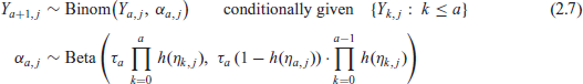
in the special case where
In the process of model-building in Slud et al.[32] (Section 3.2), predictions based on maximum likelihood fits of parameters in the Dirichlet multinomial model (2.7) were compared with those in MLN-D. The MLN-D model was found to perform better with respect to simple diagnostics, and further analyses and production of estimates for the 2021 VRA determinations were done only with the MLN-D and MLN-F models.
Covariates from administrative records were not available when the model was developed. Instead, covariates from ACS were computed from the same ACS 2015-2019 dataset as the domain response variables, but at higher levels of aggregation. This was done to mitigate problems of measurement error, which can cause suboptimal predictions and misspecification of uncertainty measures (Ybarra and Lohr [36]; Bell et al.[4]) In addition, the sample overlap between the response and the covariate at a higher level of aggregation was removed. Overlap in the sample induces dependence between the sampling and model errors which contradicts the conditional independence assumptions of MLN and other area-level models.
For the 2021 determinations based on the ACS data, one set of covariates was defined as the higher-geography-level LMG proportion of CIT within VOT, LEP within CIT, and ILL within LEP, in the portion of the State complementary to a Jurisdiction it contains, or the portion of the whole AIAN LMG complementary to an AIA. All other covariates were defined at the level of the geographic unit, without regard to LMG. One such covariate
Results on Performance of Modeled Estimates
Whether counts are estimated by direct or model-based methods, the uncertainty in SAE can be quantified by the conditional or unconditional expected square discrepancy (MSPE) between the estimate and the target. Subtle differences between these notions arise depending on whether we regard the target totals as being pure counts or stochastic, modelled quantities. See the Supplement, Section S1, for the connection between model random effects and true domain populations.
The estimation and uncertainty measurement arises for the survey-weighted direct estimators
When assessing model-based SAE estimation or prediction errors, the targets are random, and there is a distinction between the unconditional and conditional expectation of
Throughout this paper, variances’ or MSPEs for direct or model-based frequentist estimates are reported as unconditional MSPEs derived from SDR, while conditional MSPEs for Bayesian estimates are reported as MCMC-based posterior variance estimates. The detailed discussion of the differences between these variance and MSPE concepts is given in Section D.1 of the Technical Report Slud et al.[32].
The (Geo, LMG) estimates for 2021 determinations in jurisdictions were produced in two different ways. For the 24 largest LMGs, those for which there were at least 700 jurisdictions with any ACS sample, the parameter estimates, domain predictions and posterior variances were computed under model MLN
For the LMGs other than the largest 24, parameters were computed via frequentist MLEs, and domain predictions and SDR based mean-squared prediction error (MSPE) estimates were derived from those. For purposes of comparison, in nine large LMGs for which the production estimates were Bayesian, parameter estimates and domain predictions and MSPEs were re-computed using frequentist MLEs and prediction formulas under both models MLN-D and MLN-F.
The subsections that follow explore data-analytically different aspects of the direct and MLN model-based predictions. Section 3.1 focuses on SEs of direct versus MLN production estimates in jurisdictions, across all LMGs. The remaining subsections restrict attention to nine LMGs (eight Asian and NE regional Hispanic) for which direct, frequentist MLN-D and MLN-F, and Bayesian MLN-F estimates are all available. Section 3.2 explores MLN-D versus MLN-F predictions, whether those predictions came from Bayes or frequentist analysis. Section 3.3 uses diagnostics to assess the quality of fitted models, and Section 3.4 compares Bayes versus frequentist predictions, SEs, and computation times.
MSPE Comparisons
Three types of estimates and SEs were considered for
We first address the frequency of improvement of variability of the estimates in single domains, by comparing direct to model-based estimates of SEs and CVs. Larger SEs or CVs imply a higher degree of uncertainty, and therefore worse estimation performance. For most comparisons, we omit estimates with direct-method SE estimates of 0. In some cases, we omit estimates based on VOT sample size < 5, both because such estimates are unreliable and because samples this small only rarely result in Section 203(b) determinations. Exhibits are created from all (Geo, LMG) domains meeting the stated criteria.
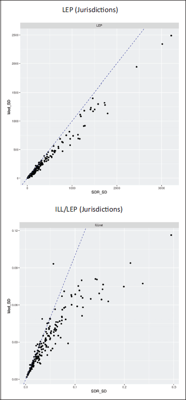
The scatterplots in Figure 1 show the relationship between direct (SDR) and model-based SEs for single (Geo, LMG) domains for the variables LEP and ILL/LEP. In each plot, SDR and model-based SEs would be equal along the dashed blue line. Points below [above] the line indicate domains for which the direct-estimated SE is larger [smaller] than the corresponding model-based estimate. Domains for which either the SDR or (frequentist) model SEs are estimated as zero are not meaningful, and have been omitted. To reduce visual clutter, and emphasize relevance to VRA determinations, the plots are restricted to domains with
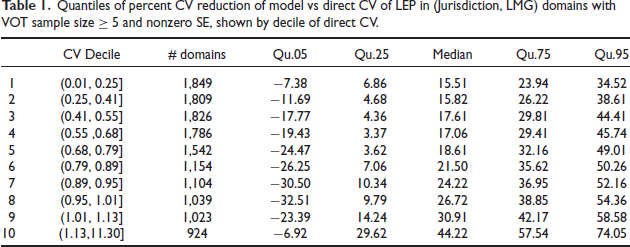
Table 1 and Supplement Table S. 1 confirm the same point, respectively for estimates of LEP and of ILL/LEP ratios, by displaying quantiles of the percent reduction of model versus direct CVs by decile of the direct estimated CV. The tables tally only domains for which both the model and SDR SEs are positive. In both tables, the median percent reduction of CV is positive (> 9%), that is, the model-based CV is typically lower than the direct CV. For LEP estimates, the median reduction is similar in most of the direct CV bins, except in the largest deciles which show the largest reduction. The range of LEP CV reductions is seen to increase with direct CV. In contrast, the median reduction of the ILL/LEP CVs increases systematically across all deciles of the direct CVs: the higher the direct CV, the larger appears the benefit of the model-based estimate.
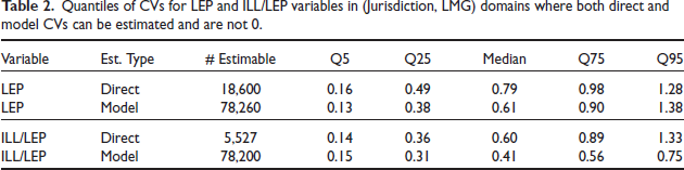
Another advantage of model-based estimates is that direct-method CVs often cannot be calculated for domains where the sample is too small to estimate both the standard deviation and mean, while model-based CVs are estimable. Table 2 (third column) shows the numbers of (Geo, LMG) domains with estimable CVs for direct and model-based estimates of LEP and ILL/LEP and compares quantiles of the model and direct CV estimates in domains where both can be calculated. In those domains, the model-based CVs tend to be lower than the direct CVs for both LEP and ILL/LEP. The diagnostics shown above all support the conclusion that the model SE estimates are generally smaller than the direct SDR estimates of standard deviation for both LEP and ILL/LEP. The model-based Section 203(b) estimates are more accurate in that sense than the direct survey-weighted estimates.
Quantiles of percent CV reduction of model vs direct CV of LEP in (Jurisdiction, LMG) domains with VOT sample size ≥ 5 and nonzero SE, shown by decile of direct CV.
Quantiles of CVs for LEP and ILL/LEP variables in (Jurisdiction, LMG) domains where both direct and model CVs can be estimated and are not 0.
The statistical adequacy of MLN-D as a submodel of MLN-F can be tested using LRT. The parameter dimension of MLN-D is smaller by three, corresponding to the above-diagonal entries of the covariance matrix
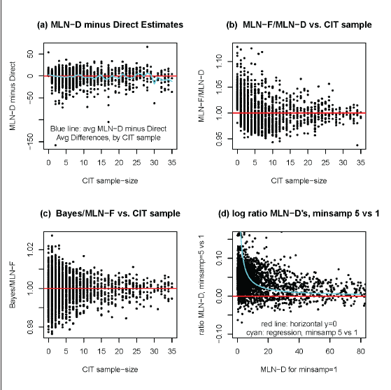
Comparison of LEP estimates in 2966 LMG4 jurisdictions with CIT sample ≤ 35. (a) Differences between MLN-D and Direct estimates. Blue line is average difference for jurisdictions with specified CIT sample sizes. (b) Ratio of MLN-F over MLN-D LEP estimates for jurisdictions, plotted by CIT sample-size. (c) Ratio of Bayes over frequentist MLN-F LEP estimates, plotted by CIT sample-size. (d) Ratio of MLN-D estimates fitted on all jurisdictions with VOT sample (minsamp = 1) vs. MLN-D estimates fitted on jurisdictions with VOT sample ≥ 5 (minsamp = 5), plotted vs. minsamp = 1 estimates.
Comparison of LEP estimates in 2966 LMG4 jurisdictions with CIT sample ≤ 35. (a) Differences between MLN-D and Direct estimates. Blue line is average difference for jurisdictions with specified CIT sample sizes. (b) Ratio of MLN-F over MLN-D LEP estimates for jurisdictions, plotted by CIT sample-size. (c) Ratio of Bayes over frequentist MLN-F LEP estimates, plotted by CIT sample-size. (d) Ratio of MLN-D estimates fitted on all jurisdictions with VOT sample (minsamp = 1) vs. MLN-D estimates fitted on jurisdictions with VOT sample ≥ 5 (minsamp = 5), plotted vs. minsamp = 1 estimates.
The overall conclusions of these comparisons are that in many but not all large LMGs, the MLNF models are barely significantly different from the MLN-D models, and when the LRT statistic is significant, the MLN-F model parameter estimates and SAE predictions are essentially the same whether made by Bayesian or frequentist computations. Further comparisons between the computational burdens of the frequentist (MLN-D or MLN-F) and Bayesian (MLN-F) analyses are given in Section 3.4.
Panels (a) in Figure 2 and Supplement Figure S4 point to possible flaws in the small-sample model predictions that we explore further in diagnostic tables assessing the goodness of fit of these models. Close examination of panels (a) in these figures shows a slight tendency for the average MLN-D predictions minus direct ACS weighted estimates within CIT sample size groups to be positive for sample sizes < 3 and negative for jurisdictions with CIT sample-size in the range 3-35. These differences may seem trivial for each single CIT sample size, but as Figure S.1 shows, the great majority of jurisdictions have very small sample sizes. When the MLN-D predictions are aggregated versus the direct ACS estimates for LEP or ILL over jurisdictions defined by intervals of CIT sample size, the population groups have large total sample size and the (roughly unbiased) ACS estimates are expected to be accurate, and so can be used to assess the MLN-D predictions. These aggregated comparisons are shown in Supplement Tables S2 and S3, which confirm in detail for both LMGs 4 and 9 the patterns seen for LMG 4 in Figure 2.
In LMG 4, the aggregated MLN-D estimates for LEP counts are larger than the direct estimates when CIT sample size is
What might cause this pattern of model-based over-estimation in very small-sample jurisdictions and under-estimation in jurisdictions with intermediate sample size? The VRA models were fitted in a unified fashion on all jurisdictions, from very small to very large. The likelihood estimating equations for unknown parameters
An alternative estimation method considered (Slud et al.)[32] was to fit models (MLN-D or MLN-F) using only data on jurisdictions in which the minimum VOT sample size (
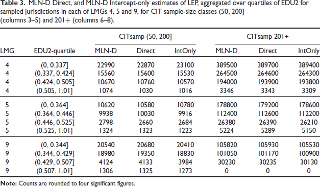
MLN-D Direct, and MLN-D Intercept-only estimates of LEP, aggregated over quartiles of EDU2 for sampled jurisdictions in each of LMGs 4,5 and 9, for CIT sample-size classes (50,200] (columns 3-5) and 20I+ (columns 6-8).
MLN-D Direct, and MLN-D Intercept-only estimates of LEP, aggregated over quartiles of EDU2 for sampled jurisdictions in each of LMGs 4,5 and 9, for CIT sample-size classes (50,200] (columns 3-5) and 20I+ (columns 6-8).
Although the covariates used in the MLN-D and MLN-F models are undoubtedly weak, likelihood analysis shows them to be highly significant in large LMGs. Supplement Tables S2 and S3 show the aggregated estimates by CIT sample-size category for the intercept-only MLN-D model. These tables do not show the aggregated MLN-D model predictions with covariates to be generally closer to the aggregated direct predictions than the intercept-only MLN-D predictions.
However, direct and MLN-D and intercept-only MLN-D estimates can also be aggregated over population subgroups defined by the covariates used in the models. The single covariate appearing most prominently in the LEP and ILL models is EDU2, the jurisdiction-level fraction of voting-age persons with no college education. Indeed, EDU2 is a covariate in each of the MLN-D models fitted to LEP and ILL outcomes in LMGs 4, 5 and 9. We next aggregated the estimates over all jurisdictions falling in each of four quartile intervals for EDU2 computed for the sampled jurisdictions for each of LMGs 4, 5 and 9 (not shown). Again for these aggregates, MLN-D with covariates agrees no better with the direct estimates than MLN-D fitted intercept-only. The reason for this is that the covariates in MLN-D dramatically improve the agreement of aggregated predictions with the Direct estimates in the size-classes (50,200] and 201+ where the great bulk of the LEP population (> 90%, for all three LMGs) falls. Table 3 shows the aggregated estimates for the EDU2 quartile intervals within the CIT sample-size class (50,200] in columns 3-5 and within the CIT sample-size class (200, ∞) in columns 6-8. This comparison shows that EDU2 does clearly have the effect of bringing the aggregated estimates from the MLN-D models with covariates much closer to the aggregated direct estimates than those from the Intercept-only models. The full Table S4 with all CIT sample-size classes is Included in the Supplement.
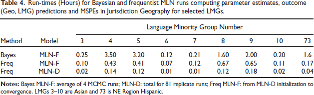
Run-times (Hours) for Bayesian and frequentist MLN runs computing parameter estimates, outcome (Geo, LMG) predictions and MSPEs in Jurisdiction Geography for selected LMGs.
Both frequentist and Bayesian analyses were used in producing estimates in the VRA Section 203(b) project, due to the special nature of the data. Differences in the numbers and sizes of jurisdictions among the different LMGs resulted in a wide variety of degrees of data-richness. The models that could be fitted in the LMGs, and the associated computational burdens, were sufficiently different that a flexible approach was necessary. This section summarizes comparisons made between Bayesian MLN-F and frequentist MLN-D and MLN-F methods, on 9 of the largest LMGs, numbered 3-10 and 73.
Frequentist estimates and predictions in the simpler MLN-D model were much easier to compute numerically than in the Bayesian MLN-F, so that MLE in MLN-D was the method of choice in all LMGs for exploratory data analyses with alternative model specifications. Table 4 shows runtimes for the two types of analysis, for LMGs 3-10 and 73 (Hispanic NE Region). The respective numbers of jurisdictions with ACS 2015-2019 sample in these LMGs were 989,3309, 4004, 742, 845, 3029, 3126, 1052 and 1045. The first row of Table 4 gives runtimes in hours for the average of four MCMC chains, although this advantages the Bayes methods. The third row displays the total run-time for the 81 replicate-weight frequentist MLN-D estimation and prediction runs. The second row gives the additional times for each LMG beyond the MLN-D initializations for a single fit using the original ACS weights.
The times in Table 4 to produce estimates in the MLN-F models are definitely faster for frequentist AGQ calculations than for Bayesian MCMC. However, Bayesian MCMC runs produce posterior variances as part of the same computation. With the frequentist estimates, MSPEs from parametric predictions based on model MLEs must be produced from 81 separate model-fitting calculations using SDR weight-replicates. The time required for 81 frequentist MLN-F calculations would not have been faster than the Bayesian MCMC calculations. The Bayesian approach was ultimately employed only for the most data-rich LMGs with Jurisdiction geography. In less data-rich LMGs, it was found that the MLN-F fitted models were not significantly different from the MLN-D fits, and the tremendously greater speed of MLN-D frequentist computations makes that method preferable on all but the largest LMGs.
All but one of the frequentist MLN-F fits in Table 4 used standard
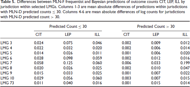
These purely computational considerations are relevant because the estimates from MLN-F models by Bayesian and frequentist methods were substantially the same. The estimates are not identical, typically differing only in the second or third decimal place, and in a very few cases in the first decimal place when estimated SEs are large (> 0.7). Table 5 quantifies the differences between frequentist and Bayesian MLN-F predictions and between frequentist MLN-F and MLN-D predictions, in (Geo, LMG) counts for outcomes CIT, LEP, and ILL The table quantifies the predicted differences separately for small and large counts. For jurisdictions where counts for an outcome are predicted (by frequentist MLN-D) to be ≤ 30, mean absolute differences of predicted counts are shown in the table’s first three columns. For jurisdictions with predicted outcome counts > 30, the table’s last three columns display mean absolute differences of (natural) logarithms of predicted counts. The discrepancies between MLN-F frequentist and Bayesian predictions are very small.
Differences between MLN-F frequentist and Bayesian predictions of outcome counts CIT, LEP, ILL by jurisdiction within selected LMGs. Columns I-3 are mean absolute differences of predictions within jurisdictions with MLN-D predicted counts ≤ 30. Columns 4-6 are mean absolute differences of log counts for jurisdictions with MLN-D predicted count > 30.
Differences between MLN-F frequentist and Bayesian predictions of outcome counts CIT, LEP, ILL by jurisdiction within selected LMGs. Columns I-3 are mean absolute differences of predictions within jurisdictions with MLN-D predicted counts ≤ 30. Columns 4-6 are mean absolute differences of log counts for jurisdictions with MLN-D predicted count > 30.
Estimated variances or MSPEs of the two types of model-based predictors are found to agree closely. An interesting pattern relates the SE differences to the size of the Bayes posterior SE for estimated LEP: when the Bayesian SEs are low (≤ 20), the frequentist SDR-based estimates are lower; for intermediate Bayes SEs (20-50), frequentist SEs are slightly lower or higher equally often; for medium-high Bayes SEs (50-300), frequentist SEs tend to be higher; and for higher Bayes SEs, the frequentist SEs are very slightly larger. This pattern for LEP-count SEs persists also with scaled-down ranges for ILL-count SEs. The estimated SEs track together fairly closely in all the LMGs investigated, with the largest but still tolerable differences seen in LMG 4, which is illustrated in Figure 3 for LEP.
The striking closeness of Bayesian to frequentist estimates and measures of uncertainty, despite their different origins, agrees with theory (Slud et al.)[32] (Section D.1). It is also practically important when considering a hybrid estimation strategy motivated by computational efficiency.
This paper has presented as an SAE problem an important, legally mandated, large-scale US statistical programme. Special features of the estimation task, described in the Introduction, have not previously appeared together in the SAE literature. These features led first of all to novel model choices. The nesting of the essential outcome subpopulations CIT, LEP and ILL within voting-age (Geo, LMG) domains strongly motivated models defined in a sequential conditional-probability form in 2011 and 2016 as well as in the recent 2021 VRA Section 203(b) programme cycle. Similar considerations had motivated the introduction of the continuation-ratio random effects model in a biomedical context with nested outcomes (Coull and Agresti)
Plots of estimated SEs by Frequentist SDR versus Bayesian MCMC for jurisdiction LEP counts in LMG4 for four ranges of successively larger SE estimates. Red lines are 45 ∘.
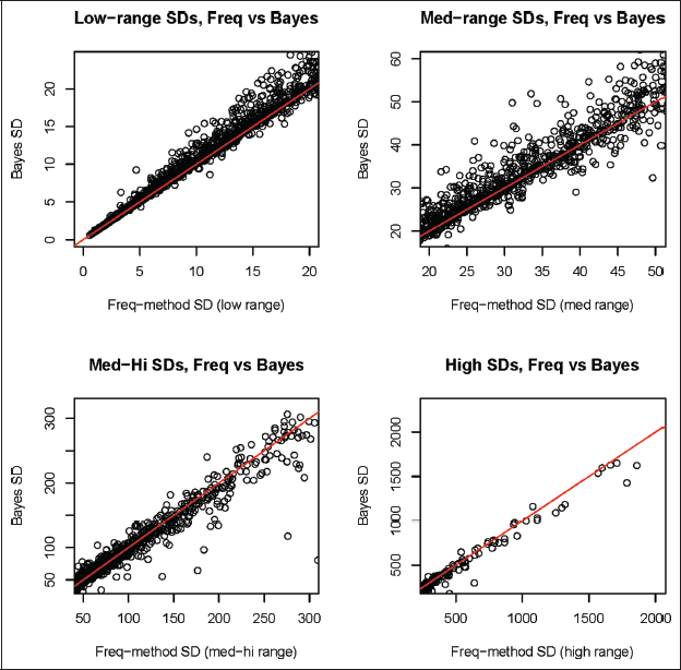
Plots of estimated SEs by Frequentist SDR versus Bayesian MCMC for jurisdiction LEP counts in LMG4 for four ranges of successively larger SE estimates. Red lines are 45 ∘.
Diagnostic assessments of the (Geo, LMG) model predictions were heavily driven by data imbalances, since the great majority of jurisdictions had tiny sample sizes while the bulk of population was concentrated in relatively few jurisdictions with large-sample sizes. Diagnostics showed that estimates from MLN-D and MLN-F successfully reduce MSPEs in the great majority of (Geo, LMG) domains; that in large LMGs the MLN models tend to over-predict LEP and ILL versus direct estimates in aggregated jurisdictions at tiny sample sizes, and then under-predict at middle sample sizes, with approximate equality at very high sample sizes; that covariates show little beneficial effect based on aggregated comparisons with direct estimates in large LMG tabulations of sample-size categories alone or covariate-quantile intervals alone; but that the covariates improve over intercept-only models in comparisons with direct estimates, when aggregated over sets of jurisdictions defined by covariate-quantile intervals and moderate-to-large (> 50) sample size.
The models presented in this paper have some limitations that were not addressed in the VRA project reports. These are of two broad types: the weakness of the available covariates, and model inadequacies due to the great majority of (Geo, LMG) domains in every LMG having very small size while the bulk of the population falls in a small number of large-sample domains.
The covariates available for our small area models were estimated from the same survey as the dependent variables. This necessitated estimation of covariates at higher levels of geographic aggregation and the removal of the sample overlap between the covariate and the dependent variables. Both of these steps can attenuate the relationship between the covariate and the dependent variable. Further, our covariates are ACS estimates subject to sampling error, but our model specifications ignore this error and treat covariates as if known precisely. It is known that such measurement errors can lead to noisier predictions and errors in estimated MSPEs (Ybarra and Lohr[36]; Bell et al.[4]). This imprecision in estimates makes our predictively weak covariates even weaker. The magnitude of this error will generally be larger for smaller geographic units, which have fewer sample observations.
Our diagnostics indicate that the MLN-D and MLN-F models tend on average to overestimate LEP and ILL counts on geographies with small-sample sizes and underestimate the counts in geographies with intermediate sample sizes. This seems to be due to a combination of the weakness of covariates and the practice of fitting a single model to all geographic units for each LMG regardless of sample size.
Future Directions
Various avenues for research might improve the current estimation methodology for future VRA Section 203(b) cycles. Some are specific improvements in computing or coordination of data sources, but most will involve new methodological work.
Administrative records may be an independent source of potentially stronger predictive covariates that avoid the pitfalls discussed above regarding measurement error and sample overlapping with the response. For the VRA application, challenges to overcome in using administrative records include: geocoding, lack of the necessary race/ethnicity information to compute the LMG in many of the sources, missing data, intricacies of the administrative records themselves, as well as difficulties in finding administrative-record fields predictive of the outcomes in (Geo, LMG) domains.
Another potential source from which to borrow strength in SAE models is past ACS five year direct estimates of outcome counts. The MLN-F model (2.5) could be extended to have random effects with a time dependence similar to a different multinomial logistic model (López-Vizcaíno et al.[19]. Such models could be generalized in a way that would also extend a recent temporal Binomial Logit-normal Model (Franco and Bell)[9] and could be estimated via Bayesian computation.
Future research in this area could fruitfully extend MLN models to account for covariate measurement error. Bayesian analysis of such models should be feasible using Stan (Stan Development Team)[33]. New research is also needed on ways to capture the effect of the survey design on the sample size for multinomial response data. The VRA covariates currently come from survey aggregates, and tiny geographic domains will have the most troublesome covariate errors-in-variables, diluting the effect of covariate-based prediction in those domains. This is a reason to fit models in the future with simple GVFs in which variances are scaled by sample size, as was done by Malec et al.[20]; Joyce et al.[14, 15] and in SAIPE (Bell et al.)[3]. A proposed method of defining multinomial effective sample size (McAllister and Iannelli)[22] was used in SAE (Maples)[21], but a more comprehensive study is needed.
Supplemental Material
Supplemental material for this article is available online.
Supplemental Material for Small area estimates for Voting Rights Act Section 203(b) coverage determinations by Eric Slud, Carolina Franco and Adam Hall, in Calcutta Statistical Association Bulletin
Footnotes
Acknowledgements
This paper is released to inform interested parties of research and to encourage discussion. The views expressed are those of the authors and not necessarily of the US Census Bureau. This research was performed under DMS project number 7510051. The statistics were released under DRB Clearance number CBDRB-FY23-CSRM001-0001.
Declaration of Conflicting Interests
The authors declared no potential conflicts of interest with respect to the research, authorship and/or publication of this article.
Funding
The authors received no financial support for the research, authorship and/or publication of this article.
References
Supplementary Material
Please find the following supplemental material available below.
For Open Access articles published under a Creative Commons License, all supplemental material carries the same license as the article it is associated with.
For non-Open Access articles published, all supplemental material carries a non-exclusive license, and permission requests for re-use of supplemental material or any part of supplemental material shall be sent directly to the copyright owner as specified in the copyright notice associated with the article.