Sage Journals: Discover world-class research

Abstract

Objective:

While risk factors for depression are increasingly known, there is no widely utilised depression risk index. Our objective was to develop a method for a flexible, modular, Risk Index for Depression using structural equation models of key determinants identified from previous published research that blended machine-learning with traditional statistical techniques.

Methods:

Demographic, clinical and laboratory variables from the National Health and Nutrition Examination Study (2009–2010, N = 5546) were utilised. Data were split 50:50 into training:validation datasets. Generalised structural equation models, using logistic regression, were developed with a binary outcome depression measure (Patient Health Questionnaire-9 score ⩾ 10) and previously identified determinants of depression: demographics, lifestyle-environs, diet, biomarkers and somatic symptoms. Indicative goodness-of-fit statistics and Areas Under the Receiver Operator Characteristic Curves were calculated and probit regression checked model consistency.

Results:

The generalised structural equation model was built from a systematic process. Relative importance of the depression determinants were diet (odds ratio: 4.09; 95% confidence interval: [2.01, 8.35]), lifestyle-environs (odds ratio: 2.15; 95% CI: [1.57, 2.94]), somatic symptoms (odds ratio: 2.10; 95% CI: [1.58, 2.80]), demographics (odds ratio:1.46; 95% CI: [0.72, 2.95]) and biomarkers (odds ratio:1.39; 95% CI: [1.00, 1.93]). The relationships between demographics and lifestyle-environs and depression indicated a potential indirect path via somatic symptoms and biomarkers. The path from diet was direct to depression. The Areas under the Receiver Operator Characteristic Curves were good (logistic:training = 0.850, validation = 0.813; probit:training = 0.849, validation = 0.809).

Conclusion:

The novel Risk Index for Depression modular methodology developed has the flexibility to add/remove direct/indirect risk determinants paths to depression using a structural equation model on datasets that take account of a wide range of known risks. Risk Index for Depression shows promise for future clinical use by providing indications of main determinant(s) associated with a patient’s predisposition to depression and has the ability to be translated for the development of risk indices for other affective disorders

Keywords

Depression psychiatry index structural equation modelling machine-learning

Introduction

With approximately 300 million cases estimated worldwide in 2010 (Ferrari et al., 2013), depression is a global health concern and is the second leading cause of years lived with a disability (Whiteford et al., 2013). Depression is associated with debilitating symptoms that not only affect the individual, but their family and community, and is expected to be the number 1 health concern in both developed and developing nations by 2020 (Lim et al., 2013). As exists for other well-known global health concerns, such as diabetes and cardiovascular disease, the development of a risk index to estimate individuals’ risk for depression would have overt benefits. However, the development of such a risk index requires a systematic and defensible methodological approach based on sound research.

A number of health risk indices currently available have primarily drawn on traditional statistical techniques for their development. For example, the Framingham Risk Score (FRS) was developed to measure the 10-year risk of cardiovascular disease (Dawber and Kannel, 1966) and utilised a logistic regression model for conditional risk using Walker-Duncan estimation, and updated to use Cox proportional-hazards regression in order to produce sex-specific prediction functions for assessing risk (D’Agostino et al., 2008). The Reynolds Risk Score was developed as an alternative to the FRS for cardiovascular risk assessment (Ridker et al., 2007) and used a mix of Cox proportional-hazards models, stepwise selection procedures and multiple additive regression trees (MART) to derive a set of models.

The Postoperative Vomiting score (Apfel et al., 1999) split data into approximately equal random training and validation sets. Binary logistic regression was run to develop the risk score on the training set and the models were validated using the validation dataset with the original coefficients. The Area under the Receiver Operation Characteristic (ROC) Curve (AUC) was used to assess the performance of the models.

The late-life dementia index was developed with the objective of accurately stratifying older adults into low-, moderate- or high-risk groups for developing dementia within 6 years and used logistic regression for its development (Barnes et al., 2009). The ROC curve was used to assess discrimination and for calibration purposes. A bipolar disorder risk of attempting suicide score was developed by a group based in Thailand (Ruengorn et al., 2012) using logistic regression to finalise the set of risk factors and developed a weighted total score split into low, moderate and high. The Chicago Adolescent Depression Risk Assessment used the boosted classification and regression trees machine-learning (ML) technique to develop a prediction index (Van Voorhees et al., 2008). Data were split into 60% training and 40% test, with the validity of the model being based on the sensitivity and specificity of the prediction model based with an optimal cut-off on the ROC curve.

Many of the current health risk indices implemented the approach of randomly splitting the data into training and validation or test sets and applying traditional statistical techniques to develop the indices. However, none have blended big data ML algorithms with traditional statistical techniques for the variable selection process in order to develop sets of domains, and establish their relative importance weightings for depression. This approach would enable a flexible, ‘modular’ aspect to the index, where determinants can be added/removed to a structural equation model (SEM) to estimate their simultaneous impact on the risk for depression.

Blending ML with traditional statistical techniques

The blending of unconstrained ML with constrained traditional statistical techniques in mental health research has considerable potential. ML algorithms have been implements for a pilot study into identifying risk of suicidality among patients with mood disorders (Passos et al., 2016). We have previously developed and applied a hybrid methodology that combined ML algorithms with traditional statistical modelling for variable selection, to detect key biomarkers associated with depression (Dipnall et al., 2016a). A blend of ML unsupervised self-organised mapping (SOM) and supervised boosted regression algorithms with logistic regression has been used to create, describe and validate depression clusters based on lifestyle-environs (Dipnall et al., 2017) and somatic symptoms (Dipnall et al., 2016b). These techniques have the benefits of achieving deep exploration of heterogeneous data to uncover the key relationships with depression.

This research builds upon our previously developed blended models that identified five domains of risk factors, which we call ‘determinants’, from systematic variable selection strategies that blended data mining with ML algorithms with traditional statistical techniques. The use of classes of risk factors in the construction of a risk index is novel. This study aims to develop a generalised structural equation model (GSEM) that utilises five identified previously published determinants of depression to establish their relative importance and test a theoretical Risk Index for Depression (RID) model. Each determinant will be constructed from a separate SEM. The GSEM will compute a (RID), measured on a scale of 0–100. The five depression determinants are represented as four separate formative depression models (demographics, lifestyle-environs, biomarkers and somatic symptoms) and a reflective diet depression model. Each determinant represents the probability of having depressive symptoms, based on the previous models derived.

The flexible approach allows further determinants to be added to the model without impacting on the methodology. Many known depression risk factors are not available in the dataset used in this study (e.g. stressful events), but our modular methodology allows additional determinants to be added from future datasets that possess data on these variables. This methodology also enables the relative strength of each determinant of depression to be established.

The theoretical RID model

The GSEM RID framework is represented in Figure 1. Prior research identified the risk factors associated with each determinant. It is anticipated that the probability of depression associated with all five determinants will model a path to the outcome of depression. However, for the first time, it is anticipated potential indirect paths exist from the probability of depression associated with demographics, lifestyle and diet through the impact these have on the probability of depression due to biomarkers and somatic symptoms. Indicative mediation effects using cross-sectional data have been used in other studies relating to depression such as to examine depression severity and associated risk factors for survivors of the 2008 Wenchuan earthquake in China (Xu et al., 2013) and to explore the specific indirect effects influencing the association between sex and established depression subtypes (Rodgers et al., 2016). An individual’s demographics can impact on their biomarkers (Van Spil et al., 2012) so it is conceivable this affects their probability of being depressed. Research has indicated positive associations between lifestyle factors and a depression risk (e.g. exercise has been shown to influence brain health, plasticity and depression risk, Jacka et al., 2011; Thomson et al., 2015; Van Praag et al., 2005), as has diet (Dipnall et al., 2015). Reduced blood flow and metabolism has also been associated in patients with bipolar disorder and depression (Baxter et al., 1989). Lifestyle and diet have an impact on somatic symptoms (Janssens et al., 2014). For example, for Type 2 diabetes mellitus and metabolic syndrome, diet is an important element of the management of this disease (Salas-Salvadó et al., 2016).

Figure 1.

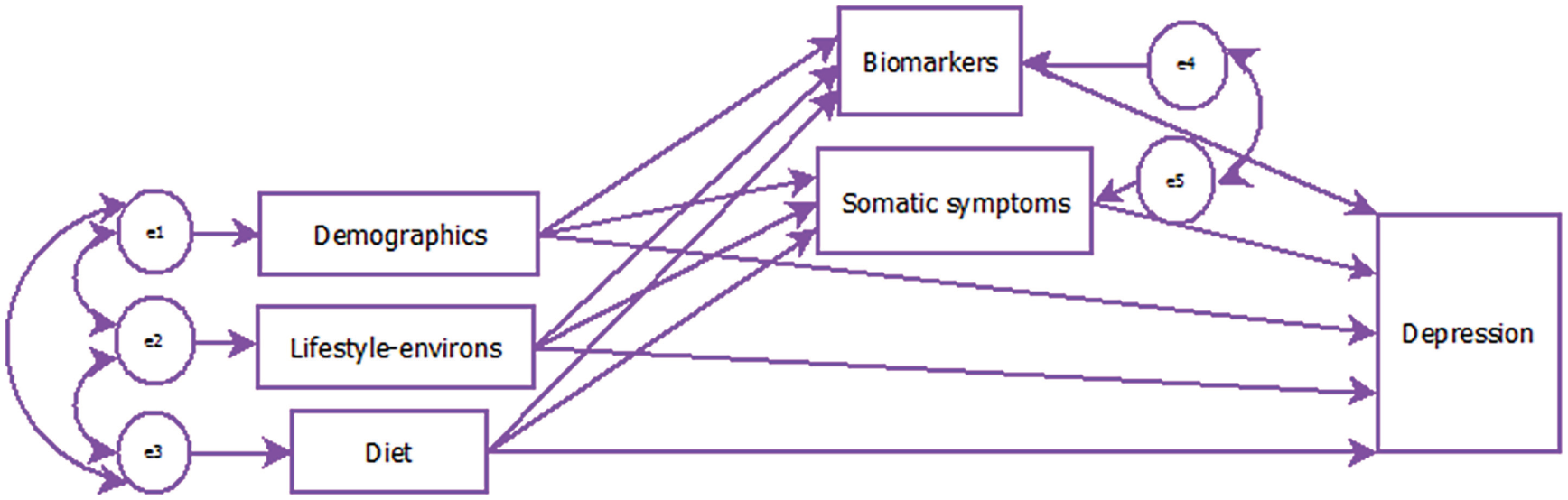
Generalised Structural Equation Model (GSEM) Risk Index for Depression (RID) path model.

The aim of this research was to develop a flexible, modular RID from epidemiological data using a systematic GSEM modelling approach building on previously published work.

Methods

National Health and Nutrition Examination Survey study design and participants

Community-based data from the 2009–2010 National Health and Nutrition Examination Survey (NHANES) (2009–2010) (Centers for Disease Control and Prevention [CDC] National Center for Health Statistics [NCHS], 2013) were used for this cross-sectional study (N = 5546, age range 18–80 years). The NHANES applied a complex four-stage sampling methodology: counties, segments within counties, households within segments and individuals within households. Data were collected from 15 locations across 50 US states, with oversampling of subgroups of the population of particular public health interest, to increase the reliability and precision of population estimates (CDC NCHS, 2013).

Use of data from the NHANES 2009–2010 database is approved by the NCHS Research Ethics Review Board (Continuation of Protocol #2005-06).

Outcome measure

A self-reported Patient Health Questionnaire-9 (PHQ-9) (Kroenke and Spitzer, 2002) was used to assess depressive symptoms (‘depression’). This questionnaire consisted of nine items that were summed to form a total score, where a total score of 10 or more was considered moderately or severely depressed.

Statistical methodology

The five-stage statistical process performed for this research is outlined in Figure 2. The different GSEM models are indicated, where rectangles represent observed variables, the large circle represents the latent diet variable, and the small circles represent the measurement errors. STATA V14 was used in all statistical analyses.

Figure 2.

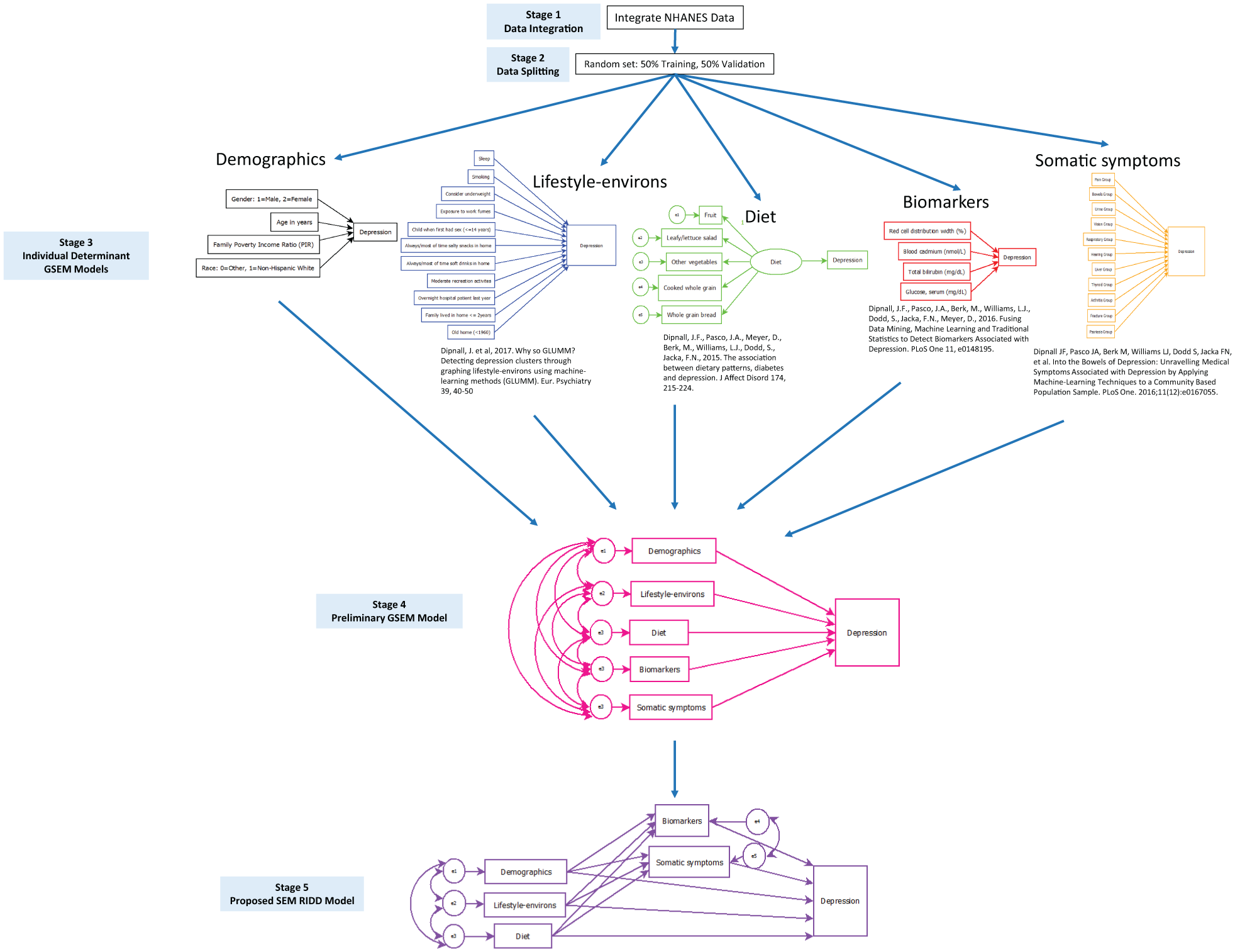
Five-stage methodology for the final generalised structural equation model (GSEM) Risk Index for Depression (RID) path model.

Stage 1 integrating NHANES data

Questionnaire and laboratory data were downloaded from the NHANES website and integrated using the Data Integration Protocol in Ten Steps (DIPIT) methodology (Dipnall et al., 2014).

Stage 2 data splitting

To help assess the quality of the predictive models, data were randomly split into two datasets. At each stage of the analysis, 50% of the data were used to formulate or train each of the models (training) and the remaining 50% were used to validate the training models. Training and validation datasets were checked for similarity on depression, age, gender and predictor variables.

The stages of the GSEM in Figure 1 were performed with depression as a binary outcome assuming a Bernoulli distribution and running logistic regression. All GSEM models took account of the complex sampling methodology of the NHANES data. A GSEM probit model was also run for the final-stage model with the binary depression dependent variable and assumed that the probability of a positive outcome was determined by the standard normal cumulative distribution function. This was performed to further validate the GSEM logistic model.

Stage 3 individual GSEM determinant models

At the first stage of the analysis, separate GSEM models were run for the demographics, diet, lifestyle-environs, biomarkers and somatic symptoms determinants (Culbertson, 1997; Dipnall et al., 2015, 2016a, 2016b, 2017; Mirowsky and Ross, 1992; Riolo et al., 2005) (Figure 2). The variables used for the diet, lifestyle-environ, biomarkers and somatic symptoms determinant models were based on our previous research, which utilised big data mining and ML techniques applied to a greater number of possible risk factors. Formative path models were run for the demographics, lifestyle-environs, biomarkers and somatic symptoms determinants. A confirmatory factor analysis (CFA) was run for the diet determinant to afford a better measure of the latent variable (Diet), by isolating the shared variance of the five food frequency items in the latent variable from their unique variance. Predicted probabilities of depression were generated from each of the five determinant models for both the training and validation datasets. These probabilities were then converted to logits order to ensure that a linear combination of determinants could be applied to obtain the logit for depression for the final RID model. Similarly, probit conversions were applied to obtain the final probit depression model.

Demographics determinant of depression

The demographics determinant model was a GSEM recursive model (i.e. no feedback loops or correlated errors). The following socio-demographic predictors of depression were isolated from the NHANES questionnaire data: gender (male, female), age in years, family poverty income ratio (PIR) and race (non-Hispanic white, other), as shown in the model in Stage 2 of Figure 2. Age-squared was included in the demographic determinant GSEM path model to ensure a better fit.

Diet determinant of depression

The primary dietary data were originally derived from a 24-hour dietary recall interview for NHANES participants, conducted in person by trained dietary interviewers (Thompson and Byers, 1994). A second dietary interview for all participants who complete the in-person recall was collected by telephone approximately 3–10 days later, yielding information on the regular consumption of the five key dietary components of fruit, leafy/lettuce salad, other vegetables, cooked whole grain and whole grain bread.

Previous exploratory factor analysis (EFA) identified five healthy dietary components to form the latent Diet factor, which was inversely associated with depression (Dipnall et al., 2015) (Diet model, Stage 2, Figure 2). The current study used CFA to obtain a measurement model for this dietary factor. The circle labelled Diet on the diagram was the unobserved, latent variable and the circles attached to each of the five observed dietary components are their unique measurement errors. The weight for the observed fruit component was fixed to 1 in order to make estimation possible. The concept of a latent diet factor has previously been applied to dietary data from the Reasons for Geographic and Racial Differences in Stroke (REGARDS) study (Judd et al., 2015).

Lifestyle-environs determinant of depression

Eleven key lifestyle-environs variables used for this study were identified in our previous research from 96 original NHANES lifestyle-environs self-report variables that covered a broad cross-section of categories: work status, physical activity, healthcare usage, sleep, smoking, blood donation, sexual activity, drug usage, diet, grocery shopping habits, meal habits, pesticide usage, air quality and home attributes (Dipnall et al., 2017). Unsupervised and supervised ML techniques were previously used to identify the lifestyle-environs risk factors associated with depression. The well-established risk factors for depression, including sleep problems (Berk, 2009), unhealthy snacks in the home (Camilleri et al., 2014) and lack of physical recreational activity (Jacka et al., 2011), were identified. The potential risk factors of exposure to fumes at work for depression were included in this study, being consistent with previous research relating to links to depression (Nel, 2005). The links to depression relating to the age of the home and short period of time residing in the home (⩽2 years) are thought to be related to instability in home and/or working life (Weissman and Paykel, 1972) and potentially lower monthly family income. The inclusion of sexual activity at an early age (i.e. <14 years) as a potential risk factor for depression was consistent with research indicating an association between adolescent sexual activity and an increased likelihood of depression (Hallfors et al., 2005). Smoking status (0 = never smoked, 1 = smoker) was also included in the lifestyle-environs determinant model as research has shown that cigarette smoking has been associated with depression (Boden et al., 2010). The lifestyle-environs predictors were initially compiled using a recursive SEM path model where each of the 11 observed variables had a direct path to depression (Lifestyle-environs model, Stage 2, Figure 2).

Biomarkers determinant of depression

We previously applied a blend of supervised ML boosted regression algorithm with traditional binary logistic regression to 67 original NHANES blood and urine samples to identify four key biomarkers most strongly associated with depression (Dipnall et al., 2016a): red cell distribution width (%), blood cadmium (nmol/L) and total bilirubin (mg/dL), and serum glucose (mg/dL). The original laboratory samples were collected in the NHANES Mobile Examination Center (MEC) and shipped weekly for laboratory analyses. Specific laboratory techniques for each test are available from the NHANES Laboratory Procedures Manual (CDC, 2009–2010). For this study, the biomarker predictors were initially compiled using a recursive SEM path model where each of the four observed variables had a direct path to depression (Biomarker model, Stage 3, Figure 2).

Somatic symptoms determinant of depression

There is a high level of comorbidity between somatic symptoms and depression (Kapfhammer, 2006). Using 68 self-reported medical symptom questions from the NHANES questionnaire data, and applying a blend of unsupervised SOM, hierarchical clustering and supervised ML boosted regression algorithms with traditional logistic regression, we previously identified 11 key somatic symptom categories of pain, bowels, urine, vision, respiratory, hearing, liver, thyroid, arthritis, fracture and psoriasis as most strongly associated with depression (Dipnall et al., 2016b). The 11 observed somatic symptom variables in this study were compiled using a recursive SEM path model representing a direct association with depression (Somatic symptom model, Stage 2, Figure 2).

Stage 4 direct GSEM path model

The Stage 4 preliminary GSEM path model incorporated all the determinant logits generated from Stage 3 as observed exogenous variables (i.e. determined outside the current model, represented by the rectangles, Stage 4 model, Figure 2). Correlations between the errors of all of the observed determinants of depression were included (i.e. curved arrows). All paths at Stage 4 were direct to the depression logit outcome binary variable. Odds ratios (ORs) and 95% confidence intervals (95% CI) for each determinant from this model represented its relative importance association with depression.

Stage 5 GSEM RID model

The Stage 4 GSEM model was modified to define the biomarker and symptom determinant models as observed endogenous variables (i.e. rectangles, Figure 1). The correlation between the errors of biomarkers and somatic symptoms determinant logits were included. The demographics, lifestyle-environs and determinant logits had direct paths to depression, as well as indirect paths to depression through their impact on biomarkers and somatic symptoms determinant logits. Thus, all possible relationships among the risk variables with depression were able to be explored (i.e. direct, indirect and total relationships). Predicted probabilities for total depression risk were generated from the final model for both the training and validation datasets

Fit indices

The nature of the NHANES data, with its complex survey structure, meant that the standard absolute and comparative fit indices (e.g. model χ², root mean square error of approximation, goodness-of-fit (GOF) statistic, adjusted GOF statistic, normed-fit index and comparative fit index) could not be produced. The use of the actual Akaike information Criterion, Bayesian information criterion (BIC) and Sample-Size Adjusted BIC was not possible for the same reason.

The dilemma of finding appropriate fit statistics was resolved by using the Hosmer and Lemeshow GOF F-test (Hosmer and Lemeshow, 1980) only for the Stage 4 path model as the Stage 3 models did not control for potential demographic confounders. A model was deemed a good fit if the p-value for this statistic was not significant (p > 0.05, preferably p > 0.10). In addition, consistent with other health indices, the AUC (i.e. C-Statistic) was also used as an indication of fit for the training and validation models at every stage of the analysis (Linden, 2006). This is a standard measure of the predictive accuracy of a binary logistic regression model to determine how good the model will be at distinguishing (or ‘discriminating’) between those with and without depression, and has been used to evaluate other health risk index models. This measure takes values from 0 to 1, where a value of above 0.7 is considered acceptable.

Results

Stage 2 data splitting

The data were randomly split, with 50% for training (n = 2773) and 50% for validation (n = 2773), and the split was found to be approximately consistent across the binary depression outcome variable and observed explanatory variables (Table 1).

Table 1.

Unweighted and estimated mix of training compared to validation datasets.

	Unweighted		Estimated^a
	Training	Validation	Training	Validation
	n = 2773	n = 2773	n = 2310	n = 2344
Depressed	258 (9.3%)	265 (9.6%)	226 (7.8%)	250 (8.3%)
Demographics
Gender
Male	1308 (50.4%)	1296 (49.3%)	1095 (51.6%)	1097 (49.3%)
Female	1289 (49.6%)	1334 (50.7%)	1076 (48.4%)	1132 (50.7%)
Race
Other	1214 (55.9%)	1217 (54.6%)	1214 (32.6%)	1217 (31.9%)
Non-Hispanic White	957 (44.1%)	1012 (45.4%)	957 (67.4%)	1012 (68.1%)
Age (years), mean (SD/SE)^b	42.51 (14.98)	42.74 (15.07)	42.21 (0.38)	42.67 (0.42)
Family Poverty Income Ratio (PIR), mean (SD/SE)^b	2.48 (1.64)	2.44 (1.62)	3.05 (0.05)	3.02 (0.05)
Lifestyle
Trouble sleeping/sleep disorder	712 (25.7%)	722 (26.0%)	566 (25.3%)	593 (26.9%)
Ever had work exposure to other fumes	794 (31.8%)	847 (33.7%)	721 (32.8%)	777 (33.2%)
Consider weight – underweight	147 (5.3%)	118 (4.3%)	116 (4.6%)	91 (3.2%)
Age when first had sex – Child (⩽14 years)	361 (16.9%)	384 (17.9%)	361 (14.3%)	304 (14.6%)
Salty snacks in home Always/Most of time	1526 (55.5%)	1516 (55.2%)	1287 (61.5%)	1286 (60.6%)
Soft drinks in home Always/Most of time	1374 (50.0%)	1414 (51.5%)	1175 (51.2%)	1227 (52.1%)
Moderate recreational activity	1068 (38.5%)	1090 (39.3%)	921 (47.4%)	943 (45.5%)
Overnight hospital patient in last year	364 (13.1%)	356 (12.8%)	256 (9.2%)	265 (9.5%)
Family lived in home 2 years or less	794 (28.9%)	778 (28.2%)	766 (29.9%)	743 (28.9%)
Old home (<1960)	820 (37.5%)	800 (36.7%)	644 (33.0%)	648 (32.9%)
Never smoked	1153 (56.0%)	1108 (53.0%)	1153 (56.8%)	1108 (54.2%)
Diet
How often eat fruit? mean (SD/SE)^b	0.70 (0.02)	0.72 (0.02)	0.74 (0.03)	0.75 (0.02)
How often eat leafy/lettuce salad? mean (SD/SE)^b	0.38 (0.01)	0.36 (0.01)	0.41 (0.01)	0.39 (0.02)
How often eat other vegetables? mean (SD/SE)^b	0.63 (0.01)	0.63 (0.01)	0.70 (0.02)	0.71 (0.02)
How often eat cooked whole grains? mean (SD/SE)^b	0.09 (0.01)	0.09 (0.01)	0.08 (0.01)	0.09 (0.01)
How often eat whole grain bread? mean (SD/SE)^b	0.46 (0.01)	0.46 (0.01)	0.48 (0.01)	0.49 (0.02)
Biomarkers
Red cell distribution width (%), mean (SD/SE)^b	12.91 (1.25)	12.92 (1.36)	12.69 (0.05)	12.76 (0.03)
Blood cadmium (nmol/L), mean (SD/SE)^b	4.40 (4.56)	4.63 (5.12)	4.18 (0.14)	4.44 (0.13)
Total bilirubin (mg/dL), mean (SD/SE)^b	0.76 (0.32)	0.76 (0.28)	0.77 (0.01)	0.77 (0.01)
Glucose, serum (mg/dL), mean (SD/SE)^b	100.91 (0.69)	100.57 (0.70)	96.79 (0.76)	96.21 (0.81)
Somatic symptoms
Pain Group	660 (30.1%)	689 (31.3%)	660 (30.2%)	689 (30.8%)
Bowels Group	1195 (45.4%)	1221 (46.7%)	963 (40.5%)	997 (42.2%)
Urine Group	981 (37.2%)	1009 (38.5%)	730 (30.2%)	774 (32.8%)
Vision Group	491 (17.7%)	471 (17.0%)	386 (14.3%)	383 (12.9%)
Respiratory Group	900 (32.5%)	899 (32.4%)	784 (33.7%)	794 (32.0%)
Hearing Group	591 (21.3%)	573 (20.7%)	406 (18.5%)	390 (16.4%)
Liver Group	91 (3.4%)	81 (3.1%)	80 (3.3%)	67 (2.3%)
Thyroid Group	239 (9.0%)	277 (10.5%)	162 (7.7%)	185 (9.4%)
Arthritis Group	702 (26.5%)	753 (28.7%)	454 (19.7%)	504 (21.3%)
Fracture/Osteo Group	381 (14.4%)	368 (14.0%)	263 (13.0%)	266 (12.4%)
Psoriasis Group	79 (2.8%)	81 (2.9%)	68 (3.2%)	64 (2.8%)

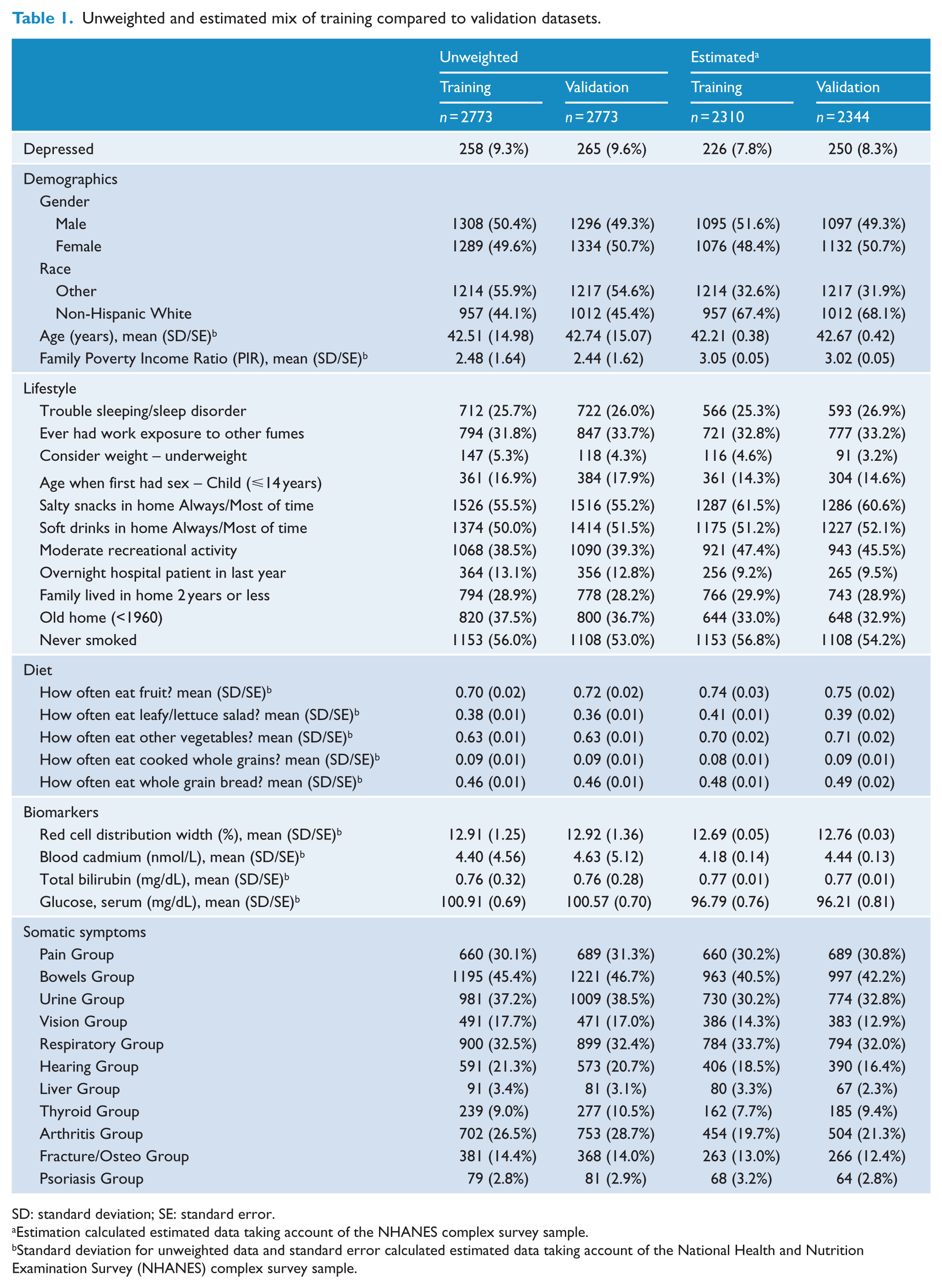
SD: standard deviation; SE: standard error.

Estimation calculated estimated data taking account of the NHANES complex survey sample.

Standard deviation for unweighted data and standard error calculated estimated data taking account of the National Health and Nutrition Examination Survey (NHANES) complex survey sample.

Stage 3 individual GSEM determinant models

The ROC analysis results for the individual depression determinant models are summarised in Table 2. The AUCs for the individual demographics, diet and biomarker determinants were all below 0.7. The AUCs were acceptable at above 0.7 for both the somatic symptoms (AUC = 0.741) and lifestyle-environs (AUC = 0.780) determinant models.

Table 2.

Stage 3 GSEM determinant models AUC results.

GSEM Logistic Regression Model	Training			Validation
	AUC	95% CI		AUC	95% CI
	AUC	Low	High	AUC	Low	High
Stage 3 Individual Determinant GSEM Models
Demographics = Pr(Depress-demo)	0.686	0.646	0.725	0.700	0.662	0.737
Lifestyle-environs = Pr(Depress-lifest)	0.780	0.740	0.821	0.738	0.692	0.783
Diet = Pr(Depress-diet)	0.688	0.650	0.725	0.664	0.625	0.703
Biomarkers = Pr(Depress-bio)	0.638	0.600	0.677	0.642	0.606	0.679
	0.741	0.705	0.777	0.747	0.713	0.782

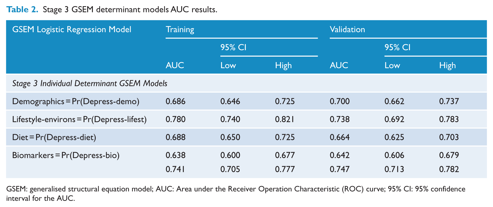
GSEM: generalised structural equation model; AUC: Area under the Receiver Operation Characteristic (ROC) curve; 95% CI: 95% confidence interval for the AUC.

Probabilities were generated from each determinant model and transformed into logits. In order to establish associations and check for multicollinearity, the correlations between the logit probabilities (logits) are presented (Table 3). With the exception of diet and somatic symptoms determinant logits, where there was no significant correlation (r = 0.030, p = 0.112), all pairs of determinant logits had very weak to weak but significant positive correlations with depression. This statistically justifies the inclusion of biomarkers and somatic symptoms as potential mediators for the demographics and lifestyle determinants in the final GSEM model at Stage 5 (Hayes, 2009). Although there was a significant correlation between the diet and biomarkers determinant logits, the strength of the correlation for these variables indicated virtually no linear relationship (r = 0.052, p = 0.007). These results indicated that mediation relationships between the diet logit determinant and both biomarkers and somatic symptoms logit determinants were unlikely.

Table 3.

Correlations of logits determinants.

Correlations (n = 2775)	Demographics	Lifestyle-environs	Diet	Biomarkers	Somatic Symptoms
Determinant	logit(Pr[Depress-demo])	logit(Pr[Depress-lifest])	logit(Pr[Depress-diet])	logit(Pr[Depress-bio])	logit(Pr[Depress-som])
logit(Pr[Depress-demo])	1.000
logit(Pr[Depress-lifest])	0.215***	1.000
logit(Pr[Depress-diet])	0.120***	0.141***	1.000
logit(Pr[Depress-bio])	0.253***	0.254***	0.052**	1.000
logit(Pr[Depress-som])	0.191***	0.290***	0.030	0.215***	1.000

***

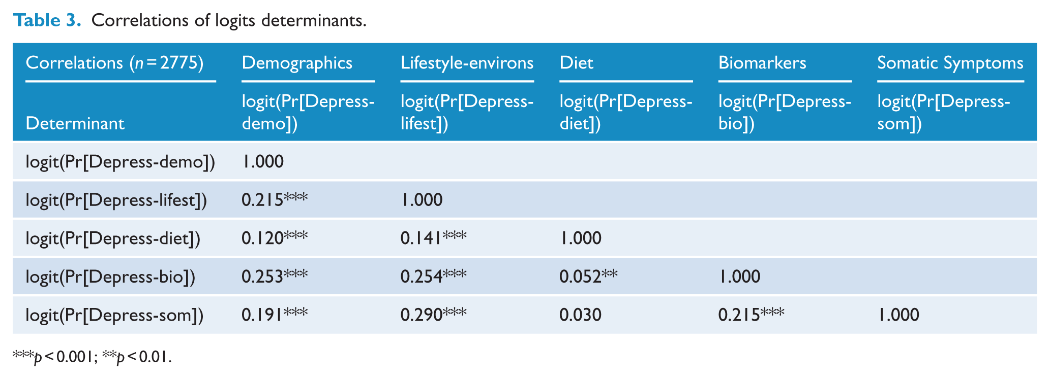
p < 0.001; **p < 0.01.

Stage 4 direct GSEM path model

The results from the direct GSEM path model is presented in Figure 3. The ORs for the direct paths from each logit determinant to depression indicated the relative importance of each determinant on the depression logit. Of highest rank was the diet determinant, with OR 4.09 (95% CI: [2.01, 8.35]), then lifestyle-environs (OR 2.15; 95% CI: [1.57, 2.94]), somatic symptoms (OR 2.10; 95% CI: [1.58, 2.80]), demographics (OR 1.46; 95% CI: [0.72, 2.95]) and lastly biomarkers (OR 1.39; 95% CI: [1.00, 1.93]). All relationships were positive due to the determinants representing the probability of being depressed, generated from Stage 3 models. The direct path from the demographics logit to depression was not significant (p = 0.276) and the direct path from the biomarker logit to depression was of borderline significance (p = 0.052).

Figure 3.

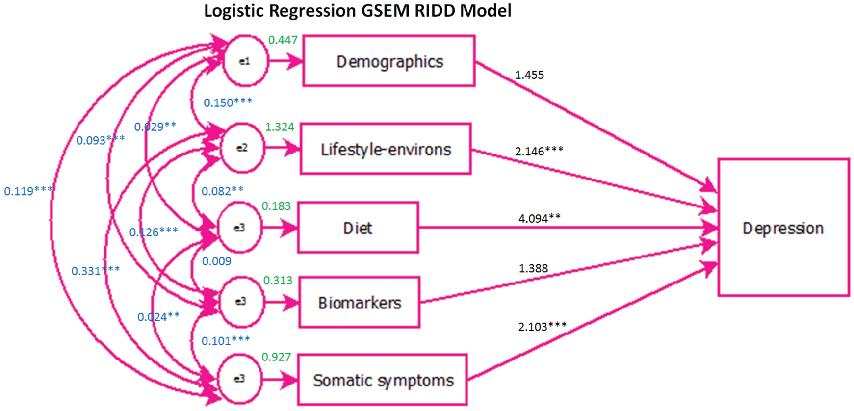
Stage 4 direct generalised structural equation model (GSEM) path model.

The ROC analysis results for the Stage 4 preliminary GSEM path model were very good (AUC training = 0.854, validation = 0.827). However, the GOF test was significant (p = 0.001) which suggested that the direct model was not a good fit.

Stage 5 GSEM RID model

The proposed Stage 5 GSEM RID path model was fitted for both logistic regression and probit regression to test consistency. The direct path from the demographics logit determinant to depression was removed, as this path was found to be not significant for both the logistic regression (p = 0.276) and probit regression (p = 0.219) GSEM path models. Thus, the probability of depression due to demographics potentially only affected depression indirectly through its impact on the probability of depression due to biomarkers and somatic symptoms. In addition, the indirect paths from the probability of depression due to diet to the probability of depression due to biomarkers (logistic regression: p = 0.845; probit regression: p = 0.981) and somatic symptoms (logistic regression: p = 0.933; probit regression: p = 0.872) were removed from the model because they were not significant. This was consistent with the low correlation between the diet and biomarkers and somatic symptom determinant logit (Table 3).

The revised and final GSEM RID logit path model is presented in Figure 4. All correlations and direct and possible indirect paths to the depression logit were significant at α = 0.05. The logits from the biomarker and somatic symptom determinant models were kept as observed endogenous variables. The correlation between the errors of biomarkers and somatic symptoms logit determinants were maintained as they were found to be significant (logistic regression: p = 0.010; probit regression: p = 0.011). Direct paths to depression were maintained for the lifestyle-environs and diet determinant logits. The final probit model is also shown in Figure 4.

Figure 4.

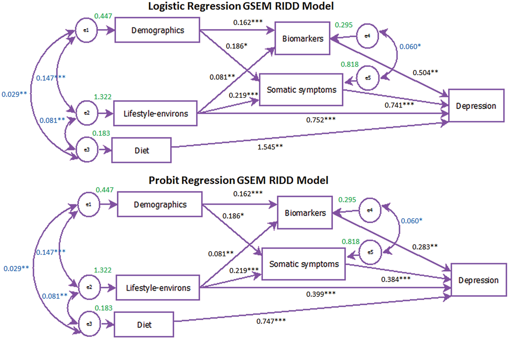
Stage 5 Final Generalised Structural Equation Model (GSEM) Risk Index for Depression (RID) path models for logistic and probit regression.

In general, the AUC results were consistent for both the logistic and probit models (Logistic: training = 0.850, validation = 0.813; Probit: training = 0.849, validation = 0.809). Even though there was a reduction in the AUC from Stage 4 to Stage 5, the difference was not significant and all paths in the final model were significant. The predicted probabilities of depression from this GSEM ranged from 0 to 1 and were consistent across logistic and probit regressions.

Discussion

In previous research, models for determinants (including the individual factors) of depression were developed using ML methods. In this study, SEM combines these determinants into a multi-faceted prediction for the probability of depression. To our knowledge, this is the first study that has blended ML with traditional statistical techniques in this fashion to formulate a RID. The five identified determinants on their own are not enough to provide a holistic prediction of depression as other known risks are not available in this dataset, but together they formed a consistent model for RID, with significant direct and indirect pathing and a good AUC. The modular structure of the method allows future research to strengthen the RID by including other known or potential risk factors for depression not available in the NHANES data. For this study, the indicative importance ranking of the individual determinants of depression, where diet was ranked first, followed by lifestyle-environs, somatic symptoms, demographics and biomarkers, represents new research findings. However, these rankings may alter once other determinants are added to the GSEM. The identification of a patient’s potential risk of depression would greatly benefit from the addition of other potential determinants (e.g. personality traits) to the model; this would allow for a more holistic RID that could be used as tool for clinicians to identify high-risk groups and to deliver targeted prevention programmes. The RID can further inform the Royal Australian and New Zealand College of Psychiatrists clinical practice guidelines for mood disorders (Mood Disorders CPG) for practitioners of mental healthcare (Malhi et al., 2015).

Our results indicate that only diet has a direct association with depression. The diet determinant comprised fibre-rich foods such as leafy green salad, vegetables and whole grains. Such dietary components have been consistently associated with a reduced risk for depression. Moreover, dietary fibre appears central to gut health, which has recently been a key focus of depression research (Dash et al., 2015). We have very recently identified bowel symptoms as the most prominent somatic symptom associated with depression (Dipnall et al. 2016b) and our findings provide further support for diet as a key modifiable factor in depression risk. The RID could be used with longitudinal data to determine possible indirect paths from diet to depression.

The lifestyle-environs determinant was found to have both a direct association with depression and also an indirect association via symptoms and biomarkers. Lifestyle factors, such as sleep problems (Berk, 2009), tobacco smoking (Taylor et al., 2014), snacking behaviour and exercise activity (Pasco et al., 2011), have all been found to be associated with individuals’ physical and mental health.

This study found that the demographic determinant was related to depression only indirectly via symptoms and biomarkers. Differences in biomarkers and somatic symptoms according to age, gender, race and socio-economic status are well established. For example, increasing age is associated with a higher likelihood of chronic disorders. The direct path from biomarkers and somatic symptoms to depression in the RID model confirmed prior research identifying that depressive symptoms are often elevated in people with medical symptoms (Olver and Hopwood, 2012).

Alternative models to those proposed here are possible. While research has indicated there are possible bidirectional relationships of some of the key risk determinants with depression (e.g. diet), due to the nature of the cross-sectional data, this study focused on the outcome being the probability of depression. With further development of the RID, it is anticipated the future use of this index could focus on identifying risk determinants to inform prevent strategies for depression onset.

Strengths and limitations

A key limitation of our study is the cross-sectional nature of the NHANES data, restricting the ability to infer causality and mediation paths, so the RID requires further validation in longitudinal datasets. Data on many important and known risk factors were not available in this dataset. However, this methodology has the potential to be used in future datasets with a wider range of variables. The use of this large community-based survey dataset has the advantage of being representative of the large US population sampled during 2009 to 2010. The rigorous complex survey sampling methodology also ensured the data represent the relative characteristics of the civilian noninstitutionalised US population.

Due to the nature of the complex survey data structure, conventional fit statistics for the SEMs were not available. However, the AUC for both training and validation and across two types of regression models (logistic and probit) was utilised.

The PHQ-9 instrument is limited by being a self-report measure of depressive symptoms rather than a clinical diagnosis of depression, thereby potentially biasing case ascertainment (Kroenke et al., 2001; Kroenke and Spitzer, 2002). However, the NHANES study is considered representative of the US noninstitutionalised civilian population and has been used to produce health statistics for the United States and in many studies investigating depression (e.g. to examine the prevalence, treatment and control of depressive symptoms) (Shim et al., 2011).

The data were split into 50% training and 50% validation, ensuring that a reasonable proportion of those with depressive symptoms were included in each set. This allowed the GSEM models to be validated using a random portion of the NHANES data. However, the RID was not validated using a separate dataset but there is potential to apply this methodology to other data, including longitudinal data, for validation purposes.

Often, the limitations of SEM relate to sample size, which needs to be large enough to obtain stable estimates of the covariances/correlations. In general, a model requires at least 200 participants, and for a path model, the sample size should be at least 20 times larger than the number of estimated paths to ensure reliable results (Jeon, 2015). Even with the splitting of the data, the sample size for this study met the SEM requirements. It could be argued that a limitation is that the model may omit some variables that are of theoretical relevance. However, selection of the variables constituting the depression determinants for this research was based on our previous research, which utilised big data mining and ML techniques applied to a much larger number of possible risk factors. Last, this paper provides a modular methodology for the development of the risk index; the nature of the NHANES data, as previously outlined, limits the extent to which the results might represent a definitive and accurate summative risk profile for depression.

Conclusion

This study developed a flexible modular methodology for the development of a novel RID, measured on a scale of 0–100, with foundations for a future more complex SEM. The preliminary model used in this study was developed using complex cross-sectional survey data, based on previous research that utilised both ML and traditional statistical techniques to formulate the depression risk determinants. An indicative importance ranking of the individual determinants of depression was produced. From the NHANES data, diet was ranked first, then lifestyle-environs, somatic symptoms, demographics and biomarkers. Our preliminary results suggest that diet has a direct association with depression, but other lifestyle-environs and demographic factors appear to be associated indirectly with depression via somatic symptoms and biomarkers. However, further validation is required, including refinement by using datasets that include a wider range of variables. The RID has the potential to assist clinicians with the identification of people at risk of depression, and potentially other affective disorders, by prioritising risk determinants in support of targeted interventions.

Footnotes

Acknowledgements

The authors would like to thank the Editor and referees of this issue for their valuable and insightful comments and suggestions that have improved this paper. J.F.D. contributed equally to this work. J.F.D. is the primary author for this manuscript: performed the literature search; designed and performed the statistical methodology and analysis, interpretation of the statistical results; created the figures; prepared the tables; and wrote the initial manuscript. J.F.D., J.A.P., M.B., L.J.W., S.D., F.N.J. and D.M. were involved in the interpretation of data for the work and writing of the manuscript, approved the final version, and agreed to be accountable for all aspects of the work in ensuring that questions related to the accuracy or integrity of any part of the work are appropriately investigated and resolved.

Declaration of Conflicting Interests

J.F.D. has nothing to disclose. J.A.P. has nothing to disclose. M.B. reports personal fees from consultancy, personal fees from employment, grants from grants/grants pending, personal fees from payment for lectures, personal fees from royalties, outside the submitted work. S.D. has nothing to disclose. L.J.W. has nothing to disclose. F.N.J. has nothing to disclose. D.M. has nothing to disclose. J.F.D. has no conflicts of interest in relation to this manuscript. J.A.P. has recently received grant/research support from the National Health and Medical Research Council (NHMRC), BUPA Foundation, Amgen/GlaxoSmithKline/Osteoporosis Australia/Australian and New Zealand Bone and Mineral Society, Western Alliance, Barwon Health, Deakin University and the Geelong Community Foundation. M.B. has received grant/research support from the NIH, Cooperative Research Centre, Simons Autism Foundation, Cancer Council of Victoria, Stanley Medical Research Foundation, MBF, NHMRC, Beyond Blue, Rotary Health, Geelong Medical Research Foundation, Bristol Myers Squibb, Eli Lilly, Glaxo SmithKline, Meat and Livestock Board, Organon, Novartis, Mayne Pharma, Servier and Woolworths; has been a speaker for Astra Zeneca, Bristol Myers Squibb, Eli Lilly, Glaxo SmithKline, Janssen Cilag, Lundbeck, Merck, Pfizer, Sanofi-Synthelabo, Servier, Solvay and Wyeth; and served as a consultant to Allergan, Astra Zeneca, Bioadvantex, Bionomics, Collaborative Medicinal Development, Eli Lilly, Glaxo SmithKline, Janssen Cilag, Lundbeck Merck, Pfizer and Servier. M.B. is supported by a NHMRC Senior Principal Research Fellowship 1059660. L.J.W. has received grant/research support from Eli Lilly, Pfizer, The University of Melbourne, Deakin University and the NHMRC and is supported by a NHMRC Career Development Fellowship (1064272). S.D. has received grants/research support from the Stanley Medical Research Institute, NHMRC, Beyond Blue, ARHRF, Simons Foundation, Geelong Medical Research Foundation, Fondation FondaMental, Eli Lilly, Glaxo SmithKline, Organon, Mayne Pharma and Servier; speaker’s fees from Eli Lilly; advisory board fees from Eli Lilly and Novartis; and conference travel support from Servier. F.N.J. has received grant/research support from the Brain and Behaviour Research Institute, the National Health and Medical Research Council (NHMRC), Australian Rotary Health, the Geelong Medical Research Foundation, the Ian Potter Foundation, Eli Lilly, the Meat and Livestock Board and The University of Melbourne and has received speakers honoraria from Sanofi-Synthelabo, Janssen Cilag, Servier, Pfizer, Health Ed, Network Nutrition, Angelini Farmaceutica and Eli Lilly. She is supported by an NHMRC Career Development Fellowship (#1108125). D.M. has received grant/research support from the Australian research Council (ARC), Mental Illness Research Fund (MIRF), Victorian Department of Justice, Beyond Blue, Swinburne University of Technology, Federal University, and Victorian Veterans and Veterans Families Counselling Service (VVCS).

Funding

Funding sources had no such involvement in the study design, data collection and analysis, decision to publish, or preparation of the manuscript. M.B. is supported by a NHMRC Senior Principal Research Fellowship 1059660. L.J.W. is supported by a NHMRC Career Development Fellowship (1064272). F.N.J. is supported by an NHMRC Career Development Fellowship 1108125.

References

Apfel

Läärä

Koivuranta

et al . (1999) A simplified risk score for predicting postoperative nausea and vomiting: Conclusions from cross-validations between two centers. Anesthesiology 91: 693.

Barnes

Covinsky

Whitmer

et al . (2009) Predicting risk of dementia in older adults The late-life dementia risk index. Neurology 73: 173–179.

Baxter

Schwartz

Phelps

et al . (1989) Reduction of prefrontal cortex glucose metabolism common to three types of depression. Archives of General Psychiatry 46: 243–250.

Berk

(2009) Sleep and depression-theory and practice. Australian Family Physician 38: 302.

Boden

Fergusson

Horwood

(2010) Cigarette smoking and depression: Tests of causal linkages using a longitudinal birth cohort. The British Journal of Psychiatry 196: 440–446.

Camilleri

Méjean

Kesse-Guyot

et al . (2014) The associations between emotional eating and consumption of energy-dense snack foods are modified by sex and depressive symptomatology. The Journal of Nutrition 114: 1264–1273.

Centers for Disease Control and Prevention (CDC) (2009–2010) National Center for Health Statistics (NCHS): NHANES Laboratory Procedure Manual. Atlanta, GA: CDC.

Centers for Disease Control and Prevention (CDC) National Center for Health Statistics (2013) National Health and Nutrition Examination Survey: Analytic Guidelines, 1999–2010. Washington, DC: U.S. Department of Health and Human Services.

Culbertson

(1997) Depression and gender: An international review. American Psychologist 52: 25.

10.

D’Agostino

Vasan

Pencina

et al . (2008) General cardiovascular risk profile for use in primary care the Framingham Heart Study. Circulation 117: 743–753.

11.

Dash

Clarke

Berk

et al . (2015) The gut microbiome and diet in psychiatry: Focus on depression. Current Opinion in Psychiatry 28: 1–6.

12.

Dawber

Kannel

(1966) The Framingham Study an epidemiological approach to coronary heart disease. Circulation 34: 553–555.

13.

Dipnall

Pasco

Berk

et al . (2017) Why so GLUMM? Detecting depression clusters through graphing lifestyle-environs using machine-learning methods (GLUMM). European Psychiatry 39: 40–50.

14.

Dipnall

Berk

Jacka

et al . (2014) Data Integration Protocol in Ten-steps (DIPIT): A new standard for medical researchers. Methods.

15.

Dipnall

Pasco

Berk

et al . (2016a) Fusing data mining, machine learning and traditional statistics to detect biomarkers associated with depression. PLoS ONE 11: e0148195.

16.

Dipnall

Pasco

Berk

et al . (2016b) Into the bowels of depression: Unravelling medical symptoms associated with depression by applying machine-learning techniques to a community based population sample. PLoS ONE 11: e0167055.

17.

Dipnall

Pasco

Meyer

et al . (2015) The association between dietary patterns, diabetes and depression. Journal of Affective Disorders 174: 215–224.

18.

Ferrari

Charlson

Norman

et al . (2013) The epidemiological modelling of major depressive disorder: Application for the Global Burden of Disease Study 2010. PLoS ONE 8: e69637.

19.

Hallfors

Waller

Bauer

et al . (2005) Which comes first in adolescence—Sex and drugs or depression? American Journal of Preventive Medicine 29: 163–170.

20.

Hayes

(2009) Beyond Baron and Kenny: Statistical mediation analysis in the new millennium. Communication Monographs 76: 408–420.

21.

Hosmer

Lemeshow

(1980) Goodness of fit tests for the multiple logistic regression model. Communications in Statistics-Theory and Methods 9: 1043–1069.

22.

Jacka

Pasco

Williams

et al . (2011) Lower levels of physical activity in childhood associated with adult depression. Journal of Science and Medicine in Sport 14: 222–226.

23.

Janssens

Oldehinkel

Bonvanie

et al . (2014) An inactive lifestyle and low physical fitness are associated with functional somatic symptoms in adolescents. The TRAILS study. Journal of Psychosomatic Research 76: 454–457.

24.

Jeon

(2015) The strengths and limitations of the statistical modeling of complex social phenomenon: Focusing on SEM, path analysis, or multiple regression models. World Academy of Science, Engineering and Technology, International Journal of Social, Behavioral, Educational, Economic, Business and Industrial Engineering 9: 1597–1605.

25.

Judd

Letter

Shikany

et al . (2015) Dietary patterns derived using exploratory and confirmatory factor analysis are stable and generalizable across race, region, and gender subgroups in the regards study. Frontiers in Nutrition 1: 29.

26.

Kapfhammer

(2006) Somatic symptoms of depression. Dialogues in Clinical Neuroscience 8: 227.

27.

Kroenke

Spitzer

(2002) The PHQ-9: A new depression diagnostic and severity measure. Psychiatric Annals 32: 509–515.

28.

Kroenke

Spitzer

Williams

(2001) The PHQ-9. Journal of General Internal Medicine 16: 606–613.

29.

Lim

Vos

Flaxman

et al . (2013) A comparative risk assessment of burden of disease and injury attributable to 67 risk factors and risk factor clusters in 21 regions, 1990–2010: A systematic analysis for the Global Burden of Disease Study 2010. The Lancet 380: 2224–2260.

30.

Linden

(2006) Measuring diagnostic and predictive accuracy in disease management: An introduction to receiver operating characteristic (ROC) analysis. Journal of Evaluation in Clinical Practice 12: 132–139.

31.

Malhi

Bassett

Boyce

et al . (2015) Royal Australian and New Zealand College of Psychiatrists clinical practice guidelines for mood disorders. Australian and New Zealand Journal of Psychiatry 49: 1087–1206.

32.

Mirowsky

Ross

(1992) Age and depression. Journal of Health and Social Behavior 187: 205.

33.

Nel

(2005) Air pollution-related illness: Effects of particles. Science 308: 804–806.

34.

Olver

Hopwood

(2012) Depression and physical illness. Medical Journal of Australia 1: 9–12.

35.

Pasco

Williams

Jacka

et al . (2011) Habitual physical activity and the risk for depressive and anxiety disorders among older men and women. International Psychogeriatrics 23: 292–298.

36.

Passos

Mwangi

Cao

et al . (2016) Identifying a clinical signature of suicidality among patients with mood disorders: A pilot study using a machine learning approach. Journal of Affective Disorders 193: 109–116.

37.

Ridker

Buring

Rifai

et al . (2007) Development and validation of improved algorithms for the assessment of global cardiovascular risk in women: The Reynolds Risk Score. Journal of the American Medical Association 297: 611–619.

38.

Riolo

Nguyen

Greden

et al . (2005) Prevalence of depression by race/ethnicity: Findings from the National Health and Nutrition Examination Survey III. American Journal of Public Health 95: 998–1000.

39.

Rodgers

Vandeleur

Ajdacic-Gross

et al . (2016) Tracing the associations between sex, the atypical and the combined atypical-melancholic depression subtypes: A path analysis. Journal of Affective Disorders 190: 807–818.

40.

Ruengorn

Sanichwankul

Niwatananun

et al . (2012) A risk-scoring scheme for suicide attempts among patients with bipolar disorder in a Thai patient cohort. Psychology Research and Behavior Management 5: 37.

41.

Salas-Salvadó

Guasch-Ferré

Lee

C-H

et al . (2016) Protective effects of the Mediterranean diet on type 2 diabetes and metabolic syndrome. The Journal of Nutrition 146: 920S–927S.

42.

Shim

Baltrus

et al . (2011) Prevalence, treatment, and control of depressive symptoms in the United States: Results from the National Health and Nutrition Examination Survey (NHANES), 2005–2008. The Journal of the American Board of Family Medicine 24: 33–38.

43.

Taylor

McNeill

Girling

et al . (2014) Change in mental health after smoking cessation: Systematic review and meta-analysis. BMJ 348: g1151.

44.

Thompson

Byers

(1994) Dietary assessment resource manual. The Journal of Nutrition 124: 2245s–2317s.

45.

Thomson

Turner

Lauder

et al . (2015) A brief review of exercise, bipolar disorder, and mechanistic pathways. Frontiers in Psychology 6: 147.

46.

Van Praag

Shubert

Zhao

et al . (2005) Exercise enhances learning and hippocampal neurogenesis in aged mice. Journal of Neuroscience 25: 8680–8685.

47.

Van Spil

Jansen

Bijlsma

et al . (2012) Clusters within a wide spectrum of biochemical markers for osteoarthritis: Data from CHECK, a large cohort of individuals with very early symptomatic osteoarthritis. Osteoarthritis and Cartilage 20: 745–754.

48.

Van Voorhees

Paunesku

Gollan

et al . (2008) Predicting future risk of depressive episode in adolescents: The Chicago Adolescent Depression Risk Assessment (CADRA). The Annals of Family Medicine 6: 503–511.

49.

Weissman

Paykel

(1972) Moving and depression in women. Society 9: 24–28.

50.

Whiteford

Degenhardt

Rehm

et al . (2013) Global burden of disease attributable to mental and substance use disorders: Findings from the Global Burden of Disease Study 2010. The Lancet 382: 1575–1586.

51.

(2013) A cross-sectional study on risk factors of depression severity among survivors of the 2008 Sichuan earthquake. Community Mental Health Journal 49: 847–856.

Getting RID of the blues: Formulating a Risk Index for Depression (RID) using structural equation modeling

Abstract

Objective:

Methods:

Results:

Conclusion:

Keywords

Introduction

Blending ML with traditional statistical techniques

The theoretical RID model

Methods

National Health and Nutrition Examination Survey study design and participants

Outcome measure

Statistical methodology

Stage 1 integrating NHANES data

Stage 2 data splitting

Stage 3 individual GSEM determinant models

Demographics determinant of depression

Diet determinant of depression

Lifestyle-environs determinant of depression

Biomarkers determinant of depression

Somatic symptoms determinant of depression

Stage 4 direct GSEM path model

Stage 5 GSEM RID model

Fit indices

Results

Stage 2 data splitting

Stage 3 individual GSEM determinant models

Stage 4 direct GSEM path model

Stage 5 GSEM RID model

Discussion

Strengths and limitations

Conclusion

Footnotes

Acknowledgements

Declaration of Conflicting Interests

Funding

References