Pathlength,Altitude and Angle of Incidence Dependence of Remote Water Raman Scattering

Abstract

A small remote Raman sensor was used to measure the Raman scattering signal from clear, still water as a function of water depth (12 cm and 396 cm depth), sensor distance above the water surface (20–300 cm), and angle of incidence (0–80°) to the normal of the water surface. Under thick- and thin-sample conditions, the signal depends on either the inverse, or the inverse square, of sensor distance from the water surface, respectively. A model is derived that fits data for different sensor distances, water depths, and angles of incidence. Fits to the measured data are consistent with the known intensity of water Raman scattering and the specifications of the detection system. This manuscript provides a mathematical model that can be used to predict and evaluate the performance of remote sensors and can be expanded to account for differing experimental conditions.

Graphical abstract

This is a visual representation of the abstract.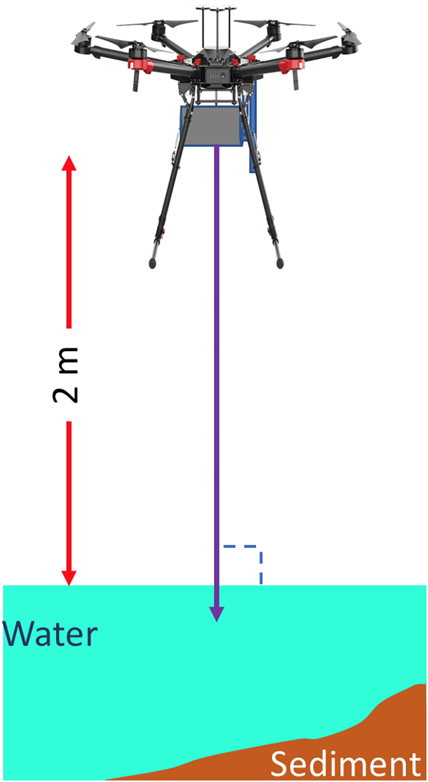

Introduction

The Raman scattering of the OH-stretching vibration of water has been used in several reports as an internal standard for fluorescence measurements in environmental sensing, and as a reference for signal strength or instrument performance.^1–11 This inelastic scattering from water has an intensity, polarization and spectral distribution that is well known, and its dependence on temperature, phase, salinity and other factors has been the subject of thorough studies.^12–14

Our group develops optical instrumentation and has recently worked on development of a remote chlorophyll sensor that mounts on a small uncrewed aircraft system (sUAS, also called an aerial drone). ^{5 15–18} This instrument will use a laser directed down into water from above and will measure 180^o water Raman backscatter as an internal standard for fluorescence signals. As a point of reference, our goal is to fly the sUAS at a mean altitude of 2 m above the surface of the water, with the laser at normal incidence to the mean water surface level as illustrated in Figure 1.

Figure 1.

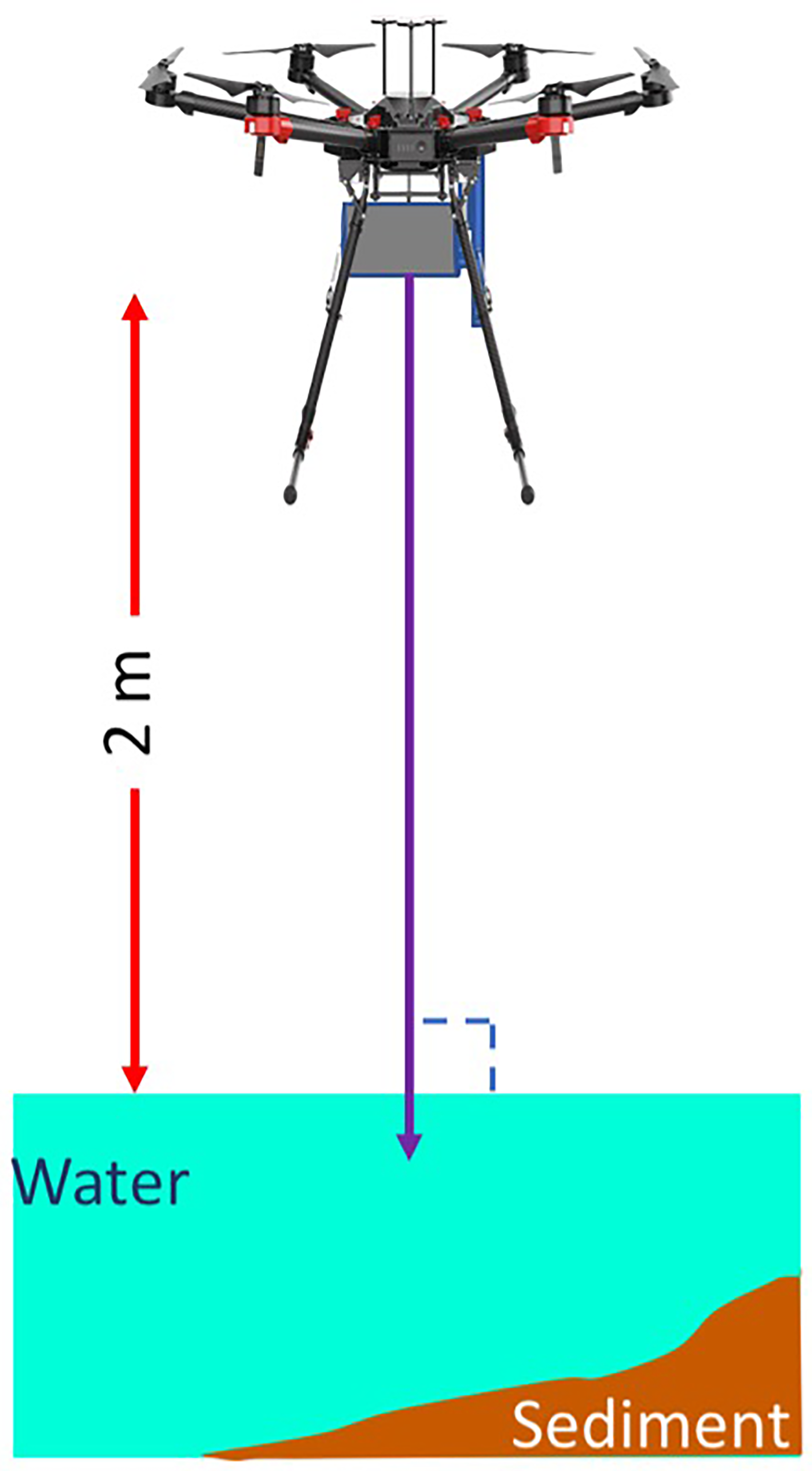
Schematic of the target optical configuration for aerial drone-deployed remote fluorescence sensor over a still water surface in shallow water.

Figure 2.

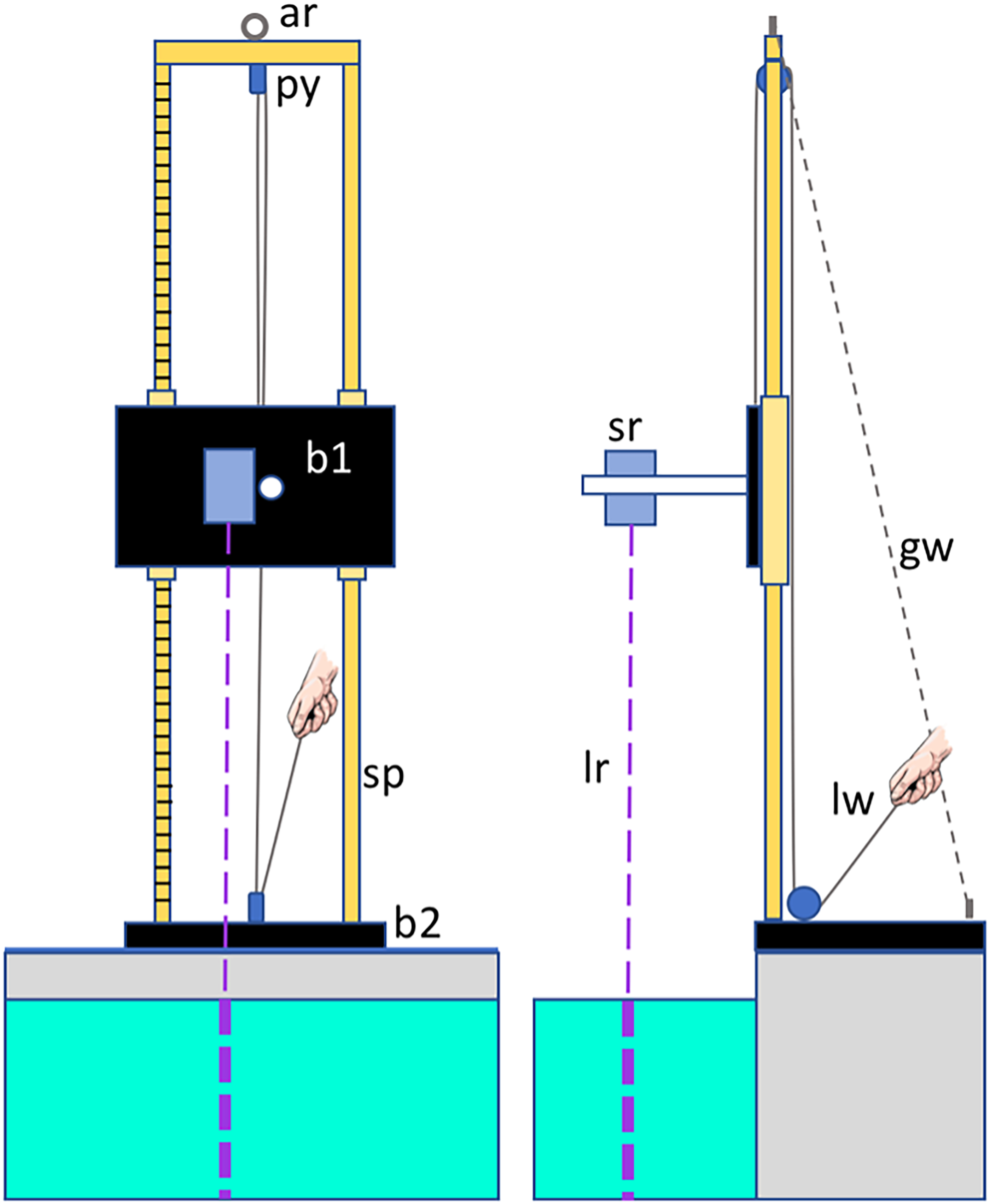
Apparatus for measuring height dependence of Raman signal strength. Components are PVC support poles (sp) and cross-brace at the top; guywires (gw) and their anchors (ar) for support; two pulleys (py) and a lift wire used to manually raise and lower the sensor (Ir); an optical breadboard (b1) with mount and two-axis tilt stage for the sensor. The laser (Ir) fires directly down into the water and the angle is adjusted until the laser retroreflects from the surface. One support post was graduated for ease of relative height measurement. The entire system is mounted on a larger optical breadboard (b2) and mounted at the edge of a tank, diving pool, or other body of water.

Pure water has low absorbance for much of the visible optical spectrum. In the natural environment, however, water is often colored or turbid or can be shallow so that sediment is observable. For these reasons, the depth of penetration of a laser source and the pathlength over which emission is collected may vary over a wide range. In addition, the measured signal is expected to be functionally related to the distance of the sensor from, and the angle of incidence the laser makes with, the water surface. These factors will vary with the altitude and attitude (orientation) of the sUAS above the water. Polarization of the source will also be relevant when the beam contacts the water surface at an oblique angle since reflection losses vary with the angle of incidence for s- and p-polarized light.

In this manuscript we report and model the water Raman signal strength as a function of vertical distance, water depth, and angle of incidence. The effect of height on measured Raman signal was observed using a short path length of water (∼12 cm) where the distance dependence might be expected to follow the inverse square law. This experiment was then repeated in a water body with a depth of 396 cm (13.0 ft.). At a reference height of 2 m, a Raman scattering signal in clear water was measured to be 22× larger for a depth of 396 cm than for a depth of 12 cm.

Two limiting cases for measurements in clear water can be identified corresponding to thin and thick sample conditions, with signal intensities proportional to the inverse square of distance and the inverse of distance, respectively. When neither limit is appropriate, the behavior of measurement systems is more difficult to calculate. An optical model is presented based on physical principles to account quantitatively for the variability in observed signals as a function of the water layer thickness and distance to the water surface. This model can be used to predict the performance of a remote sensor in clear, flat water conditions. This can be used to help select optical and electronic components for small remote optical systems, and provides expectations for the sensitivity, speed of data acquisition and signal to noise ratio of a planned instrument. The model can also be readily extended to account for sample absorption, angle of incidence and polarization effects.

Experimental

Materials and Methods

Figure 2 shows a schematic of a stationary apparatus with adjustable height that was constructed to hold and move the optical and electrical system components for the experiment. This structure consists of two 5.08 cm (2-in.) diameter and 3.48 m (10-ft.) long polyvinyl chloride (PVC) pipes secured to an optical board (b2). Matched holes for support pegs were drilled in increments on each pipe, beginning at 5.08 cm (2-in.) from the bottom of the pipes. From there, holes were drilled every 5.08 cm (2-in.) to a height of 96.52 cm (38-in.), after which holes were drilled every 10.16 cm (4-in.) to a height of 2.39 m (94-in.). Two additional PVC pipes 6.35 cm (2.5-in.) in diameter and 60.9 cm (2-ft.) long were slid over the 3.48 m (10-ft.) pipes and affixed to an optical breadboard (b1) on which the sensor was mounted. Optical bread board b1 can be moved vertically via a pulley system, with the shorter PVC pipes sliding over the 3.48 m (10-ft.) pipes. Pegs placed in the matched holes provide a fixed support for the shorter PVC pipes at specific heights, allowing for reproducible positioning of the sensor height. The only matched holes not used in this work were the two at a height of 60.96 cm (24-in.), where an internal support prevented the pegs from being placed securely into the holes.

Counterweights were added to the breadboard to balance the weight of the sensor and mounts on the pipes for easier movement, and a variety of optical components and tilt positioners were used to adjust the sensor and laser so the beam would be normal to the water surface as illustrated. A rotary mount with angle markings was used to adjust the angle of the sensor with respect to the normal for angle-dependent measurements once the surface normal orientation was established by back-reflection.

The optical system for the experiment consisted of an 80 mW continuous 450 nm diode laser (Laserlands, 16 mm blue laser dot module) modulated electronically at ∼7 Hz as the excitation source, an excitation filter (BrightLine Full Spectrum Blocking single-band bandpass filter, Semrock part no. FF01-451/106-25), a 450 nm reflecting beamsplitter (Semrock part no. FF510-Di02 25 × 36), and a bandpass filter centered on the water Raman band (BrightLine single-band bandpass filter, Semrock part no. FF02-531/22-25). The Raman measurement was recorded during alternating “on” cycles of the laser. Although only the water Raman channel was used, beamsplitters for two additional wavelengths were present in the instrument and not removed for this study. The laser itself is ∼95% polarized; this is not relevant for normal incidence measurements, but the relative s- and p-polarized intensities of the laser are provided below in the discussion of angle-dependent studies. A diagram of the instrument itself can be found in Supplemental Material for this report.

Accounting for losses in filters, more than 84% of the sample emission between 519 and 545 nm (overlapping the 450 nm excited water Raman band at approximately 517–543 nm) reaching the sensor is focused by an anti-reflective-coated f/1 aspheric lens (Edmund Optics 16-960) onto an avalanche photodiode (APD; Thorlabs APD440A), with rejection at the laser wavelength of an optical density of 12. The specifications for this detector indicate that it may become nonlinear at high optical powers (above 1 mW), but otherwise the linearity is not specified. A test of linearity was performed and data from the test are provided in Supplemental Material. Over the range of signal strengths studied here, the detector performance was indistinguishable from perfect linearity.

Short pathlength tests were performed in a laboratory setting using 12 cm-depth of deionized water. The water was contained in a glass beaker wrapped in black-anodized aluminum foil (Thorlabs) to reduce background light interference. Fluorescence of the glass was found to contribute to the signal, and this was eliminated by placing a square of black-anodized aluminum foil at the bottom of the water layer. The fluorescence of the aluminum foil was found to be minimal.

Long-pathlength tests were conducted at the 396 cm (13.0-ft.) depth of the diving pool at the Solomon Blatt Physical Education Center at the University of South Carolina in Columbia, SC. At the diving pool, the apparatus was assembled on the edge of the pool deck and was used to take repeat measurements at differing heights. The distance from the collection lens of the sensor to the water surface was estimated with a tape measure when the 5.08 cm (2-in.) matched peg holes were in use to provide an offset for all measurements. This estimated offset was ∼66 cm (26-in.). A sample of water from the pool was taken for a fluorescence analysis using a Horiba Fluoromax Plus spectrofluorometer (5 nm spectral bandpasses for excitation and emission) and found to be free of significant fluorescence with 450 nm excitation and possessing a clear and distinct water Raman band on a near-zero baseline.

The APD provides a range of amplification factors from 10–100, selectable with a dial on the side. In studies at the pool the Raman signal strength detected was slightly too high for the range set on the analog-to-digital converter, so the APD was not operated at its maximum gain. The gain was set so that the maximum signal would be on the order of 500 mV, and this gain setting was used for subsequent short pathlength tests as well. The exact gain setting was unknown as there are no indications on the detector.

Measurements were first taken moving the sensor from the lowest position to the highest, then from highest to lowest, with three complete repetitions. The sensor stayed at each height for thirty seconds while data was recorded. Dark-subtracted measurements were recorded at a rate of 3.5 Hz, controlled by an Arduino Nano BLE 33 Sense interfaced to a Raspberry Pi 3B+, and averaged over the period of measurement.

Results and Discussion

An example of raw data and the full set of average background-subtracted Raman signal measurements is provided in Supplemental Material for this work. Each value reported in figures here and in Table S1 in the Supplemental Material is based on the difference between the means of 16 384 measurements with the laser on and measurements with the laser off.

Figure 3 shows measured water Raman signal in mV as a function of the inverse square of distance to the water surface with a normal angle of incidence when the water is shallow (a depth of 12 cm). The system was focused at a distance of 200 cm for this measurement, and the collection lens–water surface distances tested ranged from 32 to 256 cm. The maximum signal detected (∼115 mV) corresponds to detecting approximately 164 pW of optical power in the OH Raman scatter band based a gain of 7.0 × 10⁸ V/W estimated from manufacturer specifications.

Figure 3.

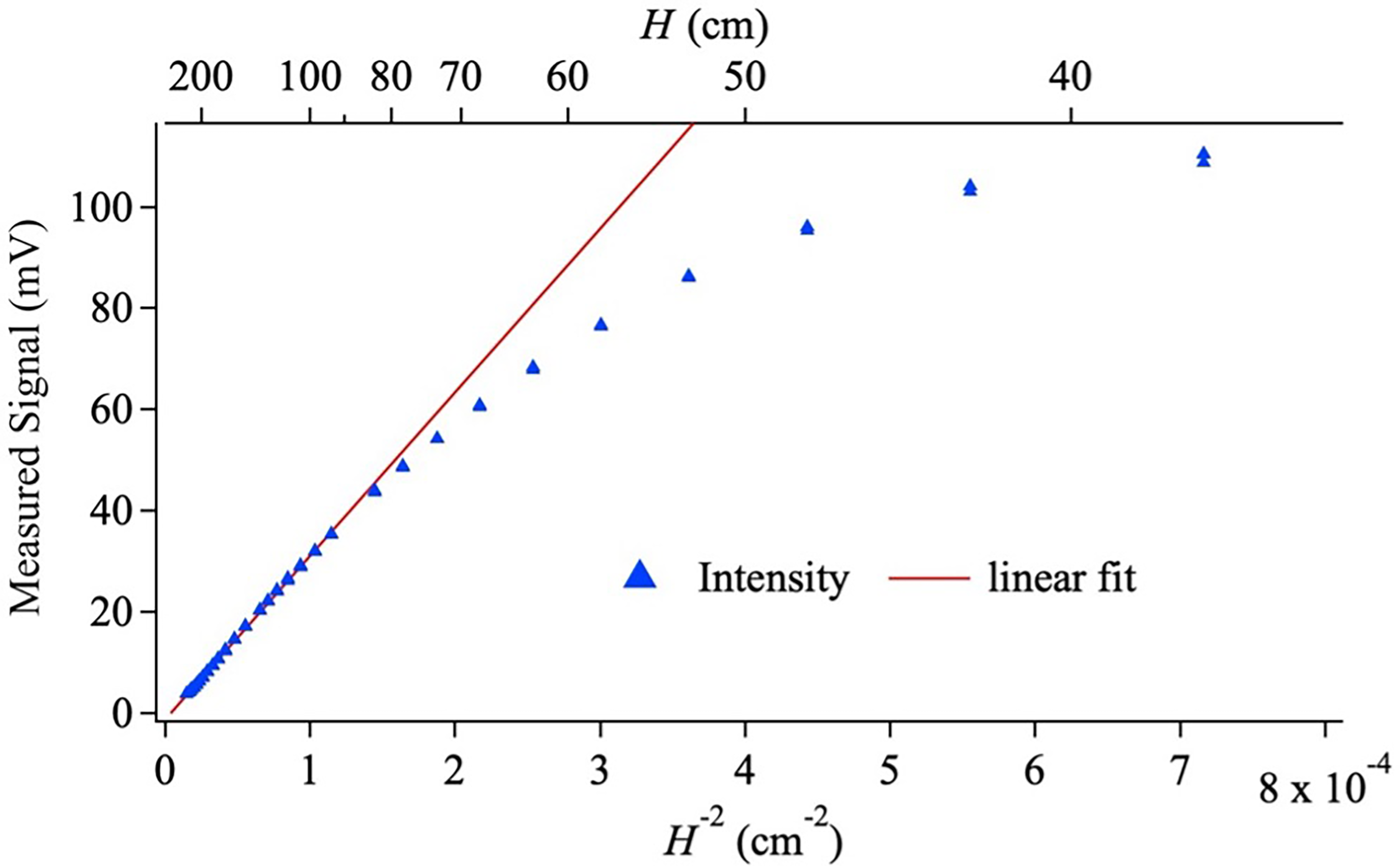
Measured shallow water OH Raman signal as a function of the inverse square of the distance to the water surface under the conditions: λ_ex = 450 nm at 75 mW; water layer thickness = 12 cm; detection lens aperture and focal length ∼2.5 cm/2 cm; detector diameter = 1 mm; detection wavelength band = 519–545 nm; detector conversion gain ∼7.0 × 10⁸ V/W in the detection band. The red line is the result of a fit between points with signal strengths of 3.79 mV and 35.29 mV. The top axis gives the corresponding value of H.

Figure 3 shows that for larger sample distances (245–80 cm) the signal strength measured for a shallow 12 cm-thick sample falls linearly with inverse distance as expected for a thin sample. For distances of 90 cm or less between the collection lens and the water surface (H^–2 = 1.2 × 10^–4 cm^–2) a significant deviation from this relationship is observed, and when the distance falls below 40 cm the signal strength clearly begins to plateau in the data. The linear region is interpreted to mean that the depth of focus is sufficient for all water Raman scattering to strike the active area of the detector, and that the distance is large enough for the 12 cm sample to behave as a “thin” sample. In the intermediate range the thickness of the sample becomes non-negligible, and the data begin to deviate from the inverse square rule. At even shorter distances, the depth of focus is not sufficient to capture all the scattered light on the 1 mm diameter detector, and a simple ray optics calculation shows that the disc of illumination begins to exceed the diameter of the detector when the distance between the collection lens (focused at a distance of 200 cm) and the water surface falls below ∼50 cm.

Figure 4 shows measured water Raman signal in deeper water (396 cm) as a function of sensor height (70–305 cm) above water plotted and fit in three different ways.

Figure 4.

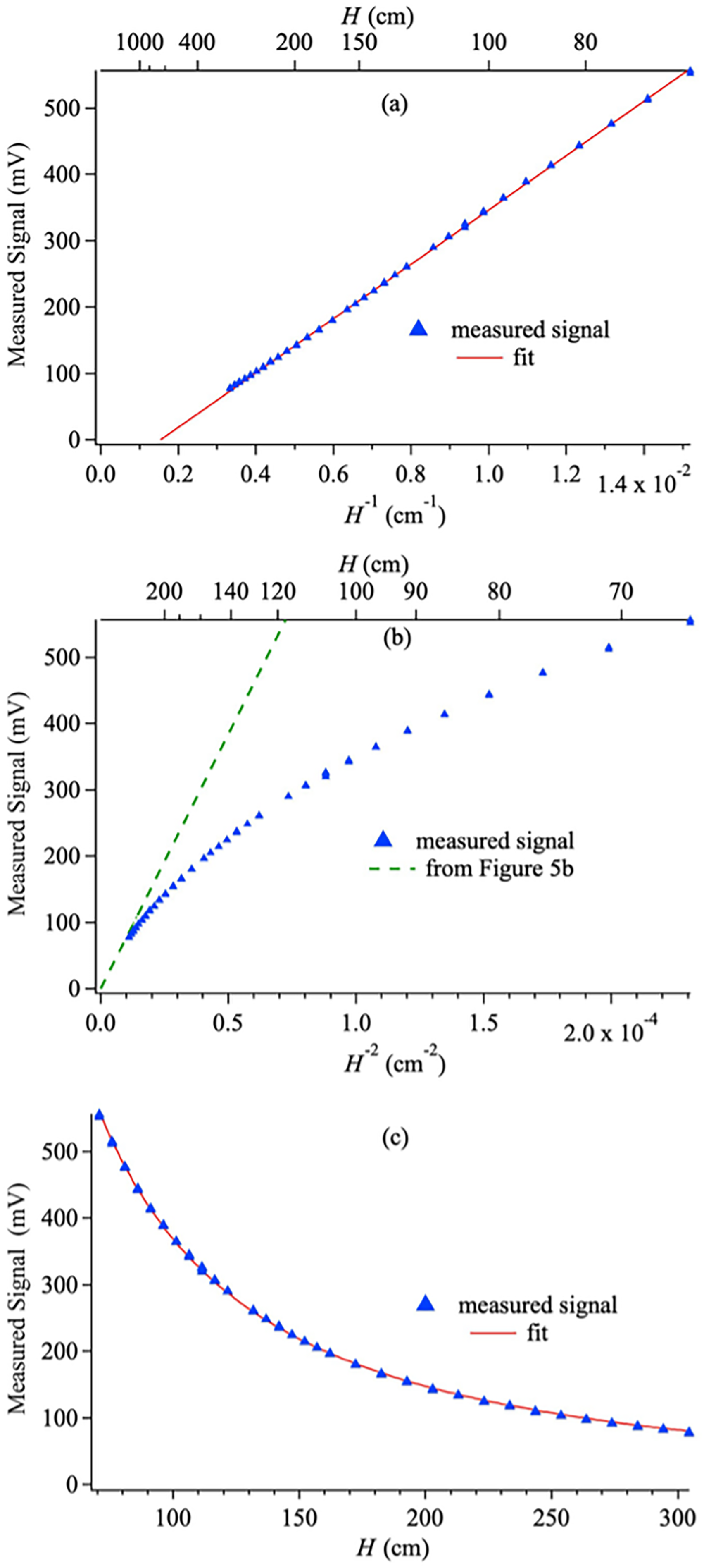
Deeper water OH Raman measured signals as a function of (a) the inverse of the distance to the water surface (with top axis of distance), (b) the inverse square of the distance (with top axis of distance), and (c) the distance. The red line in Figure 4a is fit between points with measured signals of 109 mV and 556 mV. Conditions are the same as in Figure 3 except the water layer thickness is 396 cm. The dashed green line in panel (b) represents the fit in Figure 5b. The red line in panel (c) uses the model developed in the text.

In Figure 4a, the data are fit to the inverse of the distance from the water surface to the sensor because this is the function that might be expected if the water layer were infinitely thick. The best-fit line fits the data well but does not pass through the origin and measurements begin to deviate from the line as H^–1 approaches zero. The 396 cm-thick sample is interpreted to appear experimentally thick at small values of H, but as H increases even a 4 m-thick water layer will eventually appear “thin” and begin to follow an inverse square relationship.

Figure 4b shows that at the maximum measured H of 305 cm for this study the point has not been reached where the data truly follows an inverse square law: the data is still curving toward the origin at the smallest measured value of H^–2. A dashed green line shows a fit to even larger distances based on Figure 5 (below) to give the reader an idea of what might be expected for the asymptotic behavior of the data points as they approach the origin.

Figure 5.

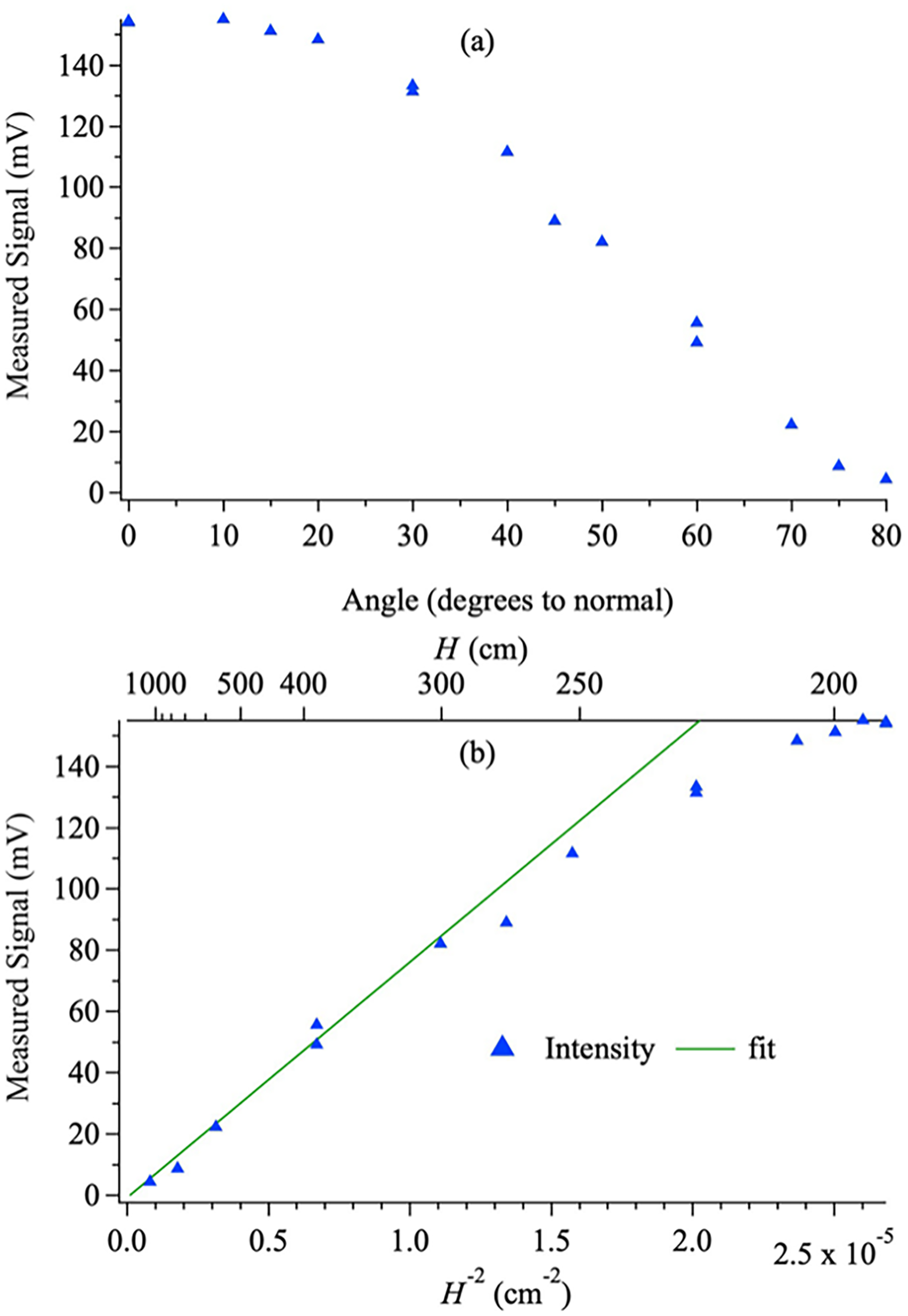
Measured water Raman signal from deep water as (a) a function of angle of incidence with a still water surface and (b) a function of the inverse squared distance to the water surface during the angle study (with a top axis giving the distance itself). The green line is the result of a fit between points with measured signals of 4.35 mV and 82.12 mV. The sensor was located 193 cm above the water surface with a laser that was ∼74% s-polarized. All other parameters are the same as in Figure 3. The fit in panel (b) appears in Figure 4b.

The final panel of Figure 4 shows a plot of measured signal versus H itself with a fit based on a new model (see Modeling section below). As shown in Figure 3, the minimum value of H in Figure 4b, 70 cm, is near the point at which the short path data deviates from an inverse square law, but before signal begins to plateau due to depth of field concerns as described above. Data could not be collected for this sample at distances less than 70 cm due to the distance between the pool deck and the water level at the diving pool.

Figure 5 shows the result of measurements taken at different angles of incidence with the water surface when the sensor was located at a height of 193 cm above the water surface at the diving pool. The depth of water was constant, but several factors complicate the interpretation of the angle data. First, the pathlength through the water changed across the measurement due to refraction at the water’s surface, a factor tending to increase the signal. Second, subsequent testing showed that the laser intensity was 25.9% p-polarized and 74.1% s-polarized relative to the plane of incidence in this angle-dependent study. The Raman scattering from the OH-stretching vibrations of water has a depolarization ratio near 0.156, ¹⁴ meaning that the scattering will be slightly less polarized than the laser itself. The polarization of the water Raman scattering in this experiment is calculated to be ∼32.4% p-polarized and ∼67.6% s-polarized.

The reflectance of water at normal incidence is ∼2.01%, which falls to 0 for p-polarized light at the air–water Brewster angle of 53.2° and then increases sharply beyond this angle. The air/water interface reflectance for s-polarized light increases monotonically with angle, reaching ∼46% at 80˚. Since most of the laser intensity was s-polarized, the reflection at the water surface, small and constant in Figures 3 and 4, will overall increase monotonically with increasing angle of the laser in this study, decreasing signal strength with angle, particularly for large angles. These pathlength and reflectance factors tend to partially cancel one another.

Figure 5a shows that even at a distance to the water surface calculated to be >1100 cm, the sensor was still detecting ∼4.4 mV of signal with 2.54 cm (1-in.) optics. The measured noise in the system was about 0.16 mV, giving a signal-to-noise ratio (SNR) of 27.5 with 3.5 Hz sampling of water Raman at this distance. Despite the numerous caveats of reflection, polarization and refraction, the data of Figure 5b fit an inverse square law well for distances greater than ∼400 cm, consistent with the normal incidence data of Figure 4b. The slope of the large-angle portion of Figure 5b appears in Figure 4b as a green line to show how closely they correlate with one another.

Modeling

Simple approximations are used to obtain an optical model for remote measurements in clear, still water as a function of distance from the water surface, depth of water, and angle of incidence. Figure 6 defines important model variables D, G, H, n, P, θ_i, and θ_P. In this figure, a lens with diameter D defines the acceptance angle for light. The exciting laser is assumed to be aligned on the lens axis with a diameter that is negligible compared to D and rays that are parallel. The distance between the sensor and the water surface, H, is further assumed to be large compared to D, reflection losses and attenuation of the laser and emission are negligible, all light collected by the lens is detected (a large-detector approximation), and emission from point P is isotropic. Dispersion of the refractive index of water is also neglected.

Figure 6.

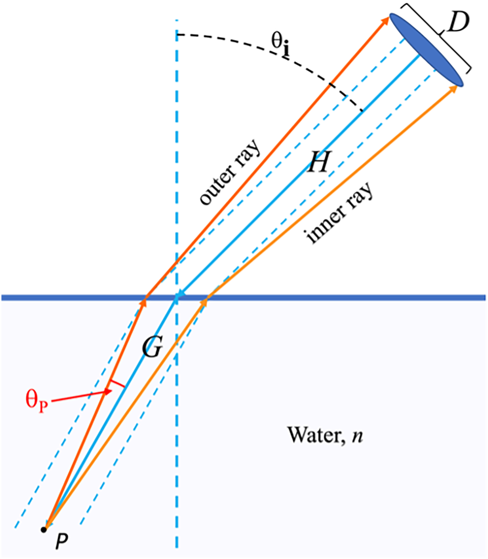
Schematic for the model of remote 180-degree backscattering emission from a layer or body of clear, flat water. A laser beam (solid blue line with arrows) emerging from the lens defines the points from which scattering or fluorescence can be generated. H is the distance the beam travels to the water surface, G is the distance it travels inside water to a point P where light emission occurs. θ _i is the angle of incidence between the laser and the normal to the water surface, defined relative to the surface normal, and n is the refractive index of water. θ _P is the half-angle of acceptance for light returning to the collection lens of diameter D in the place of incidence.

Some of the light emitted from point P due to light scattering or fluorescence travels a reverse path and enters the lens. The most extreme rays in the plane of the figure are labeled “inner” and “outer” and define the acceptance angle for light from point P.

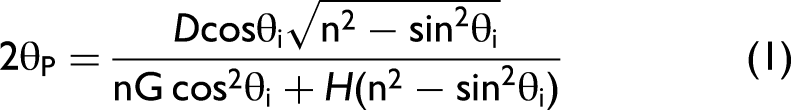
The Supplemental Material section for this report provides a detail of Figure 6 and derives the angle between the outer and central rays meeting at point P and the other variables defined in Figure 6 as:

$$2{\theta }_{\mathrm{P}}={\displaystyle \frac{D\cos {\theta }_{\mathrm{i}}\sqrt{{\mathrm{n}}^2-{\sin }^2{\theta }_{\mathrm{i}}}}{\mathrm{nG}{\cos }^2{\theta }_{\mathrm{i}}+H({\mathrm{n}}^2-{\sin }^2{\theta }_{\mathrm{i}})}}$$

(1)

It is easily shown that this is also the angle between the inner and central rays and is thus the half-angle of acceptance in the plane of incidence.

Modeling Long- and Short-Pathlength Data

To determine the solid angle over which light can be collected from point P, the half-angle of acceptance perpendicular to the plane of incidence in Figure 6 is required as well and is taken to be equal to Eq. 1 when θ_i = 0, or

$$2{\theta }_S={\displaystyle \frac{D}{\mathrm{G}+nH}}$$

(2)

where θ_S is defined to be the half-angle perpendicular to the plane of incidence. These two half-angles, θ_S and θ_P, define a coaxial elliptical cone extending from point P back toward the water surface. The solid angle subtended by such a cone is given exactly by Eq. 56 in Conway. ¹⁹ For remote measurement where H>>D, small angle approximations allow us to approximate the exact solution as a function of q_S and q_P:

$$\begin{array}{c}\mathrm{\Omega }({\theta }_{\mathrm{P}},{\theta }_{\mathrm{S}})\approx 2\pi -{\displaystyle \frac{4{\theta }_{\mathrm{P}}\mathrm{\Pi }({\alpha }^2,\mathrm{k})}{{\theta }_{\mathrm{S}}\sqrt{1+{\theta }_{\mathrm{S}}^2}}}\\ \alpha =\sqrt{1-{\displaystyle \frac{{\theta }_{\mathrm{P}}^2}{{\theta }_{\mathrm{S}}^2}}}\\ k=\sqrt{{\displaystyle \frac{{\theta }_{\mathrm{S}}^2-{\theta }_{\mathrm{P}}^2}{1+{\theta }_{\mathrm{S}}^2}}}\end{array}$$

(3)

where Π(α², k) is a complete elliptic integral of the third kind.

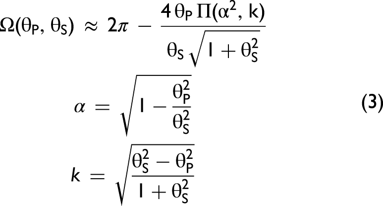
A second small angle approximation can be made as simply the solid angle subtended by an ellipse formed in a plane perpendicular to the axis of the coaxial elliptical cone:

$$\mathrm{\Omega }({\theta }_{\mathrm{P}},{\theta }_{\mathrm{S}})\approx \pi {\theta }_{\mathrm{P}}{\theta }_{\mathrm{S}}$$

(4)

The validity of these approximations can be established by comparison to the exact solution of Conway. ¹⁹ As an example, for small angles θ_S = 0.02 rad and θ_P = 0.01 rad, the exact formula gives a solid angle of 6.28308 × 10^–4 sr while Eq. 3 gives 6.28200 × 10^–4 sr and Eq. 4 gives 6.28319 × 10^–4 sr, errors of 0.017% and 0.0018%, respectively. The angles used in this example exceed those typical of a remote measurement with 2.54 cm (1-in.) optics, while the simplicity of Eq. 4 renders it particularly advantageous.

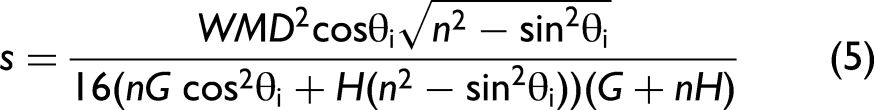
If the measured signal produced by light collected from point P is assumed to be proportional to the solid angle in Eq. 4, the proportionality constant must include factors for laser power, scattering efficiency and optical throughput. The dependence on laser power (W) should be linear, while the scattering efficiency should be given as the product of the power efficiency of water Raman scattering per unit length with the responsivity of the detection system integrated over the detected wavelength band, a factor called M below. Omitting other factors, e.g., interfacial reflections, absorbance of water, etc., the measured signal (s) from a single point excited by the laser is given approximately by:

$$s={\displaystyle \frac{WM{D}^2\cos {\theta }_{\mathrm{i}}\sqrt{n^2-{\sin }^2{\theta }_{\mathrm{i}}}}{16(nG\mathrm{co}{\mathrm{s}}^2{\theta }_{\mathrm{i}}+H(n^2-{\sin }^2{\theta }_{\mathrm{i}}))(G+nH)}}$$

(5)

The total measured signal (S) expected will be this quantity integrated from G = 0 through the total pathlength in water, G₀. The result of integrating Eq. 5 is provided in Supplemental Material, but this general result for all angles of incidence becomes undefined at normal incidence. Substituting θ _i  = 0 in Eq. 5 provides an equation that can be integrated for a particularly simple result at normal incidence:

$$S={\displaystyle \frac{WM{D}^2{G}_0}{16nH(G_0+nH)}}$$

(6)

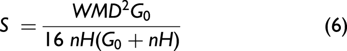
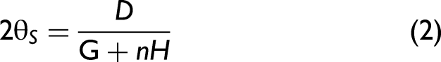
Equation 6 indicates that thin-sample conditions hold when G₀ << n H. Small G₀ also leads to low measured signals that are proportional to the inverse square of H. Thick sample conditions hold in the opposite limit, G₀ >> n H, yielding a signal that is independent of G₀ and inversely proportional to H.

Equation 6 is the model function used in Figure 4c above. For the fit in Figure 4c, 4 parameters were taken as constants: D = 2.54 cm, G₀ = 396 cm, n = 1.335, and W = 0.075 W. A single parameter providing scale, M, was fit to the data, giving M = (2.188 ± 0.003) × 10³ V W^–1 cm^–1. As mentioned above, even this parameter is not arbitrary: it represents the product of Raman scattering efficiency and detection system efficiency. Detection system efficiency for the APD itself is given in units of V/W; the efficiency of Raman scattering from water can be given in units of fractional conversion of the excitation into Raman scattering per cm of water pathlength, and these two factors provide the units of M.

M from the fit in Figure 4c can be compared to what is known about the optical system. The water Raman emission efficiency integrated over the entire OH Raman band for excitation at 450 nm has been previously ⁵ calculated to be 4.4 × 10^–6 cm^–1 based on literature values^15,20 and the estimated maximum conversion gain of the APD detector at 532 nm (the nominal detection wavelength) is 7.0 × 10⁸ V/W. Losses of 16% were estimated above from reflections in the optics, and another loss of 4% is expected from reflections at the water interface. The product of these values (Raman efficiency × APD gain × optical transmission) is 2.5 × 10³ V W^–1 cm^–1, an overestimation of the measured signal by 14%.

There is uncertainty in some of the parameters used in this calculation. For example, the actual aperture of the 1-in. lens is less than 2.54 cm due to the presence of retaining rings with a clear aperture of 2.28 cm, leading to an overestimation of the signal by ∼23%. Since the fluorescence of the water was measured and found to be minimal, the calculation above has been based entirely on Raman intensity, leading to underestimation of the measured signal from traces of fluorescence. The model also assumes the Raman scattering of water is isotropic when it is in fact weaker in the direction perpendicular to the plane defined by the polarization of the excitation and the direction of light propagation due to its small depolarization ratio. This underestimates the 180-degree Raman backscatter from water by ∼24%. Absorbance and particulate scattering have also been neglected in the model; including these two factors would affect the depth of penetration of light and reduce the observable Raman scattering, causing overestimation of signals if they are present. The gain setting of the APD for the deep-water experiments was reduced from its maximum value as described previously, also leading to overestimation of measured signal levels. Finally, there are also numerous points at which approximations have been made to get to Eq. 6. Given these uncertainties, some of which offset one another, the 14% overestimation of the measured signal is readily rationalized.

The short-path data of Figure 3 was repeated in a laboratory setting at the highest detector gain and is shown in Supplemental Material. A fit using the same model is given for H > 50 cm and it provides M = (2.29 ± 0.12) × 10³ V W^–1 cm^–1. The experimental conditions remove the uncertainty over the APD gain setting and the possible contribution of scattering and absorption but still overestimates the measured signal by about 8%.

Conclusion

Data has been presented for a remote water Raman sensor using 450 nm excitation and 2.54 cm (1-in.) optics at normal incidence in short and long pathlengths, and at a variety of angles. Fixed pathlengths follow an inverse square law for intensity when the remote distance to the sample is significantly larger than the sample pathlength and follow an approximate inverse distance model for short remote distances in thick samples. A model suited to calculating the remote Raman signal from clear, still water has been presented that fits data well for short and long pathlengths and a wide range of remote distances at normal incidence. The model also produces physical parameters that are consistent with the performance of components of the instrument and the measured intensity of Raman scattering from water.

Supplemental Material

sj-docx-1-asp-10.1177_00037028251394346 - Supplemental material for Pathlength, Altitude and Angle of Incidence Dependence of Remote Water Raman Scattering

Supplemental material, sj-docx-1-asp-10.1177_00037028251394346 for Pathlength, Altitude and Angle of Incidence Dependence of Remote Water Raman Scattering by Whitney E. Schuler, Paige K. Williams, Zechariah B. Kitzhaber, Caitlyn M. English, Tammi L. Richardson, Nikos Vitzilaios and Michael L. Myrick in Applied Spectroscopy