Sage Journals: Discover world-class research

Abstract

Baseline correction is a vital part of spectral preprocessing, especially for Raman spectra. Iterative polynomial fitting is an easy but less accurate way to find baselines compared to other methods such as wavelet transform and penalized least squares (PLS) methods. The polynomial fitting methods can also get distorted results in certain conditions. In this paper, a neural network model for detecting the trend of the baseline was proposed to improve the correction accuracy of the fitting methods. The model selects the function basis according to the baseline trend instead of using a fixed polynomial function to match the baseline for a more precise fit. We also propose a way to generate simulation data, these data can be used to train the neural network model. The model provides reliable results for real spectral data with noise. Our method provides a new idea to correct the baseline with a strange shape. In addition, we examine the limitations of conventional iterative polynomial fitting, adaptive iteratively reweighted PLS and explain why our approach surpasses these methods.

Graphical abstract

This is a visual representation of the abstract.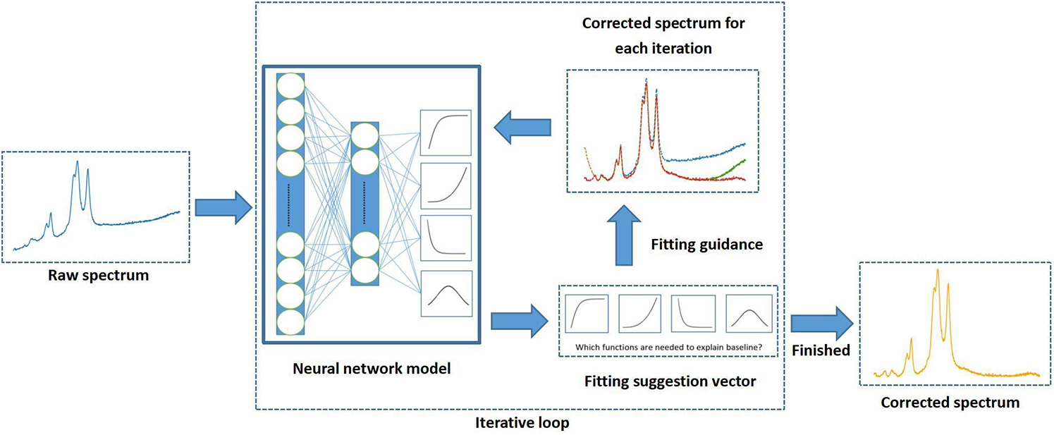

Keywords

Baseline correction neural network iterative fitting Raman spectra penalized least squares methods PLS methods

Introduction

Spectroscopy provides powerful support for chemical qualitative and quantitative analysis. Baselines due to complex factors, such as measurement error and impurity, make it hard to get detailed information from spectra. Therefore, baseline correction is a vital part of spectral preprocessing. To solve the problem, several methods have been proposed, including wavelet transform,^1,2 penalized least squares (PLS) methods such as asymmetrically reweighted PLS method,³ and adaptive iteratively reweighted PLS (airPLS).⁴ The precision of these techniques relies on the expertise of the researchers in configuring parameters, which can lead to subjective adjustments and reduced automation. Some methods based on fitting can also correct the baseline. These method principles are easy to understand, such as improved iterative polynomial method^5,6 and piecewise linear fitting.⁷ However, the correction accuracy will get worse if we choose an inappropriate fitting function.

Recently, baseline correction methods based on deep learning and neural networks have been proposed. The methods have various advantages, such as increased automation and decreased parameter debugging. Wahl et al.⁸ used a deep convolutional neural network to complete all pre-processing in a single step. Researchers also apply complex network structures to get the results more accurate; Baek et al.⁹ proposed ResUnet, a network structure that mixes ResNet and Unet to correct baseline.^10,11 Its correction performance evaluated by simulation data reached a high level. However, these applied methods have some potential problems. First, these models perhaps have low generalization. Although it is convenient to use the corrected spectrum as the output label of the model directly, it is difficult to judge whether these models learn how to identify the baseline or just memorize the training label. Second, the trained model uses a restricted number of feature nodes as model input and output.^8,9 Some spectral data nodes have to be discarded when their number is much more than that of the feature node to satisfy the input. Baek et al.⁹ compressed the length of the spectral data to 512 and sent them to the model. However, this compressing procedure causes irreversible damage to data and information loss. Most of the mineral Raman spectral data have thousands or more measuring points, but the output layer of these network models has only hundreds.^8,9,12 So, data compression is unavoidable for most of the spectral data when we use these deep learning methods. Last, the correction performance of these trained models on real data is not as good as that on simulation data. We analyze that the simulation baselines generated by the interpolation method cannot completely meet actual situations, and the outputs of these models are too specific to grasp the baseline characteristics.

We designed a method combining the neural network model and fitting. The neural network helps find a fitting function and improves the accuracy of the fitting strategy by setting parameter limits. Moreover, we proposed a modeling method for baseline to generate the simulation data and use it to train the neural network model. The trained model has a wider response to different baseline trends. The correction performance on real data is good and persuasive, even for those raw data with strong backgrounds and noise.

Mathematical Modeling of Baselines

Iterative fitting using the polynomial function of 5˚ will have an obvious shape transformation with the parameter changes, so baseline trends are more likely to be found during iterative polynomial fitting. However, not all the baselines can be fitted well by a polynomial function. A complex function with more parameters is more reliable for fitting.

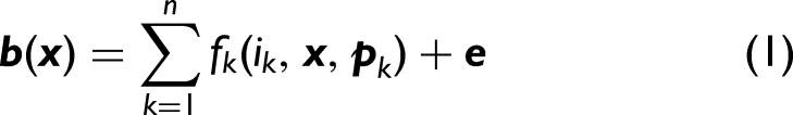
We define some mathematical functions as a basis to explain the baseline composition. Suppose we define n functions as the components of baseline, x represents the Raman shift vector, b represents the baseline expressed by x, f represents the mapping of the function basis, p represents the list of parameters for mathematical functions, e represents the error between the real baseline and the estimated one, i represents the intensity of each basis, and its value ranges from 0 to 1. The expression is shown in Eq. 1. This expression can express baselines with different trends by adjusting the intensity parameters i as well as the list of parameters p.

b (x) = \sum_{k = 1}^{n} f_{k} (i_{k}, x, p_{k}) + e

(1)

This expression explains the composition of the baseline better than a polynomial function even n is small. However, the computational efficiency will decrease, and the result may be stuck in a local value easily if we take all of the function parameters we choose to fit the baseline.

To solve the problem, we propose a classification neural network strategy to identify function participation. Classification strategies have been widely used in various tasks, such as spectral recognition^13,14 and image identification.¹¹ LeCun et al.¹⁵ took digits 0 to 9 as the output of the handwriting digital recognition network model, and Liu took hundreds of different minerals as the output of the spectral recognition network model.¹⁴ Here, we take the mathematical basis as output.¹⁶ Neural network modeling helps us remove some of the unnecessary functions to simplify the expression. A baseline may contain various basis functions, so it is considered a multi-label classification task.¹⁷

Model Training Strategy

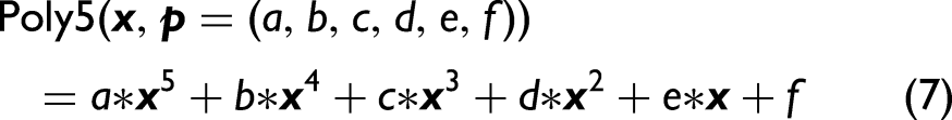
Simulation data are needed to train our neural network model because the real data is not enough. Some researchers choose the interpolation method to generate simulation baselines.⁹ In our experiment, we designed a new method according to Eq. 1 to generate simulation data. This data generation method is more appropriate for our neural network model. Gaussian peaks with random parameters are combined to form the pure spectrum. In the experiment, we choose three mathematical functions as a basis to build a network model to verify the method's feasibility. The three functions are expressed below:

Expo (i > 0, x, p = (ω > 0)) = i \cdot {(\frac{x}{max (x)})}^{ω}

(2)

N_expo (i > 0, x, p = (ω > 0)) = 1 - i \cdot {(\frac{x}{max (x)})}^{ω}

(3)

Gaussian (i > 0, x, p = (0 < μ < max (x), σ > 0) = i \cdot e^{(\frac{- {(x - μ)}^{2}}{2 σ^{2}})}

(4)

Equation 2 is the exponential function, Eq. 3 can be approximated as a negative exponential function, and Eq. 4 is the Gaussian function.¹⁸ The simulation baselines are composed of a combination of these functions. We adjust the parameter values in Eqs. 2–4 or discard certain functions to generate simulation baselines with different trends. To satisfy normalization, we divide the max value of every data to ensure the simulation value ranges from 0 to 1. It should be noted that more functions can improve the prediction accuracy of the model. In the online Supplemental material, we build a new model adding trigonometric functions to prove the extensibility of our method.

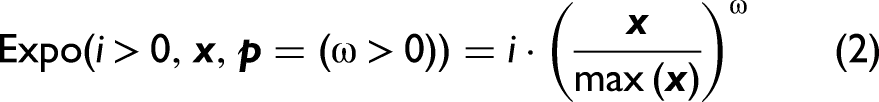
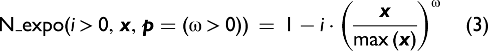
During the generation process, we make a statistic about the distribution of the parameter values and generate suitable parameter bounds for our fitting process later. We will give a label for each simulation data; it is a short vector to describe the function composition of the baselines. It has n elements representing the mathematical function types. Each simulation baseline is combined with some of the mathematical functions we defined. The label is set to all zero for pure spectrum. A parameter will change to one if the corresponding function is used to form the baseline. Figure 1 shows the data generation step. Each component changes its shape by adjusting parameters to form various baselines, but their tendency is similar because the basis functions are the same.

Figure 1.

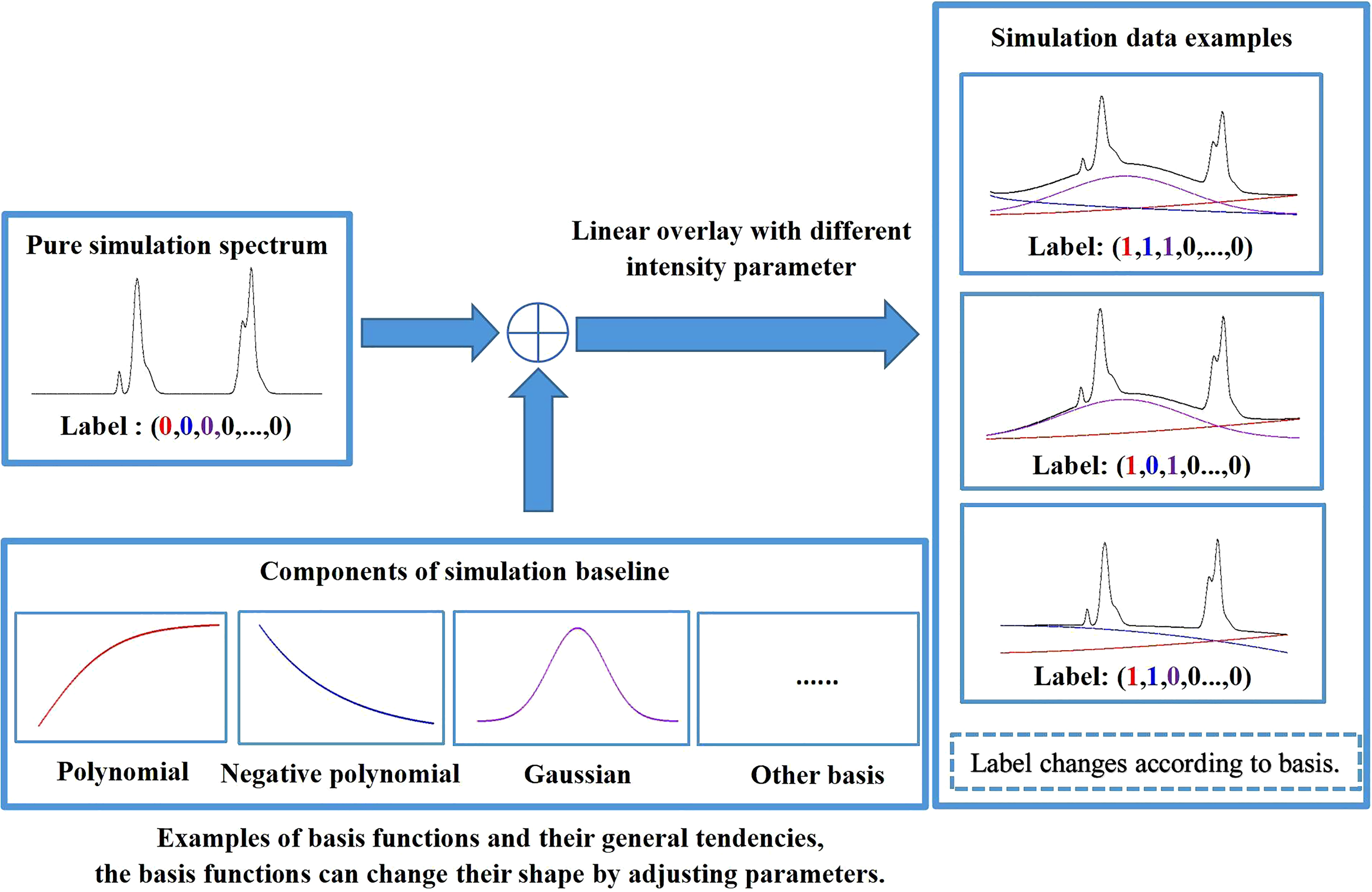
Procedure for generating simulation data.

We used these simulation data for model training. Our neural network was built and trained in Python using the Pytorch package. The main difference is that our model outputs a short vector expressing the participation of the basis function instead of a long one expressing a specific baseline. Next, we need to restore the short vector to a baseline, here we use the iterative fitting strategy.^4,5 The neural network model gives a group of appropriate functions to fit the baseline in each iteration. What we need to do is find a parameter list to minimize e in Eq. 1 using fitting. This task is completed by a built-in function in Python called “curve_fit,” which is mentioned in the online Supplemental material.

In general, the neural network is used to decide which basis functions are qualified for fitting the raw spectrum, the parameters of each basis function can be changed to adjust the specific fitting. Figure 2 shows the program in an iteration, the input layer is a raw spectrum, and the output is a vector representing the participation of the basis functions. For the same class of basis functions, their general tendency is similar, despite their specific parameters. This is why we take the general tendency of every basis function as the feature of the baseline.

Figure 2.

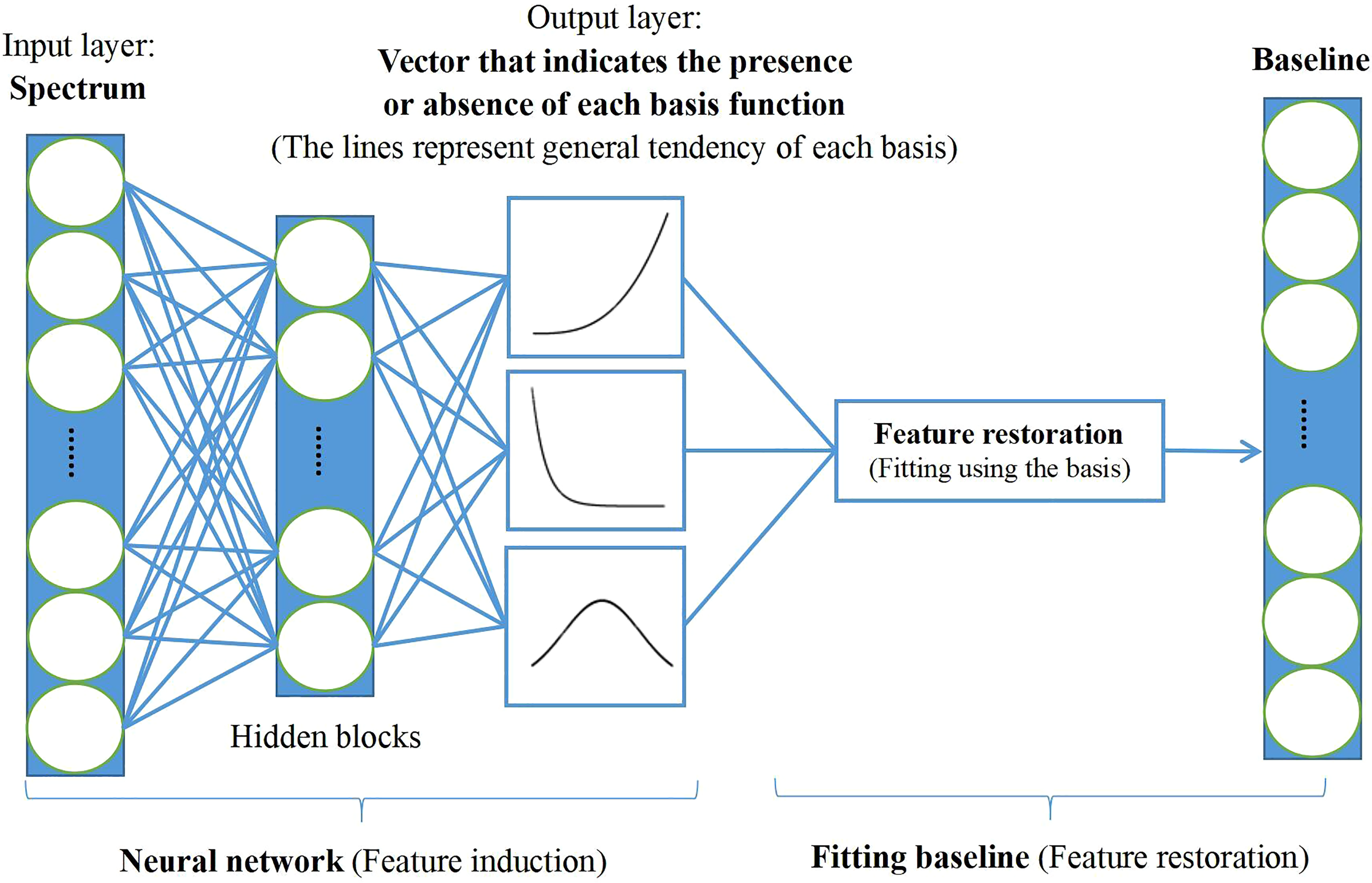
Structure of neural network model and the processing step in each iteration.

Performance of the Neural Network Model

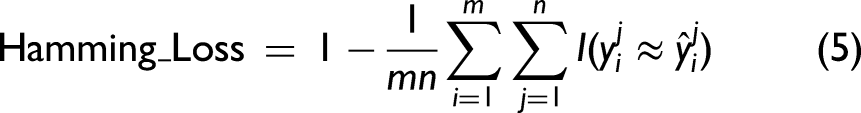
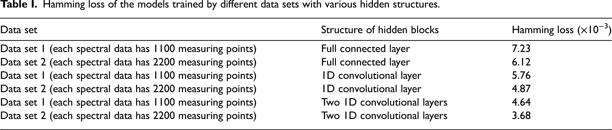
The performance of the neural network model reflects the reliability of the short vector the model gives us. We generated some new simulation data to test the accuracy of the output. In our experiment, we generated two data sets to train various neural networks with different structures. The main difference between the two data sets is the number of measuring points, the length of the data in two data sets are 1100 and 2200 separately. The performance of the model is evaluated by Hamming loss, which is an evaluation for multi-label classification. Assuming that a data set has m samples, each sample has n elements, $y_{i}^{j}$ represents the jth element of the ith sample, and ${\hat{y}}_{i}^{j}$ represents the jth element of the ith prediction vector. I is an indicator that returns 0 when $y_{i}^{j}$ approaching ${\hat{y}}_{i}^{j}$ , otherwise, it returns 1. In our experiment, we define that the element of the output vector approaches 1 when it is >0.5, otherwise, it approaches 0. Hamming loss is defined as the following equation:

Hamming_Loss = 1 - \frac{1}{m n} \sum_{i = 1}^{m} \sum_{j = 1}^{n} I (y_{i}^{j} \approx {\hat{y}}_{i}^{j})

(5)

We listed the hamming loss of three different network structures trained by two different data sets in Table I. The first model took a fully connected layer as a hidden layer, the second one took a one-dimensional (1D) convolutional layer as hidden blocks, and the last took two convolutional layers as hidden blocks. All hyperparameters were set to suitable values. The result shows that a specific spectral data set can improve the prediction accuracy of the model.

Table I.

Hamming loss of the models trained by different data sets with various hidden structures.

Data set	Structure of hidden blocks	Hamming loss (×10⁻³)
Data set 1 (each spectral data has 1100 measuring points)	Full connected layer	7.23
Data set 2 (each spectral data has 2200 measuring points)	Full connected layer	6.12
Data set 1 (each spectral data has 1100 measuring points)	1D convolutional layer	5.76
Data set 2 (each spectral data has 2200 measuring points)	1D convolutional layer	4.87
Data set 1 (each spectral data has 1100 measuring points)	Two 1D convolutional layers	4.64
Data set 2 (each spectral data has 2200 measuring points)	Two 1D convolutional layers	3.68

Correction Performance of the Whole Method

The correction performance for simulation data can be evaluated by mean absolute error (MAE), assuming that y and ŷ represent the true baseline and the baseline expressed by our method, l represents the number of measuring points of the data, the equation of MAE is shown in Eq. 6:

MAE = \sum_{i = 1}^{l} | y_{i} - {\hat{y}}_{i} | / l

(6)

In Eq. 6, we generated a new data set consisting of 100 simulation spectra as a test set to compare these methods, and 70% of the simulation baselines were generated in a way consistent with training data, and the rest of them were generated by interpolation.⁹ We compared our method with airPLS and iterative polynomial fitting. Here, we used a 5° polynomial function to fit the simulation data, the expression is shown in Eq. 7. All parameters in p are selected by fitting without limits.

Poly 5 (x, p = (a, b, c, d, e, f)) = a * x^{5} + b * x^{4} + c * x^{3} + d * x^{2} + e * x + f

(7)

In our experiment, the iterative polynomial method performed 10 iterations and we recorded the results with the smallest MAE during the process. For airPLS, we set the max number of iterations to 15 and the hyperparameter lambda (λ) 10, 100, 1000, 10 000 (log₁₀λ = 1, 2, 3, 4) separately, we record the result with the smallest MAE value. To make a statistic, we get an MAE from every test data from the data set, and we calculate the mean and standard deviation of the value of MAE. Table II shows these data measuring from airPLS,⁴ iterative polynomial method⁵ and our method. The following conclusions can be drawn from the table. First, our method has better correction performance than the other two methods because the mean value is smaller. Second, fitting methods are more reliable than airPLS, as they have a lower standard deviation.

Table II.

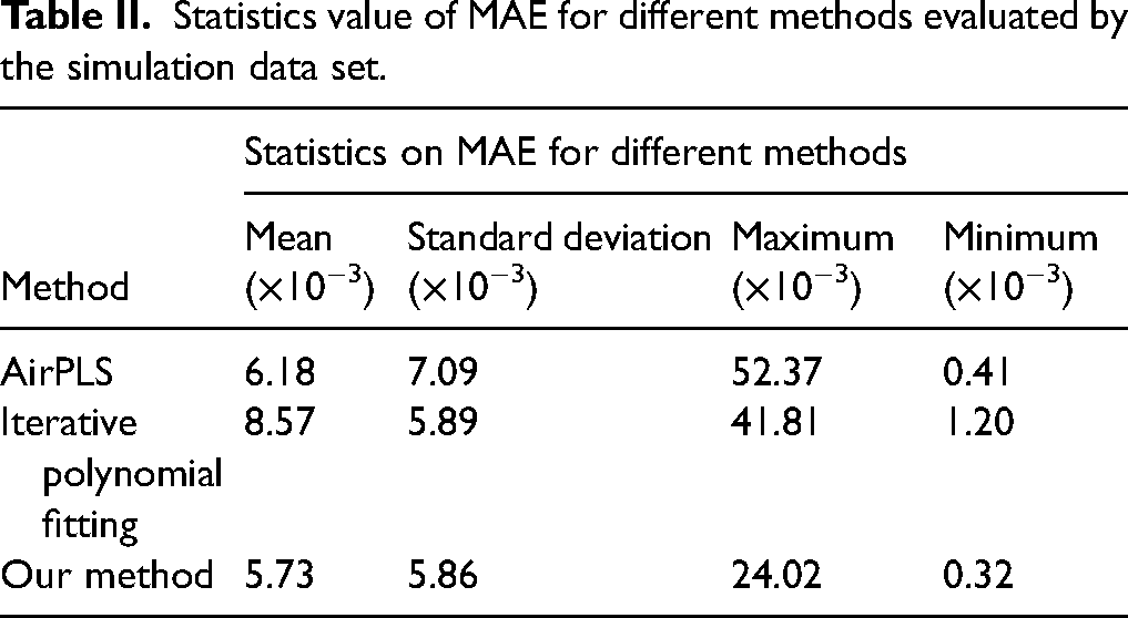
Statistics value of MAE for different methods evaluated by the simulation data set.

	Statistics on MAE for different methods
Method	Mean (×10⁻³)	Standard deviation (×10⁻³)	Maximum (×10⁻³)	Minimum (×10⁻³)
AirPLS	6.18	7.09	52.37	0.41
Iterative polynomial fitting	8.57	5.89	41.81	1.20
Our method	5.73	5.86	24.02	0.32

Why Our Method Has Better Correction Performance

In this part, we will show some examples in the test data set and discuss the reasons. These examples are shown in Figure 3. The baseline of Figure 3a is generated according to Eq. 1 while the baseline of Figure 3b is generated by interpolation. The results show that the simulation baselines can be corrected by all the methods. It indicates that our method can also correct the baseline generated by interpolation. In Figures 3c and 3d, there are some concave parts in the fitting results of iterative polynomial fitting, we speculate that these are the errors that accumulated during the iterations. In Figures 3e and 3f, the airPLS gets terrible results. Especially for Figure 3f, airPLS confuses the protruding part of the baseline with the characteristic peaks, we will give some explanations for these phenomena.

Figure 3.

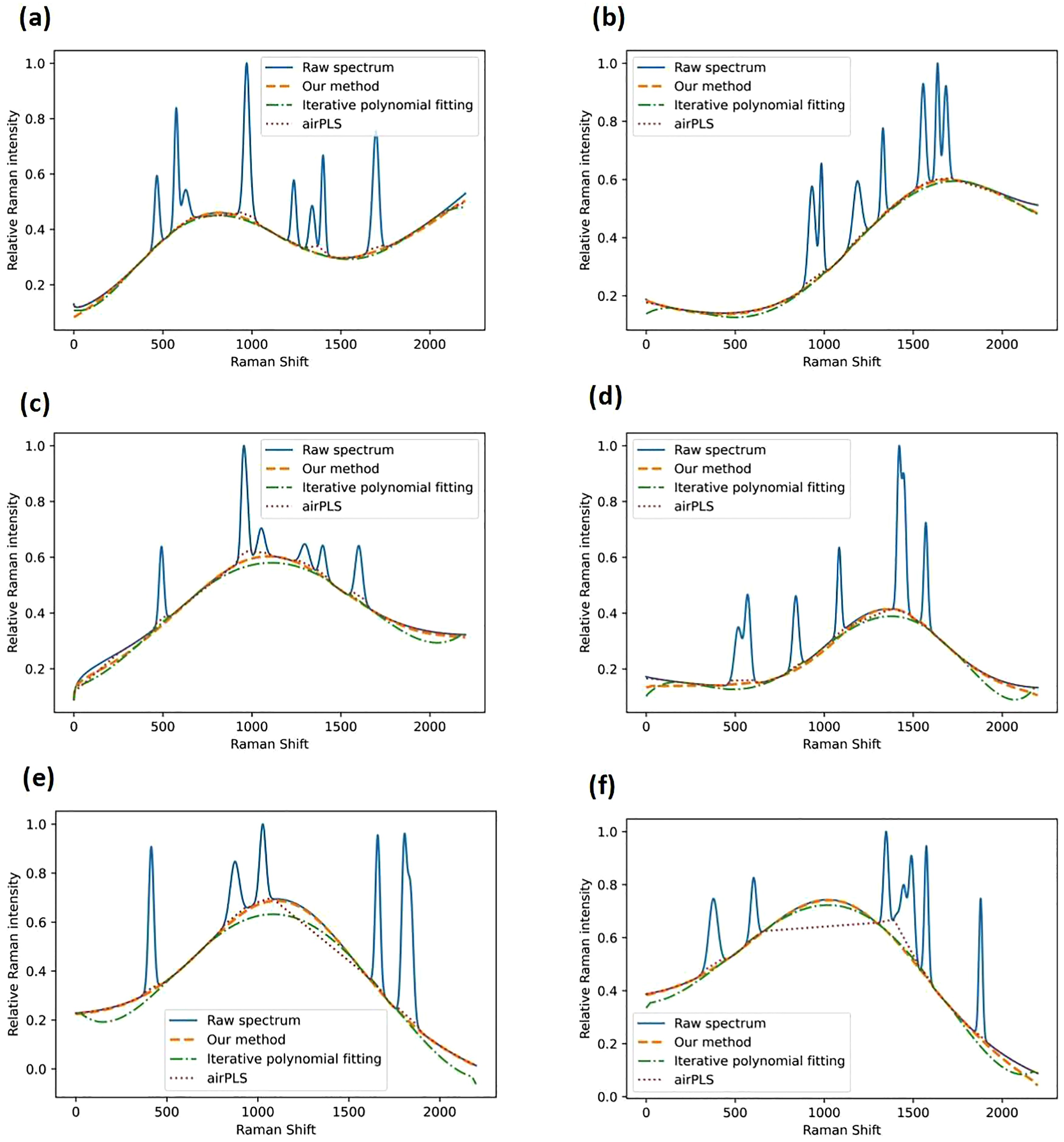
The corrected results of simulation data by iterative polynomial fitting, airPLS and our method. Panels (a) and (b) show the common baseline that can be corrected by all the methods, panels (c) and (d) show the distorted results from iterative polynomial fitting, and panels (e) and (f) show the distorted results from airPLS.

On the one hand, fitting is a good way to grasp the overall trend of the spectrum. However, it will get distorted results in conditions such as Figures 3c and 3d. Once it gets a wrong-fitting result in the first iteration, the error continues to accumulate in subsequent iterations. We show the iterative results of Figure 3d with different number of iterations in Figure 4a. It shows the results from iterative polynomial fitting. In order to fit the peak region well, the error in the edge part cannot be handled well in the first iteration, which is why the concave parts happen. With the iterative process, the fitting values that are greater than the actual baseline will converge to the baseline value. However, the fitting values that are smaller than the baseline in the first iteration will decrease continuously, causing distorted results. For our method, the neural network model changes the fitting function in each iteration to make sure the function has enough degrees of freedom and a suitable function to fit complex baselines well. In Figure 4b, our method adjusts the fitting trend to decrease the error caused by the iterative strategy.

Figure 4.

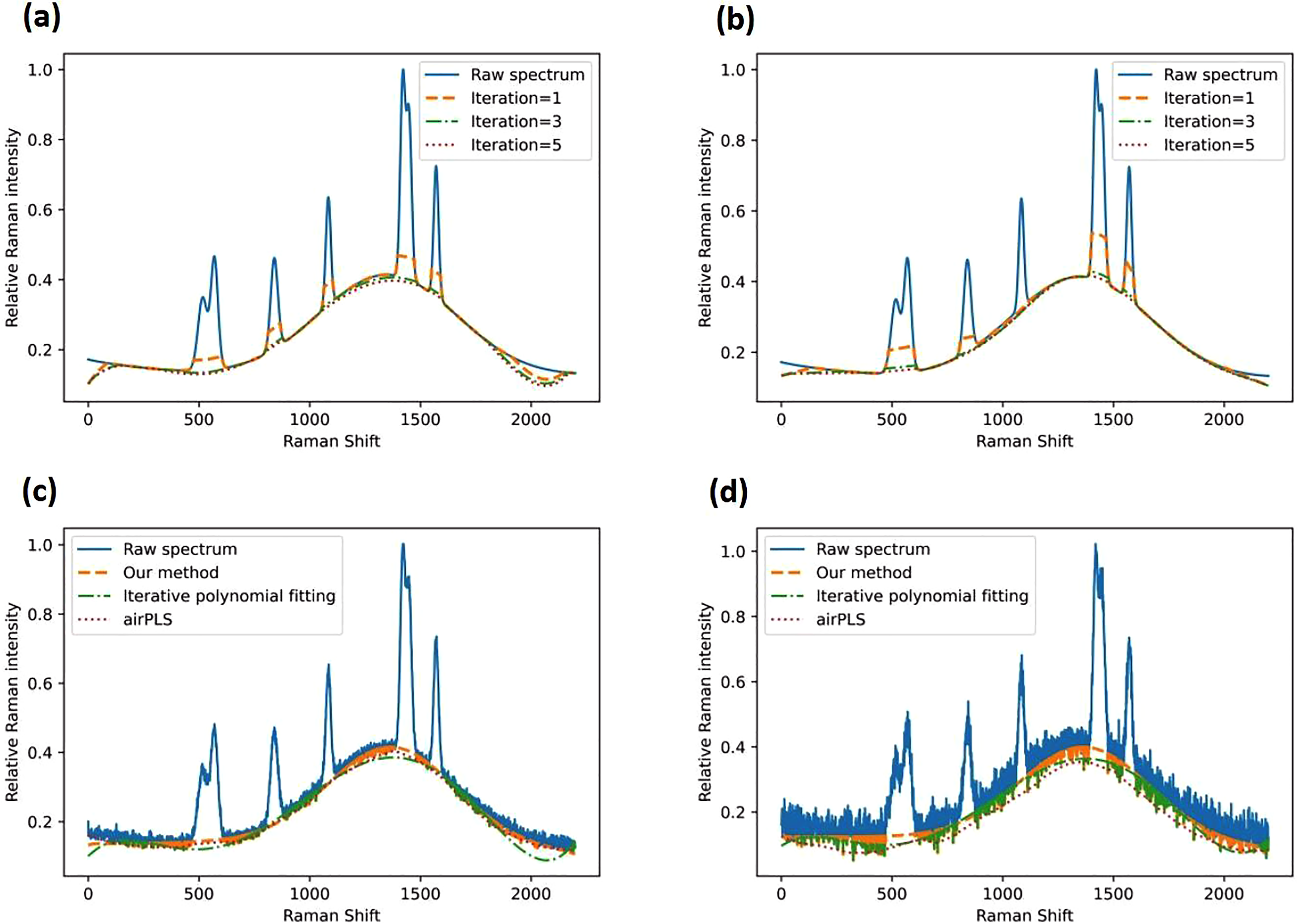
The fitted baselines with different iterations. (a) Iterative polynomial fitting. (b) Our method, with the corrected results with Gaussian noise. The simulation data with (c) weak noise. (d) Strong noise.

On the other hand, airPLS obtains baseline results through segmentation and local analysis but the overall trends will be easily neglected. This causes the method to get wrong answers when the baseline intensity is greater than that of characteristic peaks. In Figures 3e and 3f, airPLS cannot distinguish the characteristic peaks well from the bulge of the strong background. Although airPLS can adjust the lambda value to change the smoothness of the baseline, the problem cannot be solved. Moreover, Figures 4c and 4d show the spectrum in Figure 3d with different degrees of noise. We conclude that the effect of airPLS decreases as noise increases, while the fitting method is still applicable when there is noise in the spectrum.¹⁹

Correction Performance of the Real Data

We used some raw mineral Raman spectra in the RRUFF project to test the performance of our method. These raw data with baseline were measured by different organizations, we did not add any simulation baseline in these real examples. Figure 5 shows the corrected results of four different mineral Raman spectra: Mcguinnessite, Oxyphlogopite, Natrolite, and Chernovite-Y. The corrected results indicate that our method is relatively reliable. The concave parts around the edge have been improved a lot by our method compared with iterative polynomial fitting.

Figure 5.

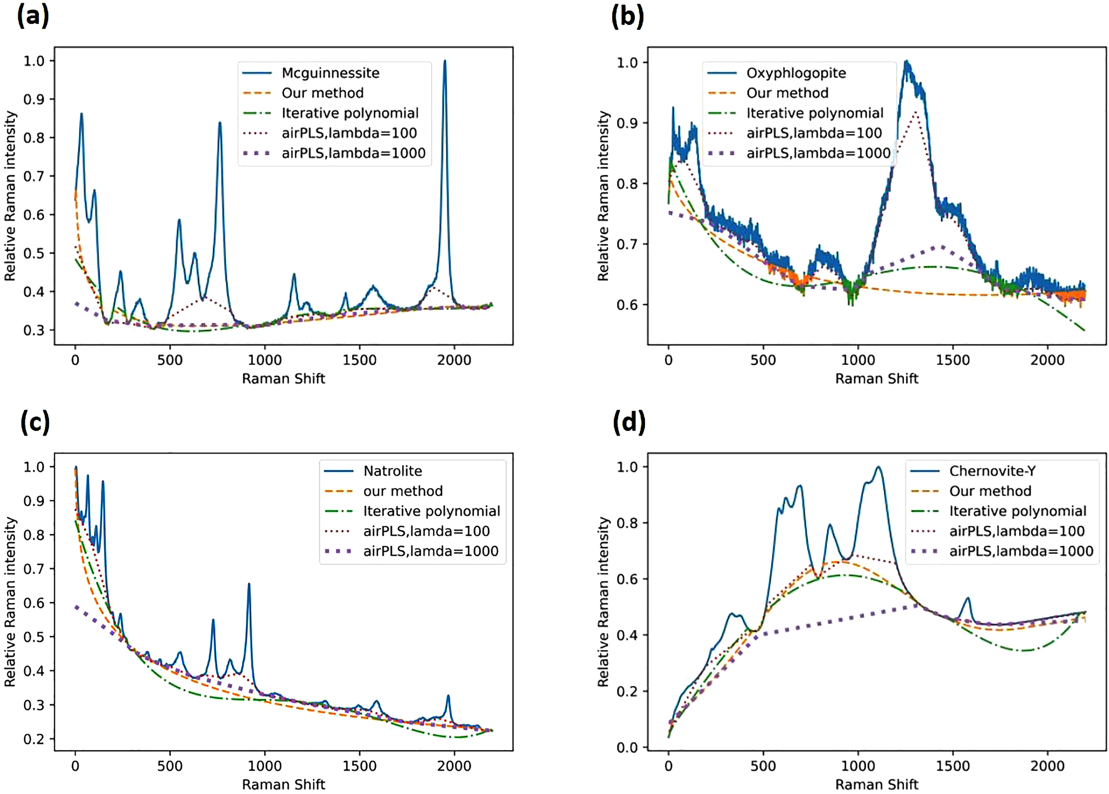
Corrected results of (a) Mcguinnessite, ID: R070082. (b) Oxyphlogopite, ID: R141079. (c) Natrolite, ID: R120124. (d) Chernovite-Y, ID: R070368. All raw data of the real samples in our article are provided by RRUFF.

Adaptive iteratively reweighted PLS (airPLS) gives different results depending on the lambda value. We plot baseline results when lambda is 100 and 1000, it is hard to tell which result is better. It seems that the results provided by airPLS are easily overcorrected in overlapping peak regions when lambda is small, while our method can preserve the peak area better. airPLS gets smoother results when lambda is large, it can improve the results such as Figure 5b. However, it is time-consuming to select the value of lambda, and the result may not improve when there is a strong background such as in Figure 5d, the method is also easily affected by noise. Our method gets the only result according to general tendency, so it is time-saving and has a strong noise immunity. We list more real examples in the online Supplemental material to show the performance of our method.

Use of the Neural Network Model in Our Method

Initially, we considered that an answer-oriented strategy was not good for a neural network model to improve its generalization, especially for the baseline correction task. We defined Eq. 1 to express the baseline and took the tendency of mathematical function as the output feature. The results showed that our method had a higher generalization, because the neural network is a tool for choosing a proper fitting function combined with our components. The training strategy guides the model on how to deduct the baseline trend, which is a process-oriented method. Later we consider it as an iterative fitting method to correct the baseline driven by the neural network model. Traditional iterative polynomial fitting uses a fixed polynomial function to fit the baseline during each iteration, while our method selects an appropriate function consisting of the basis functions during each iteration. It reduces the errors caused by inappropriate fitting function types. We need fewer artificial operations in the baseline correction task. The correction performance depends mainly on the neural network model, which can be improved in a relatively easy way. In conclusion, our method had both high generalization and automation.

How to Improve the Method

sThe neural network model decides the sensitivity and most of the accuracy of our method. It is vital for our model to identify the baseline trends. The model can be improved from the three aspects below. First, more baseline conditions should be considered as the data for training. For example, some baselines just have a slight intensity. This is easy to be ignored by our model if this condition is not in the training set. Second, we take the type of mathematical function as the model output. This training process teaches the neural network a way to identify the characteristics of the baseline. Therefore, more basis functions can also improve the model performance, such as trigonometric functions. We have added it as a part of our simulation baseline in the online Supplemental Material. Last, a complex structure such as ResNet or VGG-16 can improve sensitivity and generalization when there are too many mathematical function types. Our method will have higher generalization if we apply a more complex neural network structure. We believe that our method will have a better performance if we improve our neural network model in the ways above.

Conclusion

The paper proposes a baseline correction method combining neural networks and iterative fitting. Instead of using polynomials, we use different types of functions as basis functions, and the neural network chooses some of them to form a fitting function to reduce error. In this way, the model learns how to identify the feature of the baseline rather than memorize the corrected results directly. Using a neural network model, our iterative fitting method corrects the baseline by optimizing the fitting function. In contrast to iterative polynomial fitting, our method exhibits increased automation and generalization by selecting an appropriate function to fit the baseline in each iteration. In our method, data compressing can be avoided. Compared with those answer-oriented neural network models, it can preserve the data integrity in a more cost-effective way. Compared with other traditional methods, such as airPLS, redundant artificial operations can be avoided because the neural network model will guide most of the tasks. We have also proved that our method is insensitive to noise, it can get a clear baseline trend even for the data with high noise. In this paper, we just applied three different types of basis functions to train a simple model. We believe that our method will improve its performance if more basis functions participate in the model training.

Supplemental Material

sj-docx-1-asp-10.1177_00037028231212941 - Supplemental material for An Iterative Curve-Fitting Baseline Correction Method for Raman Spectra Driven by Neural Network

Supplemental material, sj-docx-1-asp-10.1177_00037028231212941 for An Iterative Curve-Fitting Baseline Correction Method for Raman Spectra Driven by Neural Network by Sicen Dong, Yuping Liu, Hanxiang Yu, Yuqing Wang and Junchi Wu in Applied Spectroscopy

Supplemental Material

sj-csv-2-asp-10.1177_00037028231212941 - Supplemental material for An Iterative Curve-Fitting Baseline Correction Method for Raman Spectra Driven by Neural Network

Supplemental material, sj-csv-2-asp-10.1177_00037028231212941 for An Iterative Curve-Fitting Baseline Correction Method for Raman Spectra Driven by Neural Network by Sicen Dong, Yuping Liu, Hanxiang Yu, Yuqing Wang and Junchi Wu in Applied Spectroscopy

Supplemental Material

sj-csv-3-asp-10.1177_00037028231212941 - Supplemental material for An Iterative Curve-Fitting Baseline Correction Method for Raman Spectra Driven by Neural Network

Supplemental material, sj-csv-3-asp-10.1177_00037028231212941 for An Iterative Curve-Fitting Baseline Correction Method for Raman Spectra Driven by Neural Network by Sicen Dong, Yuping Liu, Hanxiang Yu, Yuqing Wang and Junchi Wu in Applied Spectroscopy

Supplemental Material

sj-csv-4-asp-10.1177_00037028231212941 - Supplemental material for An Iterative Curve-Fitting Baseline Correction Method for Raman Spectra Driven by Neural Network

Supplemental material, sj-csv-4-asp-10.1177_00037028231212941 for An Iterative Curve-Fitting Baseline Correction Method for Raman Spectra Driven by Neural Network by Sicen Dong, Yuping Liu, Hanxiang Yu, Yuqing Wang and Junchi Wu in Applied Spectroscopy

Supplemental Material

sj-csv-5-asp-10.1177_00037028231212941 - Supplemental material for An Iterative Curve-Fitting Baseline Correction Method for Raman Spectra Driven by Neural Network

Supplemental material, sj-csv-5-asp-10.1177_00037028231212941 for An Iterative Curve-Fitting Baseline Correction Method for Raman Spectra Driven by Neural Network by Sicen Dong, Yuping Liu, Hanxiang Yu, Yuqing Wang and Junchi Wu in Applied Spectroscopy

Supplemental Material

sj-ipynb-6-asp-10.1177_00037028231212941 - Supplemental material for An Iterative Curve-Fitting Baseline Correction Method for Raman Spectra Driven by Neural Network

Supplemental material, sj-ipynb-6-asp-10.1177_00037028231212941 for An Iterative Curve-Fitting Baseline Correction Method for Raman Spectra Driven by Neural Network by Sicen Dong, Yuping Liu, Hanxiang Yu, Yuqing Wang and Junchi Wu in Applied Spectroscopy

Supplemental Material

sj-pkl-7-asp-10.1177_00037028231212941 - Supplemental material for An Iterative Curve-Fitting Baseline Correction Method for Raman Spectra Driven by Neural Network

Supplemental material, sj-pkl-7-asp-10.1177_00037028231212941 for An Iterative Curve-Fitting Baseline Correction Method for Raman Spectra Driven by Neural Network by Sicen Dong, Yuping Liu, Hanxiang Yu, Yuqing Wang and Junchi Wu in Applied Spectroscopy

Supplemental Material

sj-ipynb-8-asp-10.1177_00037028231212941 - Supplemental material for An Iterative Curve-Fitting Baseline Correction Method for Raman Spectra Driven by Neural Network

Supplemental material, sj-ipynb-8-asp-10.1177_00037028231212941 for An Iterative Curve-Fitting Baseline Correction Method for Raman Spectra Driven by Neural Network by Sicen Dong, Yuping Liu, Hanxiang Yu, Yuqing Wang and Junchi Wu in Applied Spectroscopy

Supplemental Material

sj-csv-9-asp-10.1177_00037028231212941 - Supplemental material for An Iterative Curve-Fitting Baseline Correction Method for Raman Spectra Driven by Neural Network

Supplemental material, sj-csv-9-asp-10.1177_00037028231212941 for An Iterative Curve-Fitting Baseline Correction Method for Raman Spectra Driven by Neural Network by Sicen Dong, Yuping Liu, Hanxiang Yu, Yuqing Wang and Junchi Wu in Applied Spectroscopy

Footnotes

Declaration of Conflicting Interests

The authors declared no potential conflicts of interest with respect to the research, authorship, and/or publication of this article.

Funding

The authors disclosed receipt of the following financial support for the research, authorship, and/or publication of this article: This study was supported by National Natural Science Foundation of China (Grant No. 61905047), and Fundamental Research Funds for the Central Universities of China (Grant No. 3072021CF2510).*

ORCID iD

Sicen Dong

Supplemental Material

All supplemental material mentioned in the text is available in the online version of the journal.

References

Jiang

Shen

, et al. “A Background Elimination Method Based on Wavelet Transform for Raman Spectra”. Chemom. Intell. Lab. Syst. 2007. 85: 94–101. 10.1016/J.Chemolab.2006.05.004

Qian

Hao

. “A Fully Automated Algorithm of Baseline Correction Based on Wavelet Feature Points and Segment Interpolation”. Opt. Laser Technol. 2017. 96: 202–207. 10.1016/J.Optlastec.2017.05.021

Baek

S.-J.

Park

Ahn

Choo

. “Baseline Correction Using Asymmetrically Reweighted Penalized Least Squares Smoothing”. Analyst. 2015. 140: 250–257. 10.1039/C4AN01061B

Zhang

Chen

Liang

. “Baseline Correction Using Adaptive Iteratively Reweighted Penalized Least Squares”. Analyst. 2010. 135: 1138–1146. 10.1039/B922045C

Feng

Zhu

Shen

Cong

. “The Method of Baseline Drift Correction of Raman Spectrum Based on Polynomial Fitting”. Comput. Appl. Chem. 2009. 26(06): 759–762. 10.16866/J.Com.App.Chem2009.06.017

Jiang

Wang

Hao

. “An Improved Iterative Polynomial Fitting Algorithm for Baseline Correction in X-ray Spectrum”. Adv. Sci. Technol. 2021. 105: 90–98. 10.4028/www.scientific.net/ast.105.90

Zhao

Guo

, et al. “Baseline Correction of UV Raman Spectrum Based on Improved Piecewise Linear Fitting”. Spectrosc. Spectral Anal. [Guangpuxue Yu Guangpu Fenxi]. 2020. 40(06): 1862–1869. 10.3964/J.Issn.1000-0593(2020)06-1862-07

Wahl

Sjödahl

Ramser

. “Single-Step Preprocessing of Raman Spectra Using Convolutional Neural Networks”. Appl. Spectrosc. 2020. 74(4): 427–438. 10.1177/0003702819888949

Chen

Son

Park

Baek

. “Baseline Correction Using a Deep-Learning Model Combining Resnet and Unet”. Analyst. 2022. 147: 4285–4293. 10.1039/D2AN00868H

10.

Zhang

Ren

Sun

R.J.

. “Deep Residual Learning for Image Recognition”. Proceedings of: The IEEE Conference on Computer Vision and Pattern Recognition. Las Vegas, Nevada; 27–30 June 2016. Pp. 770–778. 10.1109/CVPR.2016.90

11.

Ronneberger

Fischer

Brox

. “U-Net: Convolutional Networks for Biomedical Image Segmentation”. Paper presented at: International Conference on Medical Image Computing and Computer Assisted Intervention (MICCAI). Munich, Germany; 5–9 October 2015. Pp. 234–241. 10.1007/978-3-319-24574-4_28

12.

Liu

. “Adversarial Nets for Baseline Correction in Spectra Processing”. Chemom. Intell. Lab. Syst. 2021. 213: 104317. 10.1016/j.chemolab.2021.104317

13.

Luo

Juergen

Thomas

. “Deep Learning for Raman Spectroscopy: A Review”. Analytica. 2022. 3: 287–301. 10.3390/analytica3030020

14.

Liu

Margarita

Lorna

Michael

, et al. “Deep Convolutional Neural Networks for Raman Spectrum Recognition: A Unified Solution”. Analyst. 2017. 142(21): 4067–4074. 10.1039/C7AN01371J

15.

LeCun

Boser

Denker

J.S.

Henderson

, et al. “Backpropagation Applied to Handwritten Zip Code Recognition”. Neural Computation. 1989. 1(4): 541–545. 10.1162/neco.1989.1.4.541

16.

Ivan

Dmitr

Timofey

Timur

, et al. “An Approach for Feature Selection with Data Modelling in LC-MS Metabolomics”. Anal. Methods. 2020. 12(28): 3582–3591. 10.1039/D0AY00204F

17.

Prapowo

S.A.

Kang

Mubarok

M.S.

“An Implementation of Support Vector Machine on the Multi-Label Classification of English-Translated Quranic Verses”. J. Comput. Sci. 2019. 15(12): 1752–1758. 10.3844/Jcssp.2019.1752.1758.

18.

H.G.

Park

D.J.

Chang

D.E.

Hyunwoo

. “An Effective Baseline Correction Algorithm Using Broad Gaussian Vectors for Chemical Agent Detection with Known Raman Signature Spectra”. Sensors. 2021. 21(24): 8260. 10.3390/s21248260

19.

Bai

Xia

Zhang

W.D.

, et al. “Improved Baseline Correction Method Based on Polynomial Fitting for Raman Spectroscopy”. Photonic Sen. 2018. 8(4): 332–340. 10.1007/S13320-018-0512-Y

Supplementary Material

Please find the following supplemental material available below.

For Open Access articles published under a Creative Commons License, all supplemental material carries the same license as the article it is associated with.

For non-Open Access articles published, all supplemental material carries a non-exclusive license, and permission requests for re-use of supplemental material or any part of supplemental material shall be sent directly to the copyright owner as specified in the copyright notice associated with the article.

0.00 MB

0.02 MB

6.85 MB

7.35 MB

0.02 MB

0.76 MB

0.32 MB

0.17 MB

6.71 MB