Sage Journals: Discover world-class research

Abstract

Soil analysis to estimate soil fertility parameters is of great importance for precision agriculture but nowadays it still relies mainly on complex and time-consuming laboratory methods. Optical measurement techniques can provide a suitable alternative. Raman spectroscopy is of particular interest due to its ability to provide a molecular fingerprint of individual soil components. To overcome the major issue of strong fluorescence interference inherent to soil, we applied shifted excitation Raman difference spectroscopy (SERDS) using an in-house-developed dual-wavelength diode laser emitting at 785.2 and 784.6 nm. To account for the intrinsic heterogeneity of soil components at the millimeter scale, a raster scan with 100 individual measurement positions has been applied. Characteristic Raman signals of inorganic (quartz, feldspar, anatase, and calcite) and organic (amorphous carbon) constituents within the soil could be recovered from intense background interference. For the first time, the molecule-specific information derived by SERDS combined with partial least squares regression was demonstrated for the prediction of the soil organic matter content (coefficient of determination R² = 0.82 and root mean square error of cross validation RMSECV = 0.41%) as important soil fertility parameter within a set of 33 soil specimens collected from an agricultural field in northeast Germany.

Graphical Abstract

Keywords

Shifted excitation Raman difference spectroscopy SERDS fluorescence removal dual-wavelength diode laser soil constituents soil organic matter

Introduction

In modern agricultural practice, the concept of precision agriculture^1,2 is becoming increasingly important on a global level, for example, in terms of securing the food supply for a steadily increasing world population. Controlled site-specific and demand-oriented application of fertilizer and pesticides can ensure the sustainable use of limited resources and is, at the same time, crucial for environmental protection.³ For the successful implementation of precision agriculture, detailed knowledge of soil fertility parameters, for example, nutrient and organic matter contents, is essential to determine fertilizer demands. However, current standard procedures for soil testing in many countries mainly rely on the collection of one mixed sample from large areas in the order of 3 ha or more^4,5 followed by subsequent standard laboratory analysis. Due to the natural and anthropogenic soil variability at field scale⁶ and even down to the range of meters,⁷ a larger number of samples would ideally be required to enable farmers to make data-driven and demand-oriented management decisions about crop choice, planting time, fertilizer application rates, or irrigation.⁸ Unfortunately, a simple increase of the sample quantity is not practically feasible due to the time-consuming and expensive nature of conventional laboratory analysis.⁹

To address these unmet needs of precision agriculture for soil data at high spatial resolution, the application of advanced proximal sensing methods is required. With this goal in mind, the multidisciplinary project consortium, “Intelligence for Soil (I4S)–Integrated System for Site-Specific Soil Fertility Management”, funded within the German national program “BonaRes: Soil as a Sustainable Resource for the Bioeconomy”, is seeking to develop an integrated sensor system for in situ field application by combining a range of complementary measurement techniques with individual benefits. Selected atomic spectroscopic methods include X-ray fluorescence,¹⁰ laser-induced breakdown spectroscopy,^11–13 or gamma spectroscopy,^14,15 whereas molecular spectroscopic techniques comprise mid-infrared,⁴ near-infrared,¹⁶ and Raman spectroscopy.¹⁷

While atomic spectroscopy can reveal the total mass fractions of elements, their binding form within the soil cannot be determined by such methods.¹¹ Thus, complementary techniques to derive molecule-specific information of individual soil constituents are required, ideally with the intention to combine both approaches.¹⁰ Infrared spectroscopy can provide such molecular data but generally suffers from interference by water. This is not problematic when analyzing dried samples in the laboratory but could become a potential issue for in situ investigations directly on agricultural fields where a wide variety of moisture conditions can be present.¹⁸ Raman spectroscopy can provide a molecular fingerprint of the sample but shows only weak interference from water in the fingerprint spectral range. Conventional Raman spectroscopy is, however, rarely applied in the area of soil analysis as the intense fluorescence interference inherent to soil can easily superimpose the Raman spectroscopic signature making investigations challenging^19,20 or even impossible.²¹ One way to address the fluorescence issue is the application of excitation wavelengths in the deep ultraviolet spectral range below 250 nm. A serious drawback of this excitation with high-energetic laser photons is the radiation-induced damage of specimens that has been reported, particularly for organic compounds.²²

Shifted excitation Raman difference spectroscopy (SERDS)^23,24 is a powerful physical approach to separate the characteristic molecular fingerprint from interfering contributions. The basic principle behind SERDS is that the sample is consecutively excited at two slightly different excitation wavelengths. The characteristic Raman signals will follow the shift in excitation wavelength while static interfering contributions remain virtually unchanged. A following subtraction of the two recorded Raman spectra thus provides a neat way of separating the Raman spectroscopic fingerprint from background interferences. The technique does not only address the above-mentioned fluorescence issue²⁵ but also the interference from ambient light,²⁶ a topic of particular relevance for investigations outside laboratory environments.²⁷ We have recently demonstrated in a proof-of-concept study that SERDS can be successfully applied for the qualitative investigation of soil enabling the identification of different mineral constituents.¹⁷

In this paper, for the first time SERDS, using a dual-wavelength diode laser emitting at 785.2 and 784.6 nm combined with a raster scan approach comprising 100 individual measurement spots per sample, was applied to simultaneously address the issues of soil fluorescence and heterogeneity. The objective of our study was to apply multivariate analysis of the SERDS data in order to assess the soil organic matter (SOM) content as important soil health related parameter within a set of soil samples from an agricultural field in northeast Germany. Furthermore, we aimed at extending our previous work towards the identification of selected inorganic (quartz, feldspar, anatase, and calcite) and organic (amorphous carbon) soil constituents.

Materials and Methods

Shifted Excitation Raman Difference Spectroscopy Setup

For our experiments, a compact laboratory setup for shifted excitation Raman difference spectroscopy has been developed specifically for soil analysis and is depicted in Fig. 1: An (1) in-house developed 785 nm dual-wavelength diode laser^28,29 serves as excitation light source having the laser operation temperature of 25 °C and the laser injection current controlled by a (2) custom-designed laser driver (Toptica Photonics). The two laser emission wavelengths are 785.2 and 784.6 nm, resulting in a spectral separation of 10 cm⁻¹ for SERDS. The emitted laser light is collimated by a (3) lens with a focal length of 4.51 mm and a diameter of 6.33 mm (Thorlabs) and passes through a (4) dual-stage optical isolator with 60 dB blocking (FI-780-5TVC, Qioptiq) to prevent unwanted optical feedback. Subsequently, a (5) lens with a focal length of 13.86 mm and a diameter of 9.25 mm (Thorlabs) launches the laser light into an (6) optical fiber with a core diameter of 100 µm (LEONI Fiber Optics). At the fiber output, the light is collimated by a (7) lens with a focal length of 35 mm and a diameter of 25.4 mm (Thorlabs) and passes through (8) two bandpass filters (LL01-785-25, Semrock) to remove amplified spontaneous emission. The following reflection at a (9) Raman longpass filter (DI02-R785-25×36, Semrock) and a (10) silver mirror (Qioptiq) guides the excitation light to an (11) achromatic lens with a focal length of 30 mm and a diameter of 25.4 mm (Thorlabs) which focuses it downwards through a (12) sapphire window (Newport Corporation) onto the (13) soil sample with an excitation spot size of approximately 90 µm. The sample is mounted in a (14) motorized x,y stage (Newport Corporation) allowing for sequential automatic probing at multiple points.

Figure 1.

Scheme of SERDS setup with (1) SERDS laser, (2) laser driver, (3, 5, 7, 11, 16) lenses, (4) optical isolator, (6, 17) optical fiber, (8) bandpass filter, (9, 15) Raman edge filter, (10) silver mirror, (12) sapphire window, (13) soil sample, (14) motorized x,y sample stage, (18) spectrometer, (19) CCD detector and (20) computer. Dashed lines with arrows indicate data connections to synchronize laser emission with CCD exposure and read-out as well as for control of the motorized sample stage.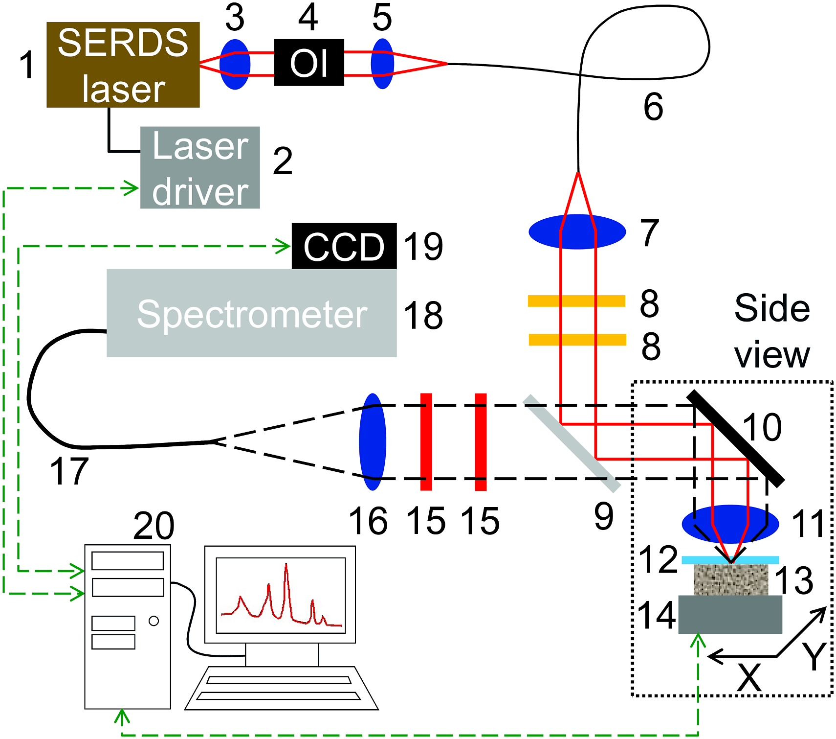

The backscattered light from the specimen is collected by (11) the same lens in 180° geometry and reflected by the (10) silver mirror. For improved blocking performance in case of highly scattering soil samples, a (9, 15) set of three Raman longpass filters (DI02-R785-25x36 and LP02-785RU-25, Semrock) rejects the elastically scattered radiation and anti-Stokes contributions while only the Raman Stokes scattered light (that is shifted to longer wavelengths with respect to the excitation laser light) passes through. By means of an (16) achromatic lens with a focal length of 60 mm and a diameter of 25.4 mm (Qioptiq), the light is then launched into an (17) optical fiber with a core diameter of 200 µm (Thorlabs) and transferred to the (18) spectrometer having an optical resolution of 4 cm⁻¹ (Tornado U1, Tornado Spectral Systems) with (19) attached charge-coupled device detector (CCD; MityCCD H10141, CriticalLink) thermo-electrically cooled down to −10 °C. In-house written software running on a computer (20) was used to set the laser and detector operation parameters, to facilitate recording of the Raman spectra and to control the movement of the motorized sample stage.

Sample Material and Reference Analyses

A set of 33 soil samples investigated in this study were collected at randomly selected locations from the topsoil layer (0–30 cm depth) across an agricultural field in northeast Germany (Latitude: 52.394316N; Longitude: 14.461156E) in 2017. The region was largely shaped by the Pleistocene glaciations and the Scandinavian inland ice sheet most of all by the Weichselian (115–12 ka) and the preceding Saalian glacial belt (150–130 ka).³⁰ The study field covers a considerably high within-field soil variability with respect to selected soil parameters. This can be seen exemplarily in Table I showing the descriptive statistics of laboratory reference data from our 33 specimens. The SOM content varies between 0.75% and 4.15% with a median at 1.4% while the total nitrogen content (N) ranges from 0.05% to 0.28% with a median of 0.09%. The pH values comprise a range from 5.3 (strongly acidic) to 7.3 (slightly alkaline) with a median at 6.6 (slightly acidic). According to the German soil classification system KA5,³¹ the soil texture (determined by the mass fractions of clay, silt, and sand) ranges from pure sand (class: Ss) to loamy sand (class: Sl) showing a dominance of loamy sand and silty sand (classes: Sl, Su).

Table I.

Descriptive statistics of selected soil parameters determined from 33 specimens collected from the study field.

	SOM (%)	N (%)	pH	Clay (%)	Silt (%)	Sand (%)
Average	1.65	0.10	6.5	6.7	19.6	73.7
Median	1.40	0.09	6.6	6.0	19.0	74.0
Minimum	0.75	0.05	5.3	2.0	5.0	48.0
Maximum	4.15	0.28	7.3	17.0	36.0	90.0
Range	3.40	0.23	2.0	15.0	31.0	42.0
Standard deviation	0.75	0.05	0.4	3.5	7.3	10.2

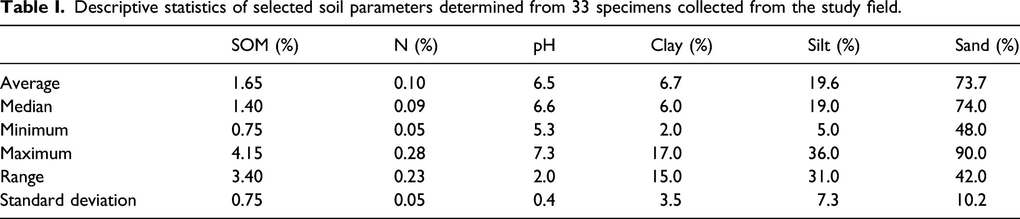
All 33 collected specimens were air-dried at room temperature and subsequently sieved to grain sizes smaller than 2 mm with a 2 mm mesh stainless steel sieve before further analysis. After homogenization, samples were divided into multiple subsets for laboratory reference analyses and for the SERDS experiments. Our study exemplarily focusses on the SOM and nitrogen content as selected important soil parameters and these were determined by the following standard laboratory methods. Elemental analysis with a Vario EL Cube (Elementar Analysensysteme GmbH) was applied according to Association of German Agricultural Investigation and Research Institutes method A 4.1.3.2 to determine soil organic carbon (SOC) content (as mass fraction in %). SOC content was then converted into SOM content using a conversion factor of 1.72 assuming that SOM contains approximately 58% of organic carbon.³² Total nitrogen content (as mass fraction in %) was determined using elemental analysis according to DIN ISO 13878 (1998-11) (dry combustion method).

Shifted Excitation Raman Difference Spectroscopy Measurement Conditions

For the SERDS experiments, the soil samples were transferred into small aluminum cups (diameter 30 mm) and covered with a 1 mm thick sapphire window. The specimens were mounted in a motorized x,y stage and probed at 100 positions in a 10 × 10-point grid pattern within an area of 1 cm². For an evaluation of the raster scan method, the distance between raster points (1.1 mm) and the overall covered raster area have been selected to take intrinsic soil variability at the millimeter scale into account. In an alternating operation mode between the two excitation wavelengths, at each spot 10 single Raman spectra with an accumulation time of 1 s were recorded. The optical power at the sample position was set to 20 mW to avoid potential sample heating and damage.

Spectral Processing and Data Analysis

For each probed spot, the recorded single Raman spectra were averaged resulting in two mean Raman spectra, one for each excitation wavelength. From these Raman spectra, the SERDS spectra were calculated according to an in-house developed algorithm implemented in Matlab (The MathWorks, Inc., USA). Initially, the difference of the two Raman spectra recorded at the slightly different wavelengths is calculated. To remove residual baseline modulations, this difference spectrum is fitted by a cubic spline function. The fitted function is then subtracted from the difference spectrum to achieve a baseline centered around zero. This is an important step to avoid the creation of spectral artifacts during the subsequent reconstruction procedure. In the next step, the baseline-corrected difference spectrum exhibiting a derivative-like spectral pattern is reconstructed by numerical integration to generate a Raman spectrum in conventional form. Following the numerical integration, the baseline of the reconstructed SERDS spectrum may not be exactly at zero. In the final step, an additional baseline correction of the reconstructed SERDS spectrum is therefore performed to achieve a straight horizontal baseline. The latter can be beneficial for further data processing, for example, intensity normalization.

For several measurement spots, very strong fluorescence interference in combination with spectrally narrow luminescence bands caused pronounced baseline distortions in the difference spectra that, in turn, led to artifacts in the reconstructed SERDS spectra. A similar issue with highly fluorescent/luminescent specimens has already been reported in another study conducted by our group.³³ To remove such outliers from the spectral data set, for each sample an empirically determined threshold of four times the mean intensity of the spectra recorded at the 100 different locations was calculated. On the one hand, this threshold allowed to reliably identify outliers but on the other hand it enabled to retain the natural variability of Raman signal intensities recorded on heterogenous soil. Individual spectra with artifacts exceeding the threshold value were then discarded. On rare occasions, fluorescence was so intense to cause the CCD detector to saturate and these spectra were removed as well. Overall, on average, seven measurement spots out of 100 were removed for each investigated sample. To consider the inherent soil heterogeneity, the remaining spectra were averaged before further processing to achieve one representative mean spectrum for each specimen.

The spectral range from 340–1640 cm⁻¹ has been selected for the calculation of partial least squares (PLS) regression models in our case as it contains characteristic Raman signals of the majority of mineral and organic soil components. Prior to multivariate regression, SERDS spectra were truncated to this range and normalized to the intensity of the 418 cm⁻¹ Raman band originating from the sapphire window. For the PLS regression of the SERDS data against the determined reference laboratory values for the SOM and nitrogen content, the Matlab function “plsregress” based on the SIMPLS algorithm³⁴ and included in the Statistics and Machine Learning Toolbox was applied. Due to the relatively small number of 33 samples, leave-one-out cross validation was selected as suitable cross validation method.

Results and Discussion

Spatial Resolution of Shifted Excitation Raman Difference Spectroscopy Setup

Prior to soil investigations, an important point is to evaluate the spatial resolution of the SERDS setup in axial and lateral direction. Using a silicon sample and translating it through the laser focus along the beam propagation direction is a common practice to determine the depth of focus of a Raman setup.³⁵ In this way, SERDS spectra were recorded covering a total axial range of 6 mm around the focal position. The determined net intensities of the prominent silicon Raman band at 520 cm⁻¹ were normalized to their maximum and are displayed as black open diamond symbols in Fig. 2a. It is well known from theoretical considerations that such intensity profiles represent a Lorentzian distribution.^35,36 A corresponding fit of the experimental data is displayed as red solid line. The results show that the depth of focus where the intensity drops to half of the maximum value (full width at half-maximum, FWHM) amounts to 760 µm.

Figure 2.

Normalized SERDS net intensities of silicon Raman signal at 520 cm⁻¹. Dependence of axial sample position (black diamonds) with fitted Lorentzian function (red curve) (a) and dependence of lateral sample position (black squares) with fitted Gaussian error function (blue curve), blue dashed lines indicate transition width (b).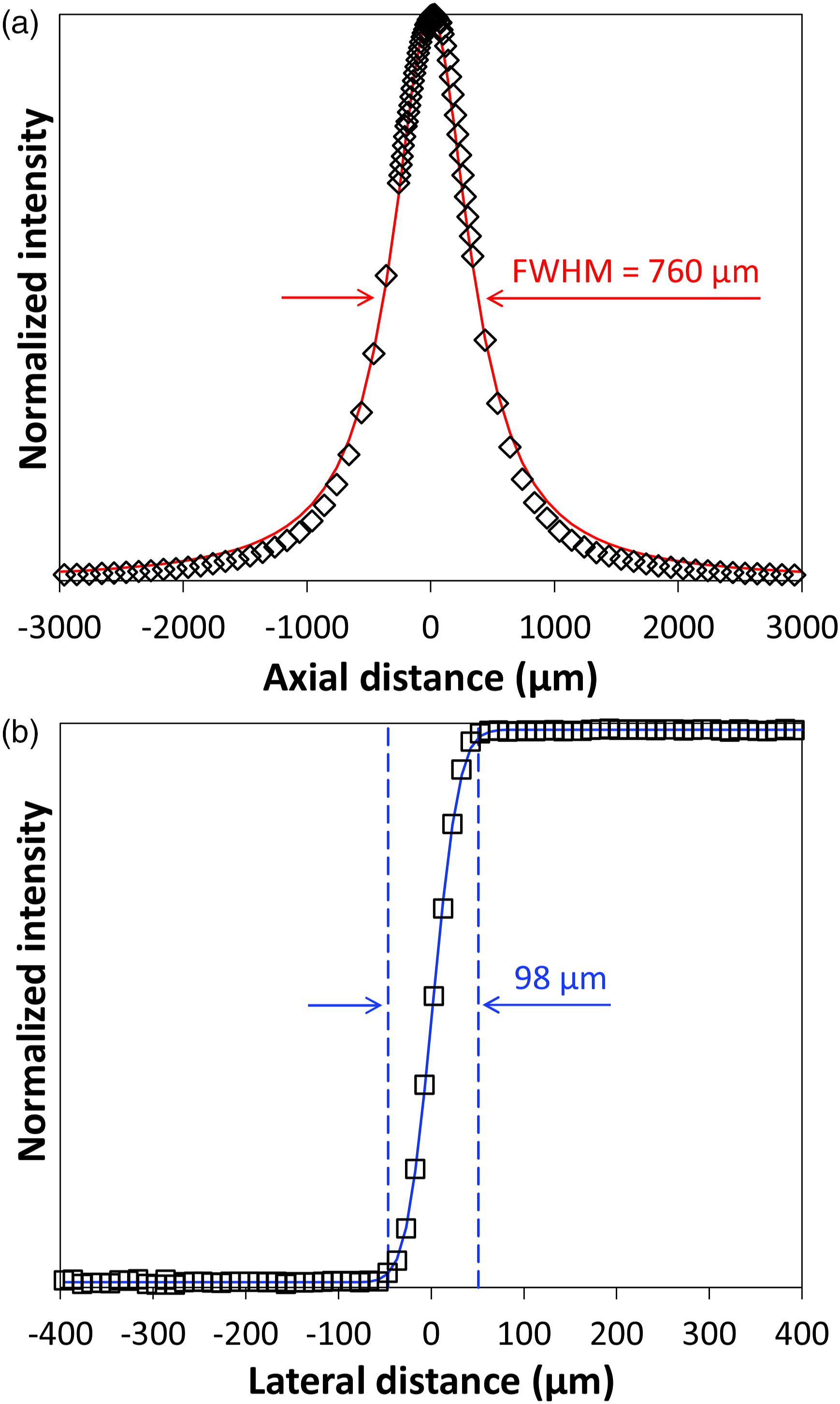

To assess the lateral resolution of the experimental setup, the edge of the silicon sample has been translated perpendicular towards the beam propagation direction within the focal plane. This common procedure of moving the laser beam across a well-defined edge has been described in the literature previously.^37,38 SERDS spectra were recorded comprising a total lateral distance of 800 µm around the edge of the silicon specimen. Figure 2b displays the calculated net intensities of the 520 cm⁻¹ silicon Raman band normalized to their maximum as black open square symbols. The experimental data was then fitted using a Gaussian error function³⁸ that is displayed as solid blue line. Subsequently, the transition width defined as four times the width parameter of the Gaussian profile can be used to determine the lateral resolution. Its value amounts to 98 µm and is close to the estimated laser spot size of approximately 90 µm.

Our previous study has shown that in a confocal Raman microscopic geometry, there is a need for active focus adjustment during the measurement when investigating soil specimens.¹⁷ This is due to the presence of a surface topology in combination with very small depths of focus in the range of a few micrometers only. In the present investigation, the soil samples have been prepared according to standard laboratory procedures to contain particle sizes of up to 2 mm. It should be noted that the actual surface roughness during the experiments will however be much smaller than the maximum particle size. A mixture of small and large particles will be present in the samples and by pressing the plane sapphire window on top of the soil specimens, a relatively flat surface structure can be realized as confirmed by visual inspection. The residual surface roughness due to the intrinsic soil structure is therefore not an issue as the experimental setup provides a sufficiently large depth of focus to compensate for such variations.

Raman and Shifted Excitation Raman Difference Spectroscopy Spectra of Soil

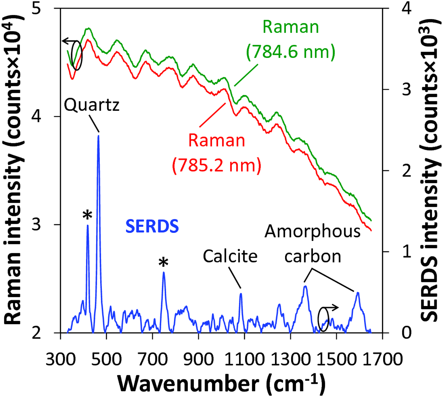
The averaged 100 single Raman spectra recorded for each excitation wavelength from 10 measurement spots along a distance of 10 mm are exemplarily displayed in Fig. 3 (top curves) for one selected soil sample. It becomes obvious that due to strong fluorescence interference, no Raman signals of soil constituents can be observed. Application of SERDS according to the procedure described above, however, can reveal the previously masked Raman spectroscopic information. The reconstructed SERDS spectrum (bottom curve in Fig. 3) enables the identification of the strongest characteristic Raman bands within the presented inspection range. Contributions at 418 cm⁻¹ and 750 cm⁻¹ (marked by asterisks) arise from the sapphire window used to cover the soil sample.³⁹ Furthermore, Raman signals of the mineral components quartz⁴⁰ (SiO₂) at 465 cm⁻¹ and calcite⁴¹ (CaCO₃) at 1083 cm⁻¹ can be identified. The broad Raman signals around 1360 cm⁻¹ and 1590 cm⁻¹ can be attributed to the D-band and G-band of amorphous carbon, respectively.^40,42 In this way, SERDS could successfully be applied to recover Raman spectroscopic information from strong fluorescence interference in soil thus enabling the identification of selected mineral soil constituents as well as amorphous carbon.

Figure 3.

Average of 100 Raman spectra (top curves) excited at 785.2 nm and 784.6 nm, and corresponding reconstructed SERDS spectrum (bottom curve) obtained from 10 individual measurement positions along a distance of 10 mm of a selected soil sample. The Raman spectrum excited at 784.6 nm is vertically offset by 1000 counts for clarity. The asterisks on the SERDS spectrum indicate characteristic Raman signals of the sapphire window that is used to cover the soil sample.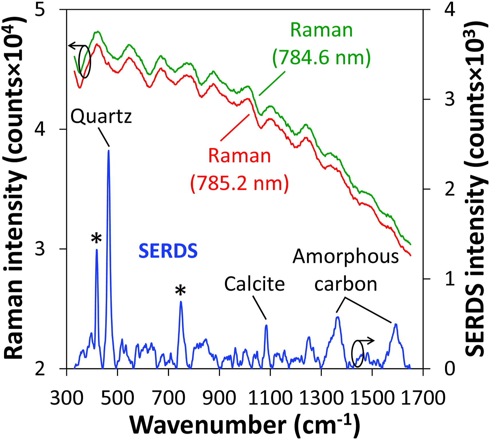

For comparison, Supplemental Figure S1 (Supplemental Material) shows a plot of the Raman spectrum excited at 785.2 nm after polynomial background correction⁴³ (seventh-order polynomial function, 50 iterations) together with the SERDS spectrum displayed in Fig. 3. It becomes obvious that the polynomial procedure is unable to adequately separate the characteristic Raman signals of soil constituents from background interferences. Here, only the major quartz Raman signal at 465 cm⁻¹ is barely visible while the other Raman signals identifiable in the SERDS spectrum are completely masked. This example highlights the capability of SERDS to properly address interfering contribution in the Raman spectra leading to an efficient extraction of the Raman spectroscopic information from the soil sample under investigation.

Assessment of Soil Heterogeneity

It is well known that soil samples show an intrinsic spatial heterogeneity at multiple length scales. In our previous study using Raman microscopy with an excitation spot size in the order of 1 µm on a soil microaggregate with <1 mm diameter, we have shown that there exists a spatial variability of soil components on the micrometer (μm) scale.¹⁷ In the present investigation, this variability has been addressed by applying a larger excitation spot size of ca. 90 µm. Furthermore, to account for spatial variations occurring on the millimeter (mm) scale, a raster of 100 points, comprised of a 10 × 10-point grid covering a total area of 1 cm², has been scanned for all specimens. Based on visual inspection of the SERDS spectra recorded at each measurement spot and comparison with the characteristic Raman signals identified in the SERDS spectrum displayed in Fig. 3, a coarse assessment has been made for the presence of selected soil constituents. Figure 4 shows the resulting plots for one selected soil specimen indicating the detection of quartz, calcite, and amorphous carbon at various measurement spots.

Figure 4.

Plots showing the spatial distribution of the soil constituents (a) quartz, (b) calcite, and (c) amorphous carbon for one selected soil specimen. Colored squares (red, green, and blue) indicate measurement spots where the corresponding substance has been identified by visual inspection of the SERDS spectra and comparison with the characteristic Raman signals indicated in the SERDS spectrum displayed in Figure 3.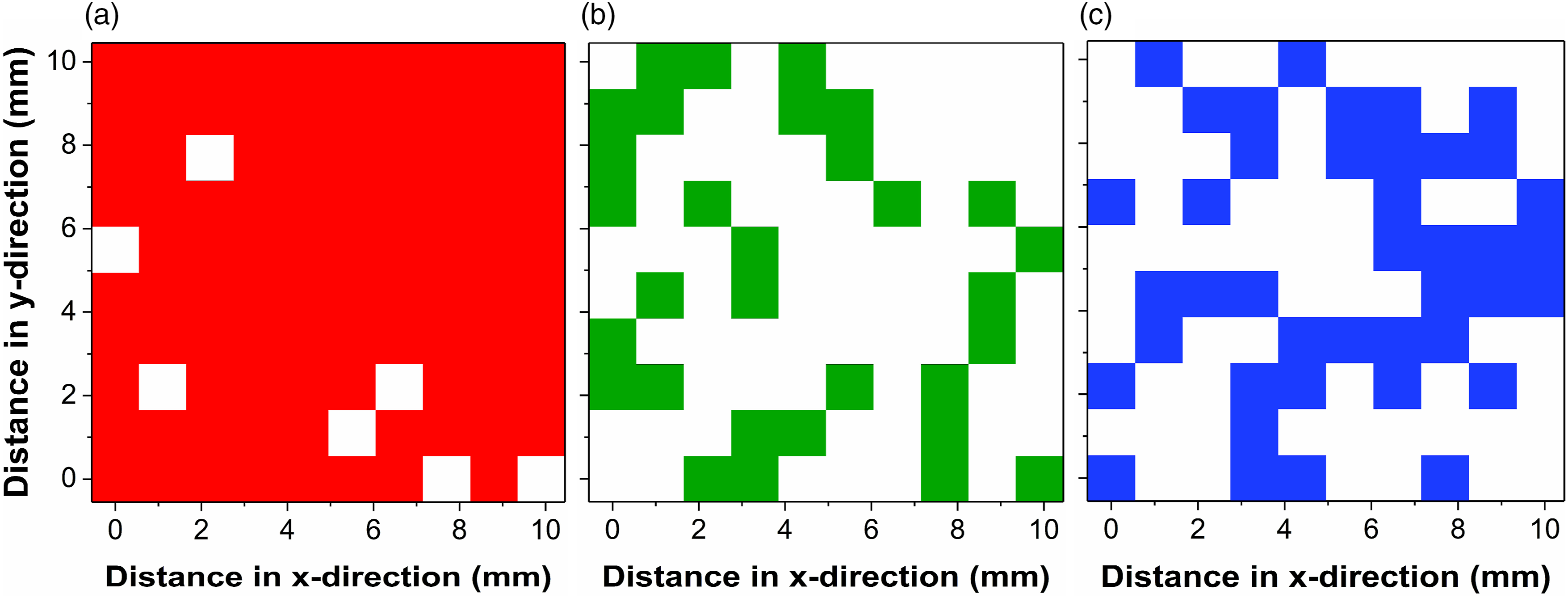

Within the selected sample, quartz as one of the most abundant soil constituents could be identified at 93 out of 100 measurement spots (see Fig. 4a). Beside its high concentration in the samples, detection of quartz is eased by the strong and relatively isolated major Raman signal at 465 cm⁻¹. For calcite, the spatial heterogeneity is more pronounced as depicted in Fig. 4b. Identification based on the main Raman signal at 1083 cm⁻¹ was possible at 31 spots in total. The spatial distribution is characterized by numerous clusters comprising up to six adjacent measurement spots, whereas there are also extended areas without the presence of calcite. The spatial distribution for amorphous carbon as selected organic constituent is depicted in Fig. 4c. It should be noted that, based on relatively noisy single spot spectra, the identification of the rather broad Raman signals at 1360 cm⁻¹ and 1590 cm⁻¹ can be challenging. Nevertheless, the applied visual inspection method allows for a rough estimate of the spatial distribution of amorphous carbon, indicating its presence at 41 out of 100 measurement spots. The distribution shows a couple of isolated spots but is generally dominated by larger clusters of adjacent measurement positions. The plots presented show that a pronounced spatial variability of the content of selected soil components is present on a millimeter-sized scale. In our study, we have addressed the issue of soil heterogeneity at this length scale by averaging the 100 SERDS spectra recorded from within an area of ∼1 cm² to obtain more representative spectra of the investigated soil samples.

In Fig. 5, these averaged SERDS spectra obtained from three different soil samples are presented. For better visualization, the spectra were normalized to the intensity of the sapphire Raman signal at 418 cm⁻¹ and vertically offset. In contrast to the average spectrum from 10 single measurement spots displayed in Fig. 3, the mean SERDS spectra of all 100 probed locations now allow for the identification of a smaller contribution from the sapphire window at 578 cm⁻¹ as well.³⁹ Furthermore, characteristic Raman signals of the additional mineral soil components feldspar⁴⁴ at 512 cm⁻¹ and anatase (TiO₂)⁴⁵ at 634 cm⁻¹ can be identified. Due to inherent soil heterogeneity, as expected, the Raman signal intensities of the indicated constituents exhibit pronounced variations with individual components even being virtually absent in some cases.

Figure 5.

Averaged SERDS spectra of three selected soil samples. Vertical dashed lines highlight the Raman signal positions of identified soil constituents and asterisks indicate Raman signals of the sapphire window. Spectra are normalized to the intensity of the sapphire signal at 418 cm⁻¹ and are vertically offset for clarity.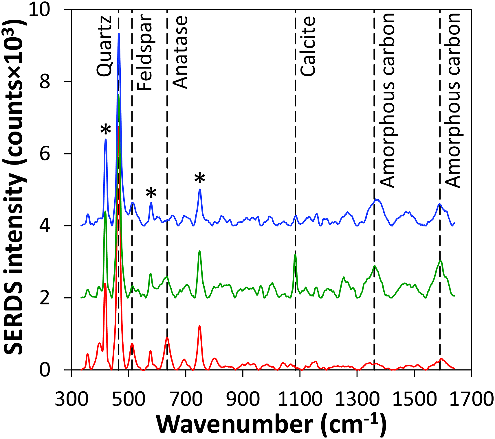

For a further assessment of the variations of individual soil components between the investigated 33 specimens, the respective Raman signal intensities of quartz (465 cm⁻¹), feldspar (512 cm⁻¹), anatase (634 cm⁻¹), calcite (1083 cm⁻¹), and amorphous carbon (1360 cm⁻¹) have been calculated from the SERDS spectra (average of three points around signal maximum). Figure 6 presents the corresponding intensities that have been normalized to their respective maximum and were vertically offset for clarity. As a measure to assess the distribution of individual components, the median was calculated. This statistical value splits the data in such a way that half of the data is above it and half of the data is below it. In our case, the smaller the median, the more heterogenous the distribution of the corresponding soil component can be considered. For the two mineral components quartz and feldspar the median amounts to 58% and 56% of their maximum intensity, respectively. The frequent occurrence of these two constituents is not surprising as they are among the most abundant materials within various soils.⁴⁶ In the case of anatase and carbon, the medians are 16% and 20% of the maximum intensity, respectively, indicating a pronounced heterogenous distribution among the 33 samples. The strongest variation is present for calcite with a median of only 3% of the corresponding maximum value. Here, only very few specimens contain medium and high relative intensities.

Figure 6.

Shifted excitation Raman difference spectroscopy signal intensities of quartz (at 465 cm⁻¹), feldspar (at 512 cm⁻¹), anatase (at 634 cm⁻¹), calcite (at 1083 cm⁻¹), and amorphous carbon (at 1360 cm⁻¹) plotted versus sample number. Values are normalized to their respective maximum and vertically offset for clarity.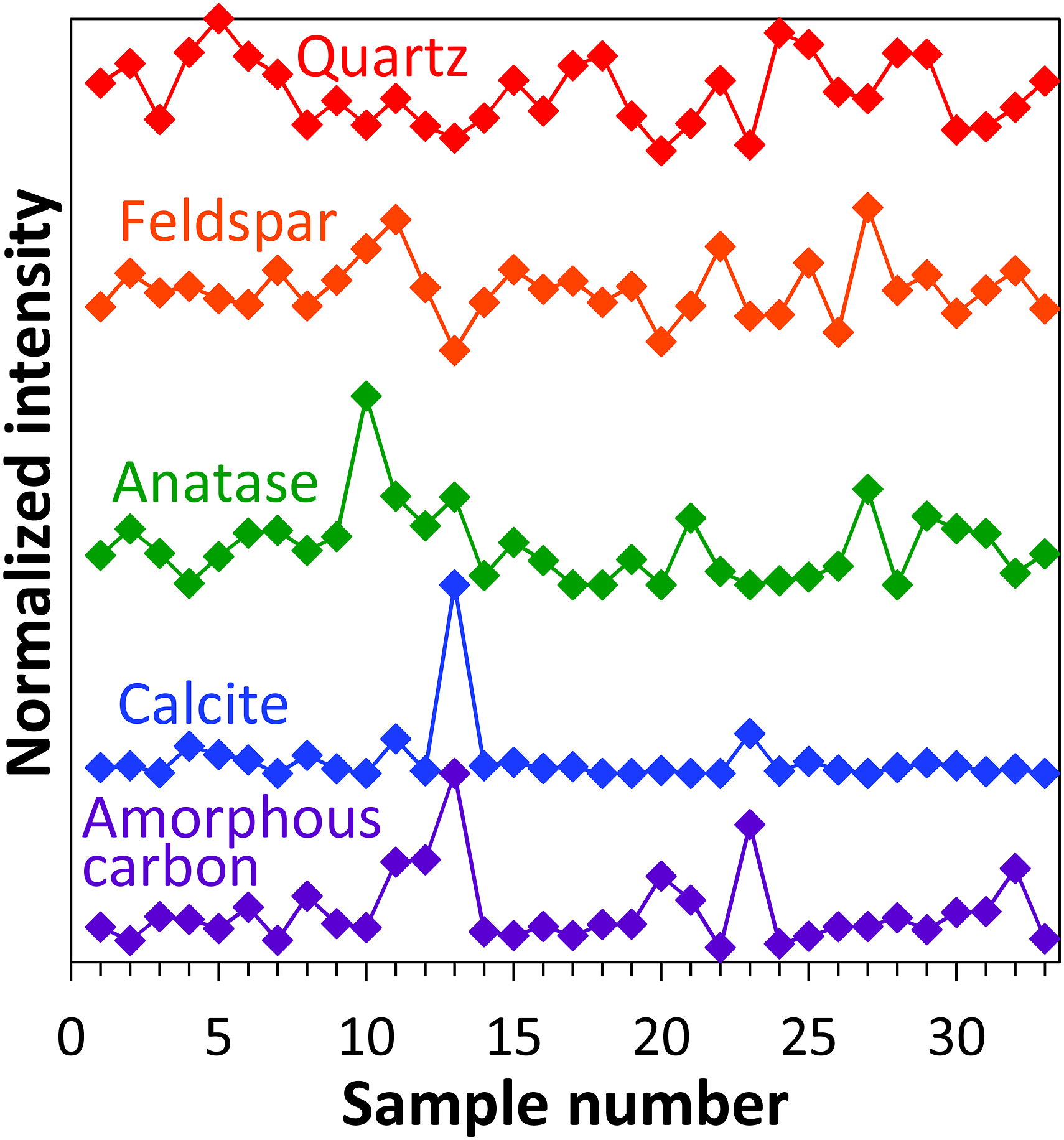

Visual inspection of Fig. 6 shows that some of the samples with high calcite content also contain larger amounts of amorphous carbon. Closer inspection reveals that there exists a positive correlation between the intensities of both soil constituents with a value of determination of R² = 0.56. This observation is in accordance with the literature where a coincidence between organic matter and calcite has been reported for certain soil types.²² In the next step, using multivariate analysis, the SERDS spectra will be correlated with the SOM and nitrogen contents as determined by laboratory reference analyses to assess whether the spectroscopic data can be used to determine these key soil parameters.

Partial Least Squares Regression

Initially, averaged SERDS data of all 33 investigated soil samples have been subjected to PLS regression analysis aiming for the prediction of the SOM content. An important initial step is the proper selection of the number of PLS components included into the regression model. A commonly applied strategy for the identification of a suitable number of PLS components is to calculate the model root mean square error of cross validation (RMSECV) as a function of the number of components and to determine its minimum. In this way, a number of three components have been identified and PLS regression of the recorded SERDS spectra (normalized to the intensity of the 418 cm⁻¹ sapphire Raman band) against the reference SOM values determined by conventional laboratory analysis was performed within the selected spectral range from 340 to 1640 cm⁻¹.

A plot of the SOM contents predicted from the SERDS data in dependence of the corresponding contents determined by laboratory reference analysis is given in Fig. 7. Here, a very good linear correlation between predicted and measured SOM content with a coefficient of determination of R² = 0.82 can be realized. A further measure to assess the performance of the prediction is the slope of the linear fit (dashed line). As the model should directly predict the measured value itself, that is, without a scaling factor, the slope will ideally be 1.0. Here, the slope amounts to 0.97 and is thus very close to the ideal 1:1 relation (solid line) between predicted and measured SOM content. As a rough visualization of the model accuracy, error bars with the length of RMSECV (0.41% SOM content) have been added to the data points.

Figure 7.

Soil organic matter content predicted from SERDS spectra of 33 soil samples using PLS regression model with three components plotted in dependence of corresponding SOM content measured by laboratory reference analysis (dashed line: linear fit, solid line: 1:1 dependence).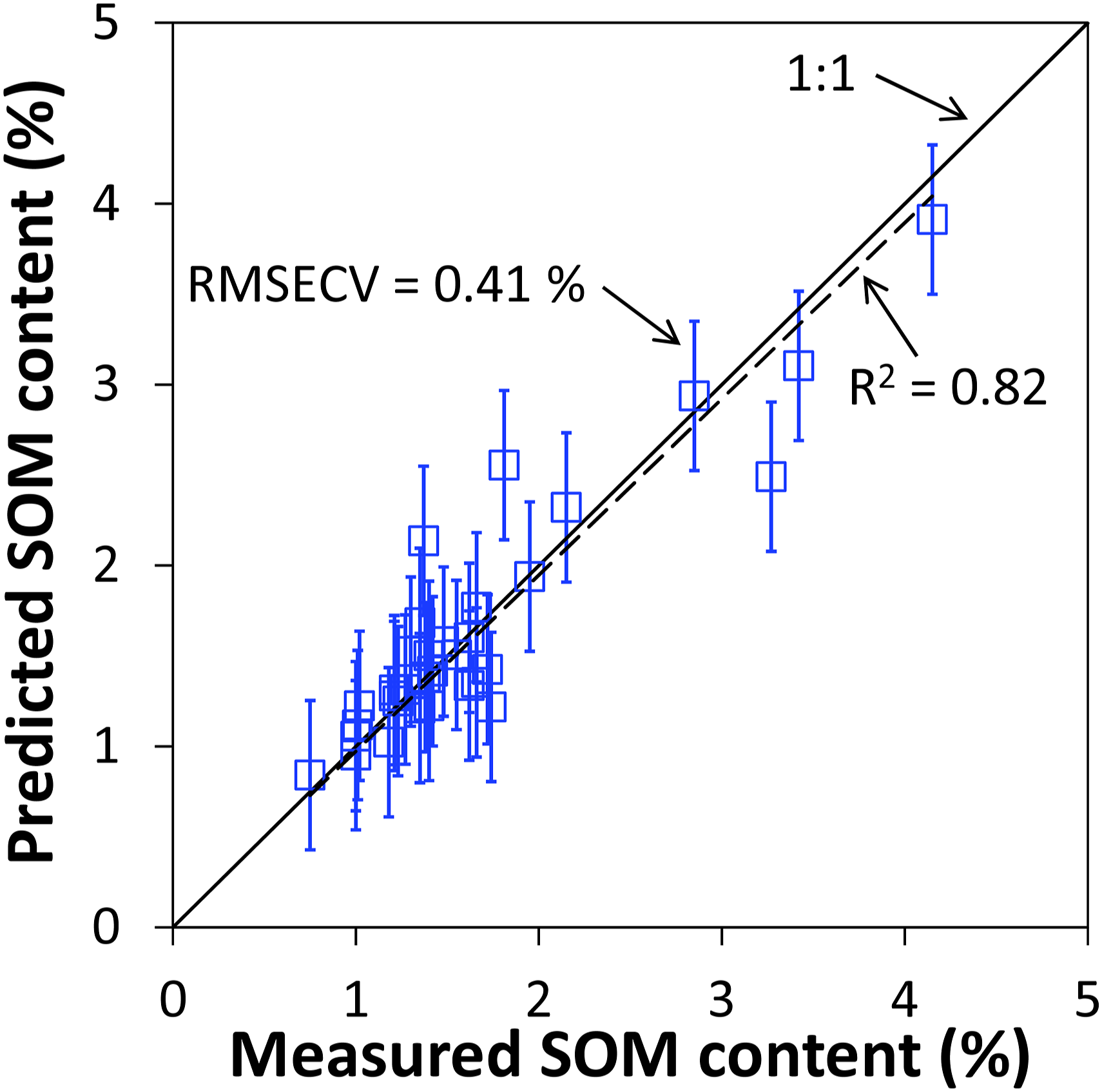

Besides the R² value and the RMSECV, a further commonly used measure to evaluate the model quality is the ratio of percentage deviation (RPD).⁴⁷ This value is calculated by dividing the standard deviation of the laboratory reference values (0.75% in our case) by the RMSECV of the PLS regression model and amounts to 1.81. Based on the classification given by Viscarra Rossel et al.,⁴⁷ RPD values between 1.8 and 2.0 indicate a sufficient model performance to enable quantitative predictions. In this way, the molecule-specific information derived from the SERDS data is suitable for the quantitative assessment of the SOM content.

During the regression, the PLS algorithm identifies suitable spectral channels that can be used to predict the SOM content from the spectroscopic data. To assess these spectral characteristics, a plot of the regression coefficients for the SOM content in the investigated wavenumber range is presented in Fig. 8. Overall, a couple of prominent signals can be identified. High coefficients can be found at spectral positions related to contributions coming from calcite at 1083 cm⁻¹ and amorphous carbon at 1360 cm⁻¹ and 1590 cm⁻¹. In contrast, low coefficients can be observed at spectral positions related to contributions originating form quartz at 465 cm⁻¹ and feldspar at 512 cm⁻¹. As SOM is directly related to organic carbon content, the presence of prominent signals at characteristic Raman wavenumbers of amorphous carbon is reasonable. The appearance of the calcite signal could be explained by the above-mentioned correlation between calcite and carbon content. In contrast, quartz and feldspar as some of the most abundant soil constituents do not play a significant role in SOM content prediction.

Figure 8.

Regression coefficients of PLS model with three components used to predict SOM content from SERDS spectra. Vertical dashed lines indicate Raman band positions of identified soil constituents.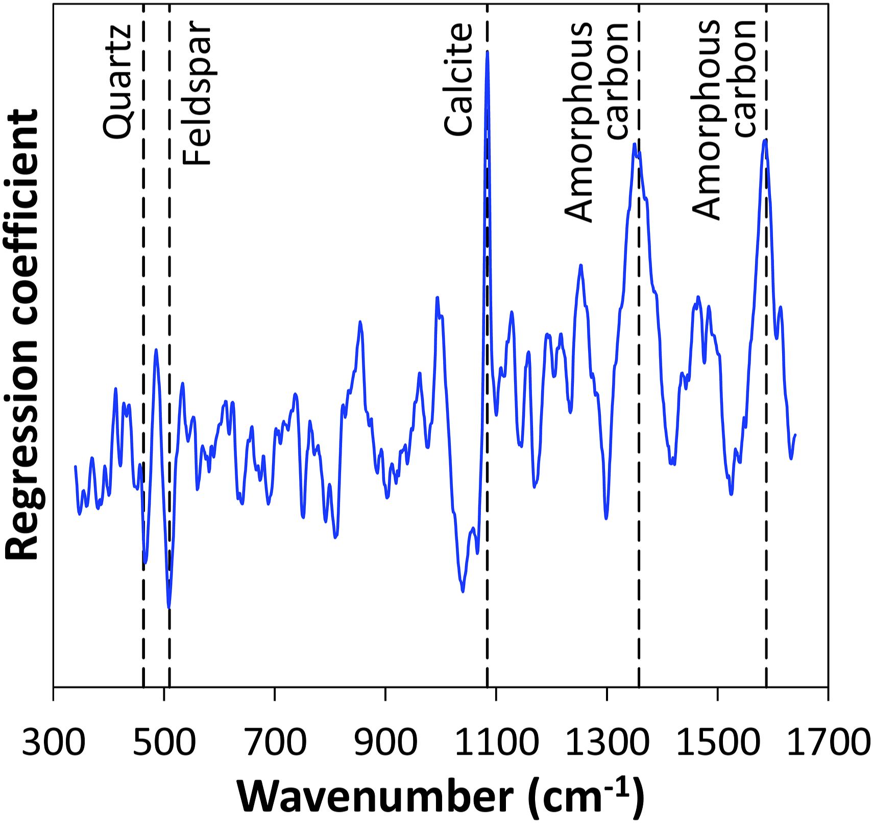

It is noteworthy that a similar investigation on Chinese farmland soils applying conventional Raman spectroscopy (i.e., without using SERDS) at 785 nm excitation wavelength has been conducted recently.⁴⁸ As in our study, the characteristic Raman fingerprint of the soil samples was superimposed by strong fluorescence interference. The authors employed a mathematical background correction and correlated their spectra with laboratory values for SOM content using PLS regression. Based on a number of 200 spectra (150 samples for calibration set, 50 samples for validation set), their model using seven factors achieved values of R² = 0.74 and root mean squared error of prediction RMSEP = 0.82%. However, no PLS regression coefficients are given in this case to examine the underlying spectral characteristics responsible for the obtained prediction model.

Within their 200 samples, the range of investigated SOM contents (0.57–9.70%) is about 2.7 times larger than the SOM range present in our 33 specimens (0.75–4.15%). Despite the reduced range of investigated SOM contents and the much smaller number of specimens, our investigation shows better performance for several important model indicators (higher R², lower RMSECV and smaller number of factors required). The most likely cause for this behavior is the capability of SERDS for the efficient extraction of the Raman spectroscopic information from disturbing interferences such as fluorescence. As an example, our previous investigation on soil has shown that a ten-fold improvement in the signal-to-background noise ratio can be achieved by applying SERDS.¹⁷ Additionally, in the study on Chinese farmland soils, the authors identified fluorescence as a major obstacle to obtain high quality soil Raman spectra.⁴⁸ Due to the effective fluorescence removal applied in our investigation, the input quality of the SERDS data for PLS regression is expected to be superior to conventional Raman data thus leading to improved model performance.

In the case of nitrogen, a very good linear correlation between predicted values from the SERDS data and the measured nitrogen content by laboratory reference analysis could be realized using PLS regression (R² = 0.86, RMSECV = 0.026%, model with three components). The regression coefficients of the PLS model show a nearly identical spectral pattern compared to the one obtained for the SOM content that is displayed in Fig. 8. It is, however, important to note that the achieved correlation for the soil nitrogen content is only an indirect correlation rather than being based on direct Raman spectroscopic information. In the SERDS spectra as well as in the PLS regression coefficients, no evidence was found indicating the presence of nitrogen-containing compounds, most likely due to their low concentration within our investigated soil samples (0.05–0.28% as determined by laboratory reference analysis). The explanation for the very good prediction of the nitrogen content can be found when considering the soil composition. There exists a very strong positive correlation with R² = 0.97 between the reference values for SOM and nitrogen content as determined by conventional laboratory analyses. From a soil science perspective this is not surprising as nitrogen in the topsoil layers is naturally present to more than 90% in an organic form.⁴⁹ Consequently, the contents of nitrogen and SOM within topsoil are usually positively correlated.

The results obtained demonstrate that SERDS spectra acquired on agricultural soil samples can be used for determination of the SOM content as well as for the identification of other soil constituents. Laboratory investigations on air-dried and sieved samples have shown the potential of SERDS for qualitative and quantitative soil analysis. Sample preprocessing was minimal in this case and done according to standard sample preparation procedures in soil science. Raman spectroscopy, however, does not require dry samples as interference from water is only minimal in the investigated Raman fingerprint range. Thus, in the future, potentially even in situ investigations using portable SERDS instrumentation²⁷ on agricultural fields seem feasible for screening of selected soil parameters. With respect to such practical applications of SERDS in agriculture, an appropriate way to consider the soil spatial heterogeneity on-site to obtain representative SERDS spectra suitable for quantitative analysis is still under investigation. Further research is directed towards the identification and confirmation of a suitable sampling strategy, including the assessment of the number of required measurement spots for each probed site.

Conclusion

This study successfully demonstrated that SERDS at 785 nm excitation wavelength can effectively recover the characteristic molecular fingerprint of selected inorganic (quartz, feldspar, anatase, and calcite) and organic (amorphous carbon) components within soil from intense fluorescence interference. Soil spatial variability at the millimeter scale has been addressed by using a raster scan with 100 individual measurement spots per sample. Results obtained on a set of 33 soil samples collected from an agricultural field show that the molecule-specific spectroscopic information provided can be used for the prediction of the SOM content as important soil parameter (R² = 0.82, RMSECV = 0.41%). These outcomes highlight the large potential of SERDS as a promising tool for soil analysis in precision agriculture paving the way for efficient soil nutrient management.

Supplemental Material

sj-pdf-1-asp-10.1177_00037028211064907 – Supplemental Material for Determination of Soil Constituents Using Shifted Excitation Raman Difference Spectroscopy

Supplemental Material, sj-pdf-1-asp-10.1177_00037028211064907 for Determination of Soil Constituents Using Shifted Excitation Raman Difference Spectroscopy by Kay Sowoidnich, Sebastian Vogel, Martin Maiwald, and Bernd Sumpf in Applied Spectroscopy

Footnotes

Acknowledgments

This work is realized within the project RaMBo (Raman-Messsystem zur ortsspezifischen Bodenanalytik) within the consortium I4S (Intelligence for Soil) in the frame of the funding measure BonaRes (Soil as a Sustainable Resource for the Bioeconomy). We would like to thank all involved colleagues from I4S (https://i4s.atb-potsdam.de/en/project) and the pH-BB project () for sample collection and preparation, the landowner Golo Philipp for access to the agricultural field and the external laboratories for conducting the reference analyses of the soil samples. We are particularly grateful to Maria Krichler (Ferdinand-Braun-Institut gGmbH, Leibniz-Institut für Höchstfrequenztechnik) for developing the software to control the experimental setup.

Declaration of Conflicting Interests

The author(s) declared no potential conflicts of interest with respect to the research, authorship, and/or publication of this article.

Funding

The author(s) disclosed receipt of the following financial support for the research, authorship, and/or publication of this article: This work was supported by the Federal Ministry of Education and Research (BMBF) [grant number 031B0513C].

ORCID iD

Kay Sowoidnich

Martin Maiwald

Supplemental Material

All supplemental material mentioned in the text is available in the online version of the journal.

References

Gebbers

Adamchuk

V.I.

. “Precision Agriculture and Food Security”. Science. 2010. 327(5967): 828‐831. doi:10.1126/science.1183899.

Bhakta

Phadikar

Majumder

. “State-of-the-Art Technologies in Precision Agriculture: A Systematic Review”. J. Sci. Food Agric. 2019. 99(11): 4878‐4888. doi:10.1002/jsfa.9693.

Bongiovanni

Lowenberg-Deboer

. “Precision Agriculture and Sustainability”. Precis. Agric. 2004. 5(4): 359‐387. doi:10.1023/B:PRAG.0000040806.39604.aa.

Leenen

Welp

Gebbers

Pätzold

. “Rapid Determination of Lime Requirement by Mid-Infrared Spectroscopy: A Promising Approach for Precision Agriculture”. J. Plant Nutr. Soil Sci. 2019. 182(6): 953‐963. doi:10.1002/jpln.201800670.

Nanni

M.R.

Povh

F.P.

Demattê

J.A.M.

, et al. “Optimum Size in Grid Soil Sampling for Variable Rate Application in Site-Specific Management”. Sci. Agric. 2011. 68(3): 386‐392. doi:10.1590/s0103-90162011000300017.

Pätzold

Mertens

F.M.

Bornemann

, et al. “Soil Heterogeneity at the Field Scale: A Challenge for Precision Crop Protection”. Precis. Agric. 2008. 9(6): 367‐390. doi:10.1007/s11119-008-9077-x.

Stoyan

De-Polli

Böhm

Robertson

G.P.

Paul

E.A.

. “Spatial Heterogeneity of Soil Respiration and Related Properties at the Plant Scale”. Plant Soil. 2000. 222(1–2): 203‐214. doi:10.1023/a:1004757405147.

Rinot

Levy

G.J.

Steinberger

Svoray

Eshel

. “Soil Health Assessment: A Critical Review of Current Methodologies and a Proposed New Approach”. Sci. Total Environ. 2019. 648: 1484‐1491. doi:10.1016/j.scitotenv.2018.08.259.

Viscarra Rossel

R.A.

McBratney

A.B.

. “Soil Chemical Analytical Accuracy and Costs: Implications from Precision Agriculture”. Aust. J. Exp. Agric. 1998. 38(7): 765‐775. doi:10.1071/EA97158.

10.

Büchele

Chao

Ostermann

Leenen

Bald

. “Multivariate Chemometrics as a Key Tool for Prediction of K and Fe in a Diverse German Agricultural Soil-Set using EDXRF”. Sci. Rep. 2019. 9: 17588. doi:10.1038/s41598-019-53426-5.

11.

Rühlmann

Büchele

Ostermann

Bald

Schmid

. “Challenges in the Quantification of Nutrients in Soils using Laser-Induced Breakdown Spectroscopy: A Case Study with Calcium”. Spectrochim. Acta B. 2018. 146: 115‐121. doi:10.1016/j.sab.2018.05.003.

12.

Riebe

Erler

Brinkmann

, et al. “Comparison of Calibration Approaches in Laser-Induced Breakdown Spectroscopy for Proximal Soil Sensing in Precision Agriculture”. Sensors. 2019. 19: 5244. doi:10.3390/s19235244.

13.

Erler

Riebe

Beitz

Löhmannsröben

H.-G.

Gebbers

. “Soil Nutrient Detection for Precision Agriculture using Handheld Laser-Induced Breakdown Spectroscopy (LIBS) and Multivariate Regression Methods (PLSR, Lasso and GPR)”. Sensors. 2020. 20: 418. doi:10.46770/AS.2020.03.003.

14.

Heggemann

Welp

Amelung

et al. “Proximal Gamma-Ray Spectrometry for Site-Independent In Situ Prediction of Soil Texture on Ten Heterogeneous Fields in Germany Using Support Vector Machines”. Soil Tillage Res. 2017. 168: 99‐109. doi:10.1016/j.still.2016.10.008.

15.

Pätzold

Leenen

Heggemann

T.W.

. “Proximal Mobile Gamma Spectrometry as Tool for Precision Farming and Field Experimentation”. Soil Syst. 2020. 4: 31. doi:10.3390/soilsystems4020031.

16.

Heil

Schmidhalter

. “An Evaluation of Different NIR-Spectral Pre-Treatments to Derive the Soil Parameters C and N of a Humus-Clay-Rich Soil”. Sensors. 2021. 21: 1423. doi:10.3390/s21041423.

17.

Theurer

L.S.

Maiwald

Sumpf

. “Shifted Excitation Raman Difference Spectroscopy: A Promising Tool for the Investigation of Soil”. Eur. J. Soil Sci. 2021. 72(1): 120‐124. doi:10.1111/ejss.12928.

18.

Janik

L.J.

Soriano-Disla

J.M.

Forrester

S.T.

McLaughlin

M.J.

. “Moisture Effects on Diffuse Reflection Infrared Spectra of Contrasting Minerals and Soils: A Mechanistic Interpretation”. Vib. Spectrosc. 2016. 86: 244–252. doi:10.1016/j.vibspec.2016.07.005.

19.

Carrero

J.A.

Goienaga

Olivares

, et al. “Raman Spectroscopy assisted with XRF and Chemical Simulation to Assess the Synergic Impacts of Guardrails and Traffic Pollutants on Urban Soils”. J. Raman Spectrosc. 2012. 43(10): 1498‐1503. doi:10.1002/jrs.4089.

20.

Edwards

Munshi

Scowen

Surtees

Swindles

G.T.

. “Development of Oxidative Sample Preparation for the Analysis of Forensic Soil Samples with Near-IR Raman Spectroscopy”. J. Raman Spectrosc. 2012. 43(2): 323‐325. doi:10.1002/jrs.3031.

21.

Vogel

Adam

Sekine

, et al. “Determination of Phosphorus Fertilizer Soil Reactions by Raman and Synchrotron Infrared Microspectroscopy”. Appl. Spectrosc. 2013. 67(10): 1165‐1170. doi:10.1366/13-07056.

22.

Vogel

Ramsteiner

Sekine

Doolette

Adam

. “Characterization of Phosphorus Compounds in Soils by Deep Ultraviolet (DUV) Raman Microspectroscopy”. J. Raman Spectrosc. 2017. 48(6): 867‐871. doi:10.1002/jrs.5115.

23.

Shreve

A.P.

Cherepy

N.J.

Mathies

R.A.

. “Effective Rejection of Fluorescence Interference in Raman Spectroscopy Using a Shifted Excitation Difference Technique”. Appl. Spectrosc. 1992. 46(4): 707–711. doi:10.1366/0003702924125122.

24.

Zhao

Carrabba

M.M.

Allen

F.S.

. “Automated Fluorescence Rejection Using Shifted Excitation Raman Difference Spectroscopy”. Appl. Spectrosc. 2002. 56(7): 834‐845. doi:10.1366/000370202760171491.

25.

Maiwald

Sumpf

Tränkle

. “Rapid and Adjustable Shifted Excitation Raman Difference Spectroscopy Using a Dual-Wavelength Diode Laser at 785 nm”. J. Raman Spectrosc. 2018. 49(11): 1765–1775. doi:10.1002/jrs.5456.

26.

Maiwald

Müller

Sumpf

Erbert

Tränkle

. “Capability of Shifted Excitation Raman Difference Spectroscopy Under Ambient Daylight”. Appl. Opt. 2015. 54(17): 5520. doi:10.1364/ao.54.005520.

27.

Maiwald

Müller

Sumpf

Tränkle

. “A Portable Shifted Excitation Raman Difference Spectroscopy System: Device and Field Demonstration”. J. Raman Spectrosc. 2016. 47(10): 1180‐1184. doi:10.1002/jrs.4953.

28.

Sumpf

Maiwald

Müller

, et al. “Comparison of Two Concepts for Dual-Wavelength DBR Ridge Waveguide Diode Lasers at 785 nm Suitable for Shifted Excitation Raman Difference Spectroscopy”. Appl. Phys. B. 2015. 120(2): 261‐269. doi:10.1007/s00340-015-6133-x.

29.

Sumpf

Kabitzke

Fricke

, et al. “Dual-Wavelength Diode Laser with Electrically Adjustable Wavelength Distance at 785 nm”. Opt. Lett. 2016. 41(16): 3694. doi:10.1364/ol.41.003694.

30.

Krbetschek

M.R.

Degering

Alexowsky

. “Infrared Radiofluorescence Ages (IR-RF) of Lower Saalian Sediments from Central and Eastern Germany”. Z. Dt. Ges. Geowiss 2008. 159(1): 133‐140. doi:10.1127/1860-1804/2008/0159-0133.

31.

Eckelmann

Sponagel

Grottenthaler

, et al. Bodenkundliche Kartieranleitung. KA5. Stuttgart, Germany: Schweizerbart Science Publishers, 2005.

32.

Peverill

K.I.

Sparrow

L.A.

Reuter

D.J.

. Soil Analysis: An Interpretation Manual. Collingwood, Australia: CSIRO Publishing, 1999.

33.

Sowoidnich

Oster

Wimmers

Maiwald

Sumpf

. “Shifted Excitation Raman Difference Spectroscopy as Enabling Technique for the Analysis of Animal Feedstuff”. J. Raman Spectrosc. 2021. 52(8): 1418‐1427. doi:10.1002/jrs.6140.

34.

De Jong

. “SIMPLS: An Alternative Approach to Partial Least Squares Regression”. Chemom. Intell. Lab. Syst. 1993. 18: 251‐263. doi:10.1016/0169-7439(93)85002-X.

35.

Everall

N.J.

. “Confocal Raman Microscopy: Performance, Pitfalls, and Best Practice”. Appl. Spectrosc. 2009. 63(9): 245‐262. doi:10.1366/000370209789379196.

36.

Everall

N.J.

. “Confocal Raman Microscopy: Common Errors and Artefacts”. Analyst. 2010. 135(10): 2512‐2522. doi:10.1039/c0an00371a.

37.

Shimada

Kano

Hamaguchi

. “Hyper-Raman Microspectroscopy: A New Approach to Completing Vibrational Spectral and Imaging Information Under a Microscope”. Opt. Lett. 2006. 31(3): 320‐322. doi:10.1364/OL.31.000320.

38.

Sacco

Portesi

Giovannozzi

A.M.

Rossi

A.M.

. “Graphene Edge Method for Three-Dimensional Probing of Raman Microscopes Focal Volumes”. J. Raman Spectrosc. 2021. 52(10): 1671‐1684. doi:10.1002/jrs.6187.

39.

Zhu

Pezzotti

. “Raman Analysis of Three-Dimensionally Graded Stress Tensor Components in Sapphire”. J. Appl. Phys. 2011. 109: 073502. doi:10.1063/1.3559871.

40.

Wei

Wang

Lambert

J.L.

, et al. “Autonomous Soil Analysis by the Mars Micro-Beam Raman Spectrometer (MMRS) On-Board a Rover in the Atacama Desert: A Terrestrial Test for Planetary Exploration”. J. Raman Spectrosc. 2015. 46(10): 810‐821. doi:10.1002/jrs.4656.

41.

Tomić

Makreski

Gajić

. “Identification and Spectra-Structure Determination of Soil Minerals: Raman Study Supported by IR Spectroscopy and X-Ray Powder Diffraction”. J. Raman Spectrosc. 2010. 41(5): 582‐586. doi:10.1002/jrs.2476.

42.

Ribeiro-Soares

Cançado

L.G.

Falcão

N.P.S.

, et al. “The Use of Raman Spectroscopy to Characterize the Carbon Materials Found in Amazonian Anthrosoils”. J. Raman Spectrosc. 2013. 44(2): 283‐289. doi:10.1002/jrs.4191.

43.

Lieber

C.A.

Mahadevan-Jansen

. “Automated Method for Subtraction of Fluorescence from Biological Raman Spectra”. Appl. Spectrosc. 2003. 57(11): 1363‐1367. doi:10.1366/000370203322554518.

44.

Freeman

J.J.

Wang

Kuebler

K.E.

Jolliff

B.L.

Haskin

L.A.

. “Characterization of Natural Feldspars by Raman Spectroscopy for Future Planetary Exploration”. Can. Mineral. 2008. 46(6): 1477‐1500. doi:10.3749/canmin.46.6.1477.

45.

De Veij

Vandenabeele

De Beer

. “Reference Database of Raman Spectra of Pharmaceutical Excipients”. J. Raman Spectrosc. 2009. 40(3): 297‐307. doi:10.1002/jrs.2125.

46.

Luna

A.S.

Lima

I.C.A.

Rocha

W.F.C.

, et al. “Classification of Soil Samples Based on Raman Spectroscopy and X-Ray Fluorescence Spectrometry Combined with Chemometric Methods and Variable Selection”. Anal. Methods. 2014. 6(22): 8930‐8939. doi:10.1039/c4ay01967a.

47.

Viscarra Rossel

R.A.

Taylor

H.J.

McBratney

A.B.

. “Multivariate Calibration of Hyperspectral γ-Ray Energy Spectra for Proximal Soil Sensing”. Eur. J. Soil Sci. 2007. 58(1): 343‐353. doi:10.1111/j.1365-2389.2006.00859.x.

48.

Xing

Zeng

Zhou

. “Characterizing Typical Farmland Soils in China Using Raman Spectroscopy”. Geoderma. 2016. 268: 147‐155. doi:10.1016/j.geoderma.2016.01.029.

49.

Olk

D.C.

. “A Chemical Fractionation for Structure-Function Relations of Soil Organic Matter in Nutrient Cycling”. Soil Sci. Soc. Am. J. 2006. 70(3): 1013‐1022. doi:10.2136/sssaj2005.0108.

Supplementary Material

Please find the following supplemental material available below.

For Open Access articles published under a Creative Commons License, all supplemental material carries the same license as the article it is associated with.

For non-Open Access articles published, all supplemental material carries a non-exclusive license, and permission requests for re-use of supplemental material or any part of supplemental material shall be sent directly to the copyright owner as specified in the copyright notice associated with the article.

0.00 MB

0.49 MB