Grating Spectrometry and Spatial Heterodyne Fourier Transform Spectrometry: Comparative Noise Analysis for Raman Measurements

Abstract

The desire for portable Raman spectrometers is continuously driving the development of novel spectrometer architectures where miniaturisation can be achieved without the penalty of a poorer detection performance. Spatial heterodyne spectrometers are emerging as potential candidates for challenging the dominance of traditional grating spectrometers, thanks to their larger etendue and greater potential for miniaturisation. This paper provides a generic analytical model for estimating and comparing the detection performance of Raman spectrometers based on grating spectrometer and spatial heterodyne spectrometer designs by deriving the analytical expressions for the performance estimator (signal-to-noise ratio, SNR) for both types of spectrometers. The analysis shows that, depending on the spectral characteristics of the Raman light and on the values of some instrument-specific parameters, the ratio of the SNR estimates for the two spectrometers ( $R_{\text{SNR}}$ ) can vary as much as by two orders of magnitude. Limit cases of these equations are presented for a subset of spectral regimes which are of practical importance in real-life applications of Raman spectroscopy. In particular, under the experimental conditions where the background signal is comparable or larger than the target Raman line and shot noise is the dominant noise contribution, the value of $R_{\text{SNR}}$ is, to a first order of approximation, dependent solely on the relative values of each spectrometer’s etendue and on the number of row pixels in the detector array. For typical values of the key instrument-specific parameters (e.g., etendue, number of pixels, spectral bandwidth), the analysis shows that spatial heterodyne spectrometer-based Raman spectrometers have the potential to compete with compact grating spectrometer designs for delivering in a much smaller footprint (10–30 times) levels of detection performance that are approximately only five to ten times poorer.

Introduction

The pursuit of new portable spectrometers designs for techniques such as Raman spectroscopy is, to a great degree, driven by the desire for the highest detection sensitivity within the smallest footprint.

Raman systems are typically equipped with a high-resolution grating spectrometer (GS) coupled to a shot noise limited, silicon-based charge-coupled device (CCD) camera. For operation in the spectral region of this detector technology (<1 μm), Fourier transform (FT) spectrometry is rarely adopted, despite its potentially greater light gathering capability owed to the absence of a narrow slit. There are two main reasons for this. First, conventional FT spectrometers require a scanning mirror to generate an interference signal in the temporal domain, from which the spectral distribution of the input radiance is reconstructed using Fourier analysis. This design requirement makes high-resolution FT instruments bulky and vulnerable to mechanical vibrations. Second, and most importantly, the multiplexing nature of the technique results in the shot noise content of the signal being distributed equally over each spectral resolution element, therefore offsetting the well-known Fellgett’s advantage that favours FT spectrometers in detector noise limited applications. ¹

In recent years, however, FT spectrometers that are based on the spatial heterodyne concept have attracted the interest of the Raman community. Spatial heterodyne spectrometers (SHS)^2–5 belong to the class of static FT spectrometers, and as such they employ a fixed optical arrangement to generate the interference fringe pattern along an array detector, i.e., in the spatial domain rather than temporal. In contrast to other static FT spectrometers, the spatial heterodyne scheme can deliver the levels of spectral resolution desirable for high-quality Raman measurements. In addition, the large light gathering capability (etendue) and potential for transformative levels of miniaturisation make SHS designs well suited to portable Raman spectroscopy. ⁶

As a result, academic groups,^7–10 space agencies ¹¹ and companies ¹² are pushing the performance boundaries of both GS and SHS instruments. Despite the growing interest, in the context of Raman spectroscopy, the literature shows a picture of a comparative performance analysis between these two competing technologies which is limited to a very few experimental works.^7,13,14

This paper aims at providing a generic analytical model for estimating and comparing the detection performance of a SHS design to that of a conventional GS in the specific context of Raman spectroscopy applications.

Initially, a set of assumptions is introduced to define the validity domain of the analysis. Generalised analytical expressions for the detection performance estimator (signal-to-noise ratio, SNR) are derived for the two types of spectrometers coupled to detectors with the same specifications. The analysis includes the calculation and comparison of the SNR values for both technologies, and their dependence on the characteristics of the input Raman light (spectral richness and the degree of background signal present due to fluorescence and/or ambient light) and of instrument-specific parameters (spectral bandwidth, optical throughput and detector noise). Finally, simplified expressions of SNR equations are presented for specific cases of Raman spectra which are of relevance to real-life applications, followed by considerations on the impact of the throughput gain that benefits FT techniques.

Analytical Model

Mapping and quantifying the dependence of the SNR performance estimator on all the experimental parameters are a complex, multidimensional problem. The analytical model presented here addresses such complexity by making the following assumptions to define its validity domain.

The spectral bandwidth of the input light matches the spectral range accessible by both spectrometers (i.e., there is no leakage from out-of-band components).

Both spectrometers use a linear detector array of N square pixels (width $\Delta x$ , equal to the pitch). This is equivalent to a 2D array operated in full vertical binning (FVB) mode. The detector output is linearly proportional to

the incident spectral radiance, here denoted as $B(\nu )$ and measured in [J s^–1 m^–2sr^–1 cm];

the etendue (optical throughput), G, of the spectrometer, which is defined as the product of the area of the entrance aperture and the solid angle, Ω, subtended by the input optics; G is measured in [sr m²]. Typically, SHS designs achieve higher (10–100 times) etendue levels compared to GS systems with similar spectral resolution and range^2,7,15

the total measurement time, $\Delta t$ , measured in [s]. For convenience, it is assumed to be the same for both spectrometers.

Scaling factors that account for the specific detector characteristics (e.g., wavenumber-dependent quantum efficiency of the sensor) and photon energy are not included in this analysis.

The spectral response function of both instruments is assumed to be narrower than the natural linewidth of the Raman lines. It is denoted as $\Delta \nu$ and measured in cm^–1.

The optical components in both the spectrometers are assumed to be ideal and lossless. The optical efficiency is assumed to be unity for the grating spectrometer (all the light entering the entrance aperture reaches the detector array) and 0.5 for the Fourier transform spectrometer (accounting for the presence of an ideal 50:50 beamsplitter).

Both spectrometers operate in regimes of detection where the detector noise (dark current and read-out contributions) is very low and photon shot noise is the dominant contribution to the measured signal noise. The statistical distribution of the detector noise is assumed to be normal. The shot noise follows Poisson statistics, which for a large number of detection events is approximated by a normal distribution about its mean value. The total noise level in the detector signal is estimated by adding in quadrature the standard deviations of the following individual contributions:

shot noise (standard deviation σ_S), proportional to the square root of the measured signal (the number of detected photons);

dark current noise, (standard deviation σ_D), measurement time dependent;

read-out noise (standard deviation σ_R), measurement time independent.

For the purpose of the analysis in this study, we consider the total noise level in the reconstructed spectrum to be defined as the standard deviation of the portion of the spectrum that does not contain Raman spectral information at that specific spectral location (i.e., it is due to background and detector noise signals alone).

In the context of Raman spectroscopy, the sample spectrum can be typically separated into three main constituents, as depicted in Fig. 1.

A target Raman line with peak value of the spectral radiance B₀, line radiance A₀ (the spectral radiance integrated over the profile of the line, measured in [ J s^–1 m^–2sr^–1]) and spectral linewidth $\Delta {\nu }_0$ .*

*We define the spectral width of the target line as $\Delta {\nu }_0=\Gamma \Delta {\nu }_{\mathit{FH}}$ , where $\Delta {\nu }_{\mathit{FH}}$ is the full-width half-maximum value [cm^–1] and Γ is the lineshape-dependent parameter (e.g., $\Gamma =/2$ for Lorentzian profiles).

For convenience, in this study the target line is assumed to be isolated. A more complex model can be designed to account for the effects of overlap with other spectral lines, which is common in real-life scenarios.

The neighbouring spectral components with combined radiance A_n.

The background continuum with spectral radiance value B_b, here assumed to be flat across the spectral bandwidth of the spectrometer, and radiance A_b.

Figure 1.

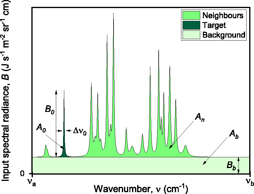
Representation of typical spectral components and their radiance distribution observed typically in Raman measurements. The three main constituents of the spectrum considered here and their key parameters are indicated.

The total radiance entering each spectrometer can therefore be expressed as $A=A_0+A_n+A_b$ .

In accordance with the notation presented in Fig. 1, the contributions to the total radiance from the neighbouring lines and the background continuum can be expressed as a function of the peak value of target line (B₀) by introducing the following parameters

$${\kappa }_n=\frac{A_n}{A_0},{\kappa }_n\ge 0$$

(1a)

$${\kappa }_b=\frac{B_b}{B_0},{\kappa }_b\ge 0$$

(1b)

$${\kappa }_w=\frac{\Delta {\nu }_0}{{\nu }_b-{\nu }_a},0<{\kappa }_w\le 1$$

(1c)

These parameters describe in mathematical terms the richness of the spectral information (κ_n), the background contribution relative to the peak-value of the target line (κ_b) and spectral sharpness of the target line relative to the total bandwidth of the spectrometer (κ_w). It follows that, by using the definition of $\Delta {\nu }_0$ , we can introduce the following relationships

$$A_0=B_0\Delta {\nu }_0=B_0{\kappa }_w({\nu }_b-{\nu }_a)$$

(2a)

$$A_b=B_b({\nu }_b-{\nu }_a)$$

(2b) from which we obtain the following expression for the total radiance

$$A=B_0[{\kappa }_w(1+{\kappa }_n)+{\kappa }_b]({\nu }_b-{\nu }_a)$$

(3)

Equations 1 to 3 will be used in the next sections to provide for each spectrometer a set of generalised equations for the noise and SNR estimates. Limit cases of these equations will be presented for a subset of spectral regimes which are of practical importance in real-life applications of Raman spectroscopy (e.g., a complex multi-component spectrum with minimal background level, and a narrowband spectrum of isolated line with large background contribution) and are related to the limit values of the parameters in Eq. 1.

Grating Spectrometer

A grating spectrometer uses a diffraction grating to spatially disperse the spectral components of the input light along the detector array. The instrument design and optical properties of the diffraction grating determine the spectral resolution and spectral range mapped over the detector array. The spectrum of the input light is reconstructed by recording signal intensities in the spatial domain and by directly mapping the detector pixels to the optical wavelengths.

Figure 2 illustrates a simulated spectrum returned by a grating spectrometer when collecting Raman light with the same spectral components and radiance as those shown in Fig. 1.

Figure 2.

Simulation of the spectrum, S, returned by the grating spectrometer. The values of the key parameters in the model are: N = 1024; 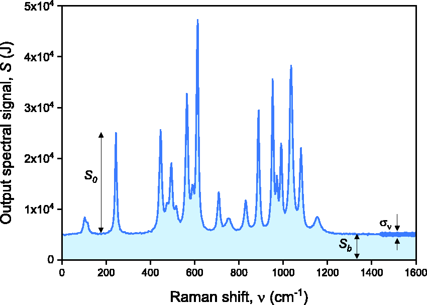$\Delta x=20$ μm; $\Delta =3$ cm^{– 1} ; $S_0=2\times {10}^4$ J; ${\kappa }_b=0.25$ ; G = 1 sr m²; $\Delta t=1$ s.

The magnitude of each data point in the reconstructed spectrum is given by S $(\nu )$  =  $L(\nu )$ G $\Delta t$ , measured in [J] (i.e., the number of photons scaled by the wavenumber-dependent photon energy). The $L(\nu )$ term describes the radiance incident on each detector pixel, G is the spectrometer’s throughput and $\Delta t$ is the total measurement time.

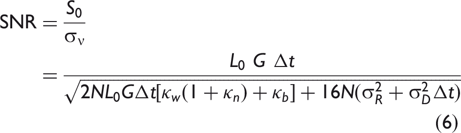
The linear transformation between the signals in the spatial and spectral domains leads to a noise level in the reconstructed spectrum that is governed solely by the statistics of the underlying background signal continuum. In accordance with the notation in Fig. 2 and Eq. 1, this results in the following expression for the SNR of a GS

$\begin{array}{c}\text{SNR}=\frac{S_0}{{\sigma }_{\nu }}\\ =\frac{S_0}{\sqrt{S_b+{\sigma }_R^2+{\sigma }_D^2\Delta t}}\\ =\frac{L_{0}G\Delta t}{\sqrt{{\kappa }_b{L}_0\hspace{1em}G\Delta t+{\sigma }_R^2+{\sigma }_D^2\Delta t}}\end{array}$

(4) where the S₀ is the peak value of the target line in the reconstructed spectrum, and the ${\sigma }_S^2=S_b={\kappa }_b{S}_0$ term originates from the shot noise contribution being proportional to the square root of the background signal.

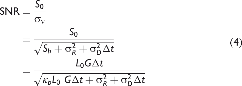
Equation 4 highlights the well-known facts that the SNR of a grating spectrometer does not depend on the spectral richness of the input light. Under detection regimes where the shot noise component of the measured signal dominates over the readout and dark current contributions, Eq. 4 is reduced to

$$\text{SNR}=\sqrt{\frac{L_{0}G\Delta t}{{\kappa }_b}}$$

(5) which highlights that the noise in the reconstructed spectrum is inversely proportional to the square root of the background signal level.

Spatial Heterodyne Spectrometer

The spatial heterodyne spectrometer considered in this work is based on the most established SHS design, which is a modified Michelson arrangement where the two return mirrors are replaced with fixed diffraction gratings.^2,3 For each wavenumber in the wavefront entering the spectrometer, the chromatic dispersion brought by the gratings introduces a wavenumber-dependent crossing angle between the two planar wavefronts interfering at the plane of a detector array. A zero crossing angle is observed for a specific wavenumber, which determines the position of the spectral bandwidth within the electromagnetic spectrum.

The interference pattern resulting from the superimposition of Fizeau fringes with wavenumber-dependent spatial frequencies is recorded simultaneously by all the pixels in the detector array. The spatially modulated signal, Y(x), recorded along the detector array (spatial domain) is subsequently Fourier transformed to reconstruct the spectrum, $S(\nu )$ , of the input light (spectral domain). This is fundamentally different from the case of GS, where the transformation between the spatial and spectral domains is linear.

Examples of the detector signal, Y(x), and output spectrum, $S(\nu )$ , returned by a SHS are shown in Figs. 3a and 3b, respectively, for which the spectral components and input radiance are the same as those chosen for simulating the output spectrum of a GS (Fig. 2). It is important to note that the simulations in Figs. 2 and 3 assume that the two spectrometers have the same measurement times and etendue value.

Figure 3.

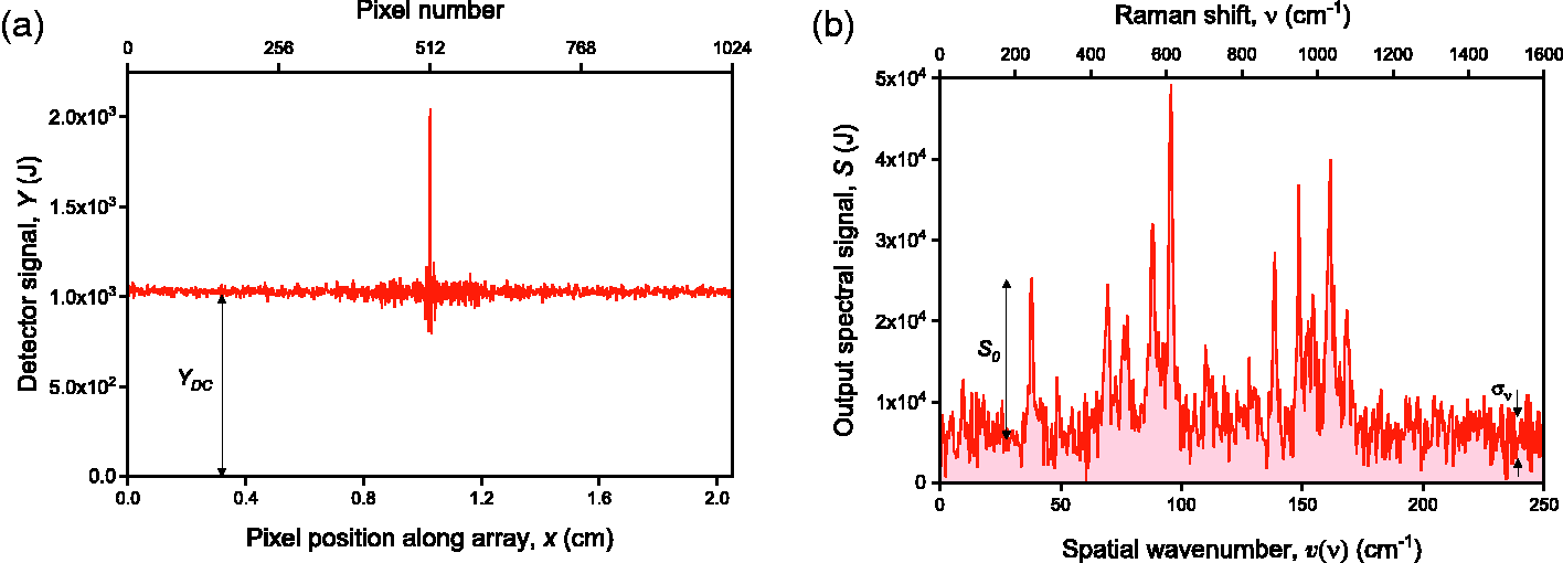
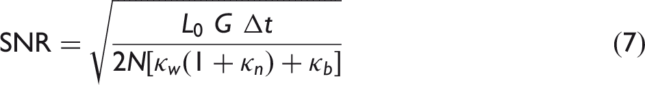
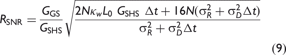
Simulations of (a) the detector signal, Y, and (b) the spectrum, S, returned by the spatial heterodyne spectrometer. The scaling between the spatial wavenumber (v) and spectral wavenumbers ( $=k_{H}v$ ) depends on the spatial heterodyne scheme and specifications of the heterodyning optics. The values of key parameters in the model are: N = 1024; $\Delta x=20$ μm; $k_H=6.413$ ; $\Delta v=0.49$ cm^–1 ( $\Delta =3$ cm^–1); $S_0=2\times {10}^4$ J; $\Delta {\hspace{0.17em}}_{s0}=1.4$ cm^–1 ( $\Delta {\hspace{0.17em}}_0=9$ cm^–1); $A=2.1\times {10}^6$ J s^–1 m^–2sr^–1 (integrated in the $v()$ domain); ${\kappa }_n=18.5$ ; ${\kappa }_b=0.25$ ; ${\kappa }_w=0.0056$ ; G = 1 sr m²; $\Delta t=1$ s. The simulation assumes that the SHS has the same etendue value of the GS simulated in Fig. 2 ( $G_{\text{SHS}}=G_{\text{GS}}$ ).

In terms of the noise analysis, the FT nature of the SHS means that the noise level in the reconstructed spectrum can be estimated by Fourier transforming the noise component of the signal measured by the detector array. A detailed examination of the mathematical workframe can be found in the Supplemental Material. By separating the contributions from each of the three spectral components of the input spectrum according to Eqs. 1 to 3, the noise analysis leads to the following estimate for the SNR of a SHS

$\begin{array}{c}\text{SNR}=\frac{S_0}{{\sigma }_{\nu }}\\ =\frac{L_0\hspace{1em}G\hspace{1em}\Delta t}{\sqrt{2{\mathit{NL}}_{0}G\Delta t[{\kappa }_w(1+{\kappa }_n)+{\kappa }_b]+16N({\sigma }_R^2+{\sigma }_D^2\Delta t)}}\end{array}$

(6)

As for the case of a GS, the L₀ term describes the radiance incident on the detector pixel corresponding to the wavelength of the Raman line, G is the SHS’s throughput and $\Delta t$ is the total measurement time.

Under detection regimes where the shot noise component of the measured signal dominates over the readout and dark current contributions, Eq. 6 can be reduced to

$\text{SNR}=\sqrt{\frac{L_0\hspace{1em}G\hspace{1em}\Delta t}{2N[{\kappa }_w(1+{\kappa }_n)+{\kappa }_b]}}$

(7)

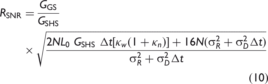
The key practical consequences captured by Eq. 5 are that, for a given peak value of the target Raman line, the SNR of a SHS system is deteriorated by the increase of each of the following parameters: (i) the number of pixels in the detector array (N); (ii) the spectral width of the target line relative to the measured spectral range (κ_w); (iii) the spectral richness of the input light (κ_n); (iv) the magnitude of the background level relative to that of the Raman line (κ_b). Conversely, only the last parameter affects the SNR of a GS system.

Comparison of SNRs

Under the assumption that both spectrometers have the same measurement time, we obtain from Eq. 4 and Eq. 6 that the ratio of the SNR values of a GS over that of a SHS is given by

$\begin{array}{c}{R}_{\text{SNR}}=\frac{{\text{SNR}}_{\mathit{GS}}}{{\text{SNR}}_{\mathit{SHS}}}=\frac{G_{\text{GS}}}{G_{\text{SHS}}}\\ \times \sqrt{\frac{2{\mathit{NL}}_0{G}_{\text{SHS}}\Delta t[{\kappa }_w(1+{\kappa }_n)+{\kappa }_b]+16N({\sigma }_R^2+{\sigma }_D^2\Delta t)}{{\kappa }_b{L}_0\hspace{1em}{G}_{\text{GS}}\hspace{1em}\Delta t+{\sigma }_R^2+{\sigma }_D^2\Delta t}}\end{array}$

(8)

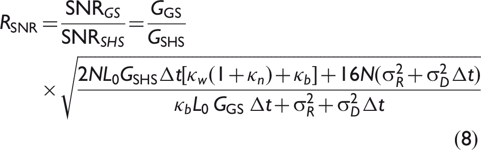
This equation allows to readily map the relative performance of the two spectrometers onto the instrumental and spectral parameters’ space. The simulated trends in Fig. 4 capture some of the key information encapsulated in Eq. 8 by plotting the values of the SNR for each spectrometer and their ratio against two of the parameters describing the spectral properties of the input light: κ_n (spectral richness) and κ_b (background level).

Figure 4.

Signal-to-noise ratio (SNR) estimates for the GS and SHS, and their ratio, as function of parameters describing the (a) spectral richness, κ_n, and (b) the background level relative to the Raman line, κ_b. The values of the spectral and design parameters used in the simulation are: 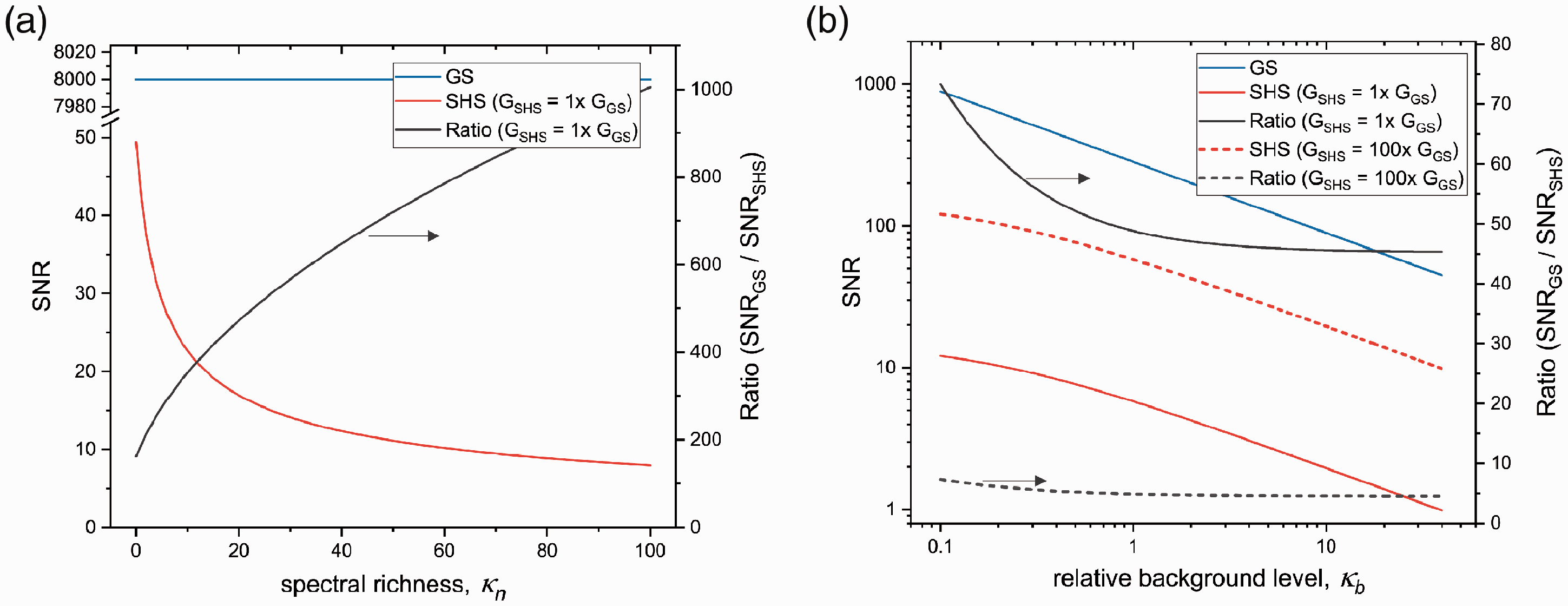$L_0=6\times {10}^4$ J s^–1 m^–2cm; $\Delta \nu =3$ cm^–1; ${\kappa }_w=6\times {10}^{-3}$ ; ${\kappa }_n=25$ ; N = 1024; G = 1 sr m²; $\Delta t=1$ s. The plots in (a) are calculated for ${\kappa }_b=0$ and $G_{\text{SHS}}=G_{\text{GS}}$ . The plots in (b) assume ${\kappa }_n=25$ and are shown for both $G_{\text{SHS}}=G_{\text{GS}}$ and $G_{\text{SHS}}=100\times G_{\text{GS}}$ .

Figure 4a shows that, under the experimental regime where no background signal is present ( ${\kappa }_b=0$ ), the GS outperforms the SHS since only the SNR of the latter is impacted by the presence of dense spectral information.

In real-life Raman measurements, however, some background contribution to the total signal is always present, typically in the form of fluorescence signal. Figure 4b shows that, as the magnitude of this contribution relative to the Raman signal increases, the shot noise component quickly governs the noise levels in both spectrometers. Conversely to the trends in Fig. 4a, the two SNR curves appear offset and decreasing at a very similar rate. The magnitude of the offset depends on the values of the etendue of one spectrometer relative to the other; here, two cases are considered, $G_{\text{SHS}}=G_{\text{GS}}$ (full lines) and $G_{\text{SHS}}=100\times G_{\text{GS}}$ (dashed lines). It is important to note that, for ${\kappa }_b>1$ (background level larger than the Raman signal), the ratio of the two SNR values appears to approach a constant value and becomes independent from the spectral characteristics of the input light. It is worth reiterating that Eq. 8 assumes that the optical components in both spectrometers are assumed to be ideal and lossless; design-dependent losses should be considered in the model to provide a more accurate estimate of $R_{\text{SNR}}$ .

The significance of these results can be emphasised by deriving Eq. 8 for four specific cases of Raman spectra, which are illustrated in Fig. 5.

Figure 5.

Examples of four spectral cases of Raman spectra of practical interest. (a) Case I: Single Raman line, no background; (b) Case II: Complex Raman spectrum, no background; (c) Case III: Complex Raman spectrum with background; (d) Case IV: Bandpass-filtered Raman spectrum with background.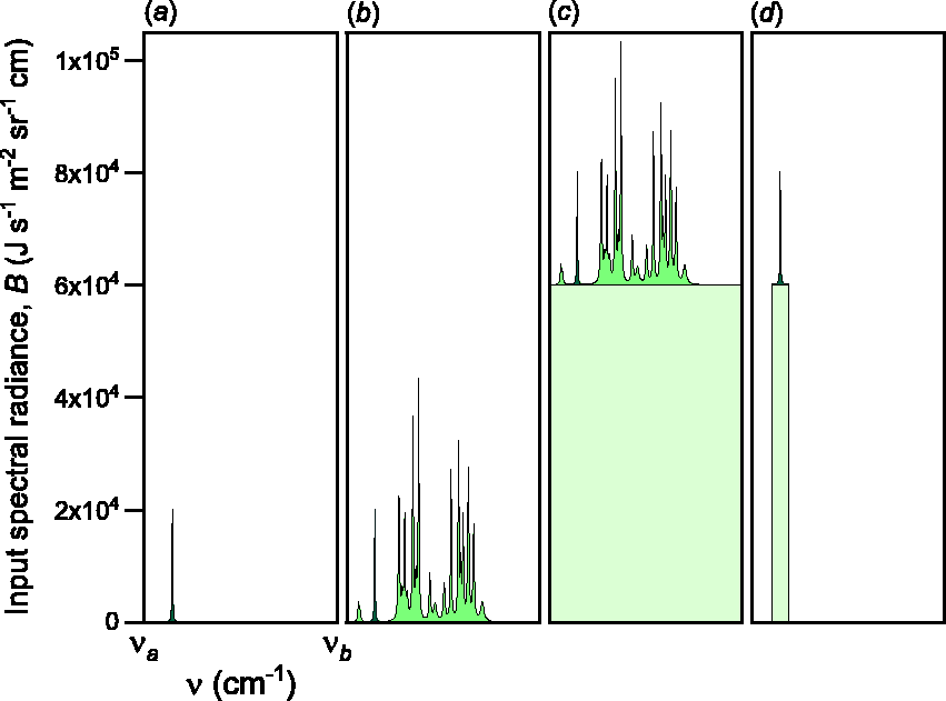

Case I: Single Raman Line, No Background

Under these conditions ( ${\kappa }_n=0,{\kappa }_b=0$ ), Eq. 8 takes the form

$R_{\text{SNR}}=\frac{G_{\text{GS}}}{G_{\text{SHS}}}\sqrt{\frac{2N{\kappa }_w{L}_0\hspace{1em}{G}_{\text{SHS}}\hspace{1em}\Delta t+16N({\sigma }_R^2+{\sigma }_D^2\Delta t)}{{\sigma }_R^2+{\sigma }_D^2\Delta t}}$

(9)

This scenario is rarely encountered in real-life measurements, but it helps appreciating the effects of the spectral properties on the instrument performance.

Case II: Complex Raman Spectrum, No Background

In this spectral regime ( ${\kappa }_n>0,{\kappa }_b=0$ ), Eq. 8 takes the form

$\begin{array}{c}{R}_{\text{SNR}}=\frac{G_{\text{GS}}}{G_{\text{SHS}}}\\ \times \sqrt{\frac{2{\mathit{NL}}_0\hspace{1em}{G}_{\text{SHS}}\hspace{1em}\Delta t[{\kappa }_w(1+{\kappa }_n)]+16N({\sigma }_R^2+{\sigma }_D^2\Delta t)}{{\sigma }_R^2+{\sigma }_D^2\Delta t}}\end{array}$

(10)

This equation emphasises how the spectral richness penalises the performance of the SHS relative to the GS. For the spectrum illustrated in Fig. 5b, the value of $R_{\text{SNR}}$ is 522 (assuming $G_{\text{SHS}}=G_{\text{GS}}$ ).

Case III: Complex Raman Spectrum with Background

In this spectral regime ( ${\kappa }_n>0,{\kappa }_b>>{\kappa }_w(1+{\kappa }_n)$ ), the noise in the recorded signal is most likely dominated by the shot noise contribution, therefore Eq. 8 can be reduced to

$$R_{\text{SNR}}=\sqrt{\frac{G_{\text{GS}}}{G_{\text{SHS}}}}\sqrt{2N}$$

(11)

This is applicable to the majority of Raman spectra commonly observed in most real-life measurements. For the case of the spectrum simulated in Fig. 5c, the ratio between the SNRs values is 45 for $G_{\text{SHS}}=G_{\text{GS}}$ , and drops to $\hspace{1em}\sim 5$ if it assumed that $G_{\text{SHS}}=100\times G_{\text{GS}}$ .

Case IV: Bandpass-filtered Raman Spectrum with Background

In this scenario, Eq. 11 is modified to account for the reduction in the input radiance due to the use of an optical bandpass filter around the target line. This leads to

$$R_{\text{SNR}}=\sqrt{\frac{G_{\text{GS}}}{G_{\text{SHS}}}}\sqrt{2N\alpha }$$

(12) where α represents the ratio of the spectral bandwidth of the bandpass filter relative to the total spectral range accessible by the spectrometer. For the spectrum shown in Fig. 5c, $\alpha =0.08$ , which leads to approximately a three-fold reduction of $R_{\text{SNR}}$ relative to Case III.

Practical Considerations

In real-life applications of Raman spectroscopy, spectrometers are typically operated in shot noise limited regimes of detection and most sample spectra fall under the regime captured by Case III, i.e., a complex Raman spectrum sitting on a broad pedestal associated with fluorescence (and sometimes ambient light). Under these experimental conditions, Eq. 11 indicates that the detection performance of a GS relative to a SHS ( $R_{\text{SNR}}$ ) is governed primarily by two design parameters: the optical throughput achieved by each spectrometer and the number of row pixels in the detector array.

These findings help addressing in quantitative terms the following question: in the context of in-field Raman spectroscopy, which of the two technologies promises the best trade-off between compactness and performance?

The outputs from a preliminary investigation are summarised in Table I. For both types of spectrometers, the values have been selected to meet the requirements of broad spectral coverage (at least the fingerprint region, <1700 cm^–1) and spectral resolution adequate for identification-focused applications (<20 cm^–1). The size of the camera pixel is set to 26 μm (value typical of most commercially available Raman cameras).

Table I.

Comparison between the specifications typical of portable, high-performance Raman spectrometers based on GS and SHS designs.

Parameter	Unit	GS	SHS
Number of row pixels, N		1024	400	800	800
Length of detector array a , L	mm	26.6	10.4	20.8	20.8
Spectral resolution b	cm–1	8	16	8	16
Spectral range	cm–1	1700 (3400)	1700	1700	3400
Solid angle c , Ω	Sr	0.18	0.006	0.003	0.006
Aperture d	mm	0.05 × 6	10.4 × 10.4	20.8 × 20.8	20.8 × 20.8
Aperture area, E	mm 2	0.3	108	432	432
Etendue, $G=E\times \Omega$	mm 2 sr	0.054	0.63	1.26	2.52
$R_{\text{SNR}}$ (Case III) e			8	8	6
Estimated footprint f	cm 3	300	8	27	27

a

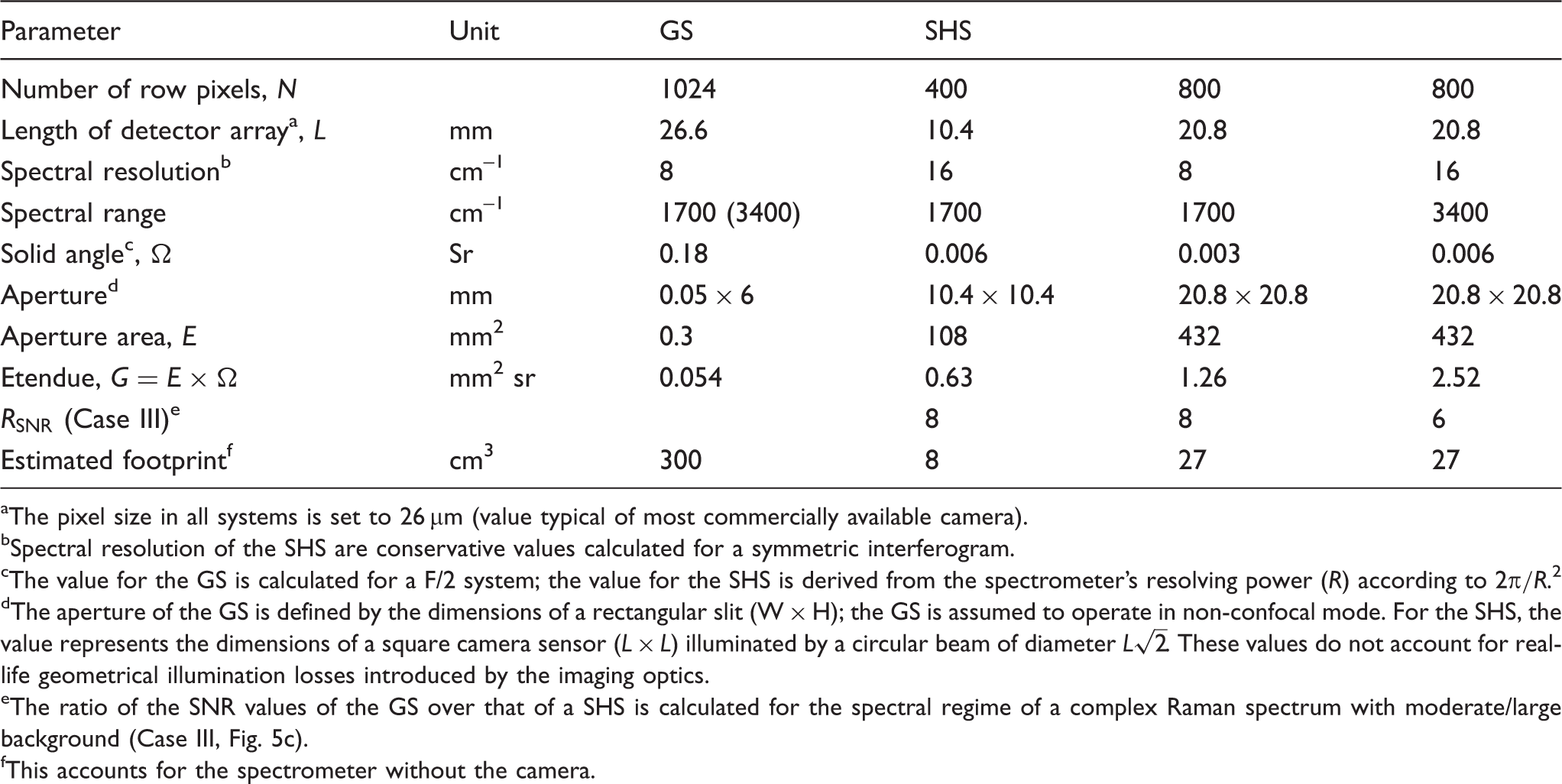
The pixel size in all systems is set to 26 μm (value typical of most commercially available camera).

b

Spectral resolution of the SHS are conservative values calculated for a symmetric interferogram.

c

The value for the GS is calculated for a F/2 system; the value for the SHS is derived from the spectrometer’s resolving power (R) according to $2/R$ . ²

d

The aperture of the GS is defined by the dimensions of a rectangular slit (W × H); the GS is assumed to operate in non-confocal mode. For the SHS, the value represents the dimensions of a square camera sensor (L × L) illuminated by a circular beam of diameter $L\sqrt{2}$ . These values do not account for real-life geometrical illumination losses introduced by the imaging optics.

e

The ratio of the SNR values of the GS over that of a SHS is calculated for the spectral regime of a complex Raman spectrum with moderate/large background (Case III, Fig. 5c).

f

This accounts for the spectrometer without the camera.

The values for the GS are those typically seen for high-performance, portable Raman spectrometers available on the market. For the case of the SHS designs proposed in the table, the fundamental relationships from the theory of spatial heterodyne spectroscopy have been used by the authors to calculate the values of the input parameters that would meet the requirements mentioned above;^2,7 in addition, they assume a square camera format.

From Table I, the following points are worth noting. The entrance aperture of a SHS can be more than two orders of magnitude larger than that of a GS. Conversely, GS instruments typically achieve larger collection angles (although at the cost of a larger footprint).

In the case of a SHS, decreasing the number of row pixels results (for a given pixel size and spectral coverage) in a poorer resolution but in a potentially higher SNR level; this is encapsulated in Eq. 11, and is due to a larger achievable solid angle (according to $\Omega =2/R$ , where R is the resolving power ² ) together with the lower spatial dilution of the input radiance (i.e., each pixel accepts more photons). Alternatively, a larger spectral coverage can be traded for a poorer resolution (for a given size and number of pixels), which can lead to a larger solid angle and therefore to an increase of the SNR.

For the sets of input values presented in Table I, we can conclude that SHS systems lend themselves to a level of miniaturisation much greater than typical portable, high-performance GS designs, but their SNR levels are expected to be about five to ten times lower.

It is important to note, however, that this estimate is only indicative. On one hand, optical aberrations and background signal contributions from ambient or out-of-band light can rapidly deteriorate the performance of SHS by reducing the fringe visibility. On the other hand, established SHS design strategies, such as the use of field-widening prisms ¹⁵ or asymmetric interferogram sampling, ¹ have the potential to help reducing further the performance gap between the two technologies.

Conclusion

In this work, the detection performance of Raman spectrometers based on GS and SHS designs have been estimated and compared in quantitative terms by deriving the analytical expressions for the performance estimator (SNR) for both types of spectrometers.

The analysis shows that, depending on the spectral characteristics of the Raman light and on the values of some instrument-specific parameters, the ratio of the SNR estimates for the two types of spectrometer ( $R_{\text{SNR}}$ , as defined in Eq. 8) can vary as much as by two orders of magnitude. In particular, under the experimental conditions where the background signal is comparable or larger than the target Raman line and shot noise is the dominant noise contribution, the value of $R_{\text{SNR}}$ is, to a first order of approximation, dependent solely on the relative values of each spectrometer’s etendue and on the number of pixels in the detector array (Eq. 11). It is worth pointing out that these estimates do not account for the real efficiencies of the optical components and camera illumination, and therefore this model should be customised to the specific GS and SHS designs under consideration.

The practical consequences of these conclusions are captured in Table I, which reports the values of the key instrumental parameters expected for typical portable GS and SHS systems, and their impact on the value of $R_{\text{SNR}}$ under the experimental conditions described above (Fig. 5c). For the specific designs considered in the table, we can conclude that, despite the fundamental noise penalty typical of FT spectrometer operating in shot noise regimes of detection, SHS-based Raman spectrometers have the potential to compete with compact GS designs for delivering in a much smaller footprint (10–30 times) ⁶ levels of detection performance that are only five to ten times poorer.

In more general terms, it is the authors’ view that, in the context of Raman measurements, SHS designs will very unlikely exceed the levels of detection sensitivities of GS with comparable spectral resolution and range. However, for applications where miniaturisation is a key requirement and could be traded for a small reduction in spectral and detection performance, the SHS could become the go-to solution in the future landscape of portable Raman spectroscopy.

Supplemental Material

sj-pdf-1-asp-10.1177_0003702820957311 - Supplemental material for Grating Spectrometry and Spatial Heterodyne Fourier Transform Spectrometry: Comparative Noise Analysis for Raman Measurements

Supplemental material, sj-pdf-1-asp-10.1177_0003702820957311 for Grating Spectrometry and Spatial Heterodyne Fourier Transform Spectrometry: Comparative Noise Analysis for Raman Measurements by Luca Ciaffoni, Pavel Matousek, William Parker, Elin A. McCormack and Hugh Mortimer in Applied Spectroscopy