Sage Journals: Discover world-class research

Abstract

Rising inequalities in rich countries have led to concerns that the economic ladder is getting harder to climb. Yet, research on trends in intergenerational income mobility finds conflicting results. To better understand this variation, we adopt a multiverse approach that estimates trends over 82,944 different definitions of income mobility, varying how and for whom income is measured. Our analysis draws on comprehensive register data for Swedish cohorts born 1958 to 1977 and their parents. We find that income mobility has declined, but for reasons neglected by previous research: improved gender equality in the labor market raises intergenerational persistence in women’s earnings and the household incomes of both men and women. Dominant theories that focus on childhood investments have blinded researchers to this development. Methodologically, we show how multiverse analysis can be used with abduction—inference to the best explanation—to improve theory-building in social science.

Keywords

intergenerational mobility multiverse analysis open science transparency abductive inference

The late-twentieth century saw earnings and wealth inequality rise in most Western countries. This has sparked concerns about the consequences for younger generations. Do increased disparities mean a child’s family of upbringing has become more important as a predictor of their attainment as an adult? Research to date provides no conclusive answer: studies in the United States and in Scandinavia—the context of this study—report everything from no trend to a decrease in income mobility, or even a slight increase (Aaronson and Mazumder 2008; Bloome 2015; Bloome, Dyer, and Zhou 2018; Bratberg, Nilsen, and Vaage 2007; Chetty et al. 2014b; Davis and Mazumder 2020; Fertig 2003; Hansen 2010; Hansen and Toft 2021; Harding and Munk 2020; Hertz 2007; Jonsson, Mood, and Bihagen 2011; Lee and Solon 2009; Mayer and Lopoo 2005; Pekkala and Lucas 2007; Pekkarinen, Salvanes, and Sarvimäki 2017; Sirniö, Kauppinen, and Martikainen 2017).

How has a question so important eluded a clear answer? Some indeterminacy may be due to arbitrary differences in, for example, sample or time span. If so, as more and better data become available, studies will eventually converge. Alternatively, these studies might have been asking not one but several questions, through subtle differences in target parameter or study design. The literature on intergenerational income mobility works with a wide range of models and definitions. While the question “Has mobility decreased?” is generic, different models can speak to different estimands (Lundberg, Johnson, and Stewart 2021). If so, variation is an irreducible feature, and no matter how much data we have, studies may not converge on a single answer.

As we will argue, the way forward lies in treating model variation not as a nuisance but as an indispensable source of information. In this study we focus on Sweden, where access to five decades of population data allows us to estimate a wide range of models. We ask how levels of and trends in intergenerational income mobility depend on the choice of income concept, differences between men and women, the age and period at which income is measured, how zero values are treated, and the parameter of association. Our use of a single high-quality dataset lets us abstract from variation due to context, sampling, or measurement error. We examine 20 cohorts and 82,944 alternative specifications.

Our work extends current efforts to increase transparency in social science (Freese, Rauf, and Voelkel 2022). Specifically, we use “multiverse analysis,” a procedure that exhausts all possible combinations that arise from a set of reasonable analytic choices (Berk, Brown, and Zhao 2010; Muñoz and Young 2018; Western 1996). Tools for increased transparency have yet to gain widespread adoption. One reason, we believe, is that the solutions they offer are often wedded to a deductive paradigm quite far removed from what many social scientists actually do. Existing uses of multiverse analysis treat model uncertainty as akin to sampling variance, indicating the “robustness” of results. On this view, model variance is a bad thing: the more results vary across specifications, the weaker the support for a given hypothesis. This risks imposing unreasonable standards, because variation is almost always rife.

In this article, we argue that increased transparency can help foster a different model of inquiry that, incidentally, better represents what many sociologists have always done. Instead of testing a given hypothesis derived from theory, we ask: what explanation best accounts for the sum of results? This approach, known as abduction or inference to the best explanation (Lipton 2003; Peirce 1974), provides a powerful model for how transparency can accelerate knowledge production. In this alternative model, the goal is not to accept or refute a given hypothesis, but rather to generate a wide range of observations that help modify and improve upon existing theory (Brandt and Timmermans 2021; Lieberson and Horwich 2008). We address quantitative researchers, but parallel arguments have been put forth in the qualitative literature (Tavory and Timmermans 2014).

Substantively, we find that mobility has declined in recent cohorts, but for reasons neglected by previous literature. The most consistent contributor to trends is the advancement of women in the labor market, which leads to increased persistence in women’s earnings. Importantly, this influence shows not only in women’s own incomes but also in the household incomes of both men and women. For specifications that isolate men’s earnings, mobility has mostly remained flat or increased. In other words, intergenerational mobility is declining as women are realizing their earnings potential to a greater degree.

We also contribute to several methodological strands of the income mobility literature. Recent research has abandoned measures based on log income in favor of rank-based approaches that are supposedly more robust (Bloome et al. 2018; Chetty et al. 2014a; Dahl and DeLeire 2008). At the same time, it is often presumed that log-based measures are preferable when data limitations do not preclude their use (Mazumder 2016; Mitnik, Bryant, and Weber 2019; Mitnik and Grusky 2020). We move this debate forward by showing that (1) rank-based measures are far from insensitive to considerations such as life-cycle bias, and (2) log-based measures behave erratically even with close to ideal data, due to an extreme dependence on the bottom of the distribution.

Ultimately, our study offers an opportunity for scholars to put past and future work on income mobility in context, and gauge how it may reflect the combinations of decisions reached by authors.¹ Because studies often differ in more than one dimension, it is hard to draw out the implications of differences across them. Yet, for research in the field to be cumulative, we must know the consequences of different income definitions and model specifications. A multiverse analysis formalizes this process and provides a yardstick by which to contextualize studies that only explore a small part of the model space. Moreover, such knowledge can move the field from broad descriptions toward a deeper understanding of the mechanisms behind intergenerational persistence.

Previous Research On Income Mobility

The extent to which poverty or riches are perpetuated across generations has long been a topic of social concern. A high degree of intergenerational mobility is generally viewed as desirable, being a proxy for a society that offers equal opportunities (Breen and Jonsson 2005). Mobility is typically measured by the strength of the association in status between generations. In the case of income, this becomes a correlation or regression coefficient from an equation where parent income is used to predict the income of the child. In other words, the basic datum of mobility research is a measure of its inverse: intergenerational transmission or persistence.

Country Differences

The maturation of income mobility as a field is largely a story of how researchers learned to address two sources of variation: measurement error and life-cycle bias. In one of the earliest reviews, Becker and Tomes (1986:S32) concluded that “regression to the mean . . . appears to be rapid” and relative earnings differences between families are mostly “wiped out in three generations.”

Today, we know this conclusion was premature and stemmed from studies using snapshots of fathers’ and sons’ income that are weak proxies of lifetime income. Solon (1992) was early to point this out, and over the following decades, a string of studies led to a gradual revision upward of the estimated association. Current best estimates suggest that at least as much as half of earnings inequality is inherited in the United States today (Cheng and Song 2019; Gregg, Jonsson, et al. 2017; Mazumder 2016; Mitnik et al. 2019).

Along with the accumulation of U.S. evidence, estimates also surfaced for other countries. Björklund and Jäntti (1997) showed that persistence of incomes was less pronounced in Sweden, a Scandinavian-type welfare state. Their results contradicted the notion of the United States as a “land of opportunity,” where high inequality in the cross-section is offset by the absence of a rigid class structure. The idea that more equal countries provide a more level playing field soon gained traction and was eventually epitomized in the “Great Gatsby Curve” (henceforth GGC; Corak 2013), a graph showing that high income inequality tends to go together with less income mobility.

Time Trends

Most wealthy countries have seen income inequality grow since the 1970s or 1980s. If we believe the GGC reflects a causal relationship, we would expect intergenerational transmission to rise with inequality over time. Here the evidence is much less consistent (Torche 2015). The best available data for the United States suggest no trend in income mobility for cohorts born from the 1970s through the 1980s (Chetty et al. 2014b). Earlier U.S. studies reached similar conclusions, including Hertz (2007), Lee and Solon (2009), and Bloome (2015). However, this has been contradicted by studies claiming to detect a mobility decline (Aaronson and Mazumder 2008; Davis and Mazumder 2020), or even an increase in mobility (Fertig 2003; Mayer and Lopoo 2005).

There is some evidence for Scandinavia: Bratberg and colleagues (2007), Hansen (2010), and Pekkarinen and colleagues (2017) in Norway, and Pekkala and Lucas (2007) in Finland, all find a tendency toward equalization in cohorts born before 1960 and stable or slightly increasing persistence thereafter, but the results are sometimes sensitive to alternative specifications. Jonsson and colleagues (2011) find an increasing elasticity but a decreasing correlation over Swedish cohorts born 1960 to 1970. Harding and Munk (2020) study the intergenerational rank correlation in family income with Danish data, and report that income persistence increased among both men and women from cohorts born in the late 1950s onward.

Related evidence comes from sibling correlations. Here, Björklund, Jäntti, and Lindquist (2009) find decreasing income correlations for Swedish brothers born until 1950 and a slight increase thereafter. Wiborg and Hansen (2018) report a similar increase in earnings and wealth correlations among recent cohorts of Norwegian brothers and sisters. Also in Norway, Hansen and Toft (2021) find that class-origin income gaps increased for daughters but remained stable for sons, whereas class-origin wealth gaps increased for both sexes.

Abductive Multiverse Analysis

That previous studies have reached mixed results is not surprising. Studies cover different contexts and populations, but also vary in other respects. Any statistical analysis faces a wide range of options in how to set up or clean the data, construct key variables, treat missing or extreme values, select functional form, the estimation method, and so on. Some alternatives may be unavailable and beyond the researcher’s control; others are subject to choices that must be made more or less consciously. Without a systematic approach to heterogeneity, it is difficult to learn from these varied results. A multiverse analysis renders the variation transparent by considering the consequences of every alternative choice.

Existing uses of multiverse analysis presuppose that a researcher aims to test one hypothesis, and they treat variation as indicating the “robustness” of results (Muñoz and Young 2018; Simonsohn, Simmons, and Nelson 2020; Steegen et al. 2016; Young and Holsteen 2017). The more specifications a given result survives, supposedly the stronger the evidence. On this approach, a researcher would use theory or a hunch to develop a prediction of the form: “mobility is declining.” Testing the prediction under a range of specifications may then render it disconfirmed, robustly confirmed across multiple specifications, or “remarkably dependent on a knife-edge specification” (Young 2018).

In our view, this multiverse-as-robustness approach fails to fully capitalize on the data. Different specifications can speak to different questions in ways that are not obvious before a researcher sets out on an analysis. If we find that mobility appears to be declining under some specifications but not others, the logical next step is to ask what characterizes these specifications. This is the essence of the approach we propose here, abductive multiverse analysis. Unlike deduction, abduction is not intended to test hypotheses, but to come up with them (Brandt and Timmermans 2021). Unlike induction, it goes beyond simple generalization to engage theory, in ways we elaborate next.

The Role of Theory

Under a deductive model, the aim of theory is to provide predictions that can be tested against data. Call this the “map” view of theorizing. The theory provides the roadmap to an outcome; if at the end of the road we find the predicted outcome, we consider the theory at least provisionally valid. This deductive model is what we aspire to when we structure our writing around hypotheses, significance tests, and so on—although it is an open secret that these trappings of scientific rigor often enter at a late stage of the process.

In the world that sociologists inhabit, a more flexible interplay between theory and data would seem more fitting to many research problems. With abduction, or inference to the best explanation (Lipton 2003; Merton 1987; Peirce 1974), theory is not used to derive sharp predictions. Rather, it serves as a scaffold to arrange a set of loosely held beliefs that may be revised as evidence continues to build. Call this the “scaffolding” view of theorizing. Here, theories meet the data not in a binary confirmation-or-refutation way, but by using heterogeneous results to get at scope conditions and eventually, underlying mechanisms.²

This model of knowledge accumulation has been likened to the way a crossword puzzle is solved, by carefully fitting pieces of evidence until only one plausible explanation remains (Haack 2000), an approach found in many classical works. We can see it in Weber’s analysis of the economic effects of Protestantism, in Durkheim’s analysis of suicide, and in Darwin’s development of the theory of natural selection. John Snow’s pioneering work on cholera in the 1850s, often cited as a forerunner in causal inference, has more in common with the crossword model than with modern causal inference (Freedman 1991).

Assumptions of Previous Research

Entering a field with too strong priors risks blinding us to plausible alternatives. Take the “Great Gatsby” argument. What ostensibly is a simple prediction—mobility will decrease with rising inequality—encompasses a host of assumptions about how and why. Focusing on parental investments, it assumes intergenerational association represents, at least partly, a causal effect of income (Mayer 1997). By centering the role of inequality during childhood, it reinforces the “economization of early life” (Griffen 2023). This focus on the family, in turn, risks detracting from wider societal factors, such as market imperfections or power struggles in the arena of work.

Recent neglect of the labor market in intergenerational mobility has a parallel in the status attainment paradigm, once dominant in stratification research (Sewell, Haller, and Portes 1969; Sewell and Hauser 1975). Like the Becker and Tomes (1979, 1986) framework that guides income mobility research today, status attainment emphasized processes linking individual orientations to education and subsequent jobs. Yet, it remained silent on structural sources of inequality in the labor market, and the fraught social and political choices that link jobs to rewards (Baron and Bielby 1980; Engzell and Wilmers 2023; Tomaskovic-Devey and Avent-Holt 2019).

Dominant paradigms tend to be durable and self-reinforcing. The types of questions asked depend on available data, and the questions asked then shape how data are collected, curated, and analyzed (Hirschman 2021). If we see intergenerational persistence rising with inequality, it is easy to take this as confirmation of a causal chain from parental investments to mobility. In reality, mobility might shift for many reasons, only some of them driven by parenting. A more flexible interplay between theory and data can lead us out of such ignorance traps and point toward better and revised theories (Lieberson and Horwich 2008).

A Model Of Intergenerational Mobility

We sketch a model of intergenerational income mobility in Figure 1. This model, which we borrow from Breen and Jonsson (2007), incorporates key components of the status attainment and Becker–Tomes models.³ It is deliberately flexible: its purpose is not to serve as a map yielding sharp predictions, but as a scaffold to help make sense of heterogeneous results.

Figure 1.

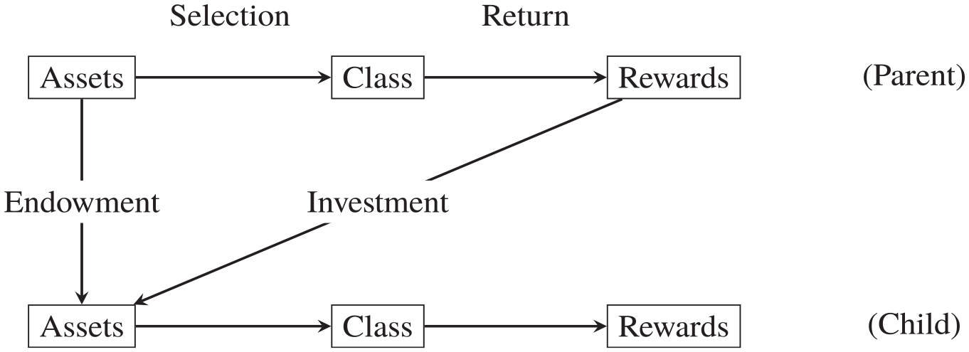
A Model of Intergenerational Mobility

Mobility can be seen as a series of interlinked processes (cf. Breen and Jonsson 2007; Grusky and Szelenyi 2018): First, a system of socialization that endows children with unequal amounts of cultural and social capital (“assets”). Such traits are often constitutive of the individual, inalienable, and embedded in one’s identity. Second, a system of institutional differentiation that enables personal traits to be converted into recognized, institutional markers of status, such as educational qualifications or job titles (“class”). And third, a system of reward that endows different locations in the class structure with unequal compensation (“rewards”).

Income mobility captures the correlation of rewards across generations. It follows that a change in mobility can come about through a change in any one of the six paths in Figure 1.⁴ The common hypothesis that inequality will hamper mobility rests on extrapolating from one trend (inequality) through one pathway (parental investments). A deductive approach to testing it would have to make the heroic assumption that everything else in the system stays constant. The abductive approach we take lets the data speak first, and only then seeks to identify the most plausible explanation for the patterns identified.

The Swedish Context

The increase in inequality across rich countries is well documented, and started around the mid-1970s in the U.S. case (Morris and Western 1999; Neckerman and Torche 2007). In Scandinavian countries, income inequality did not start to rise until the 1980s, and took off significantly after the recession in the 1990s (Jonsson, Mood, and Bihagen 2016). While Sweden is known as a redistributive welfare state with extensive social safety nets, the rise in inequality has been more pronounced in disposable incomes than in labor earnings (Jonsson et al. 2011). This is due to a lowering of real taxes and benefits and a steep rise in capital incomes.

Our cohorts (1958 to 1977) grew up during a time of increasing equality but experienced the labor market during one of increasing inequality. It is hard to know whether the decreasing inequality during childhood or rising inequality later in life should guide the prediction of mobility across these cohorts. The typical argument emphasizes childhood, with inequality magnifying “the difference in the capacities of rich and poor families to invest in their children” (Ermisch et al. 2018:501). At the same time, other authors have emphasized the role of inequality when children enter the labor market (e.g., Davis and Mazumder 2020).

The formative years of these cohorts saw several other social transformations. Tertiary education, which in Sweden is publicly financed, expanded from about 30 percent enrollment in our first cohorts to nearly 50 percent only a decade later (Jonsson and Erikson 2007). Occupational mobility is higher among college graduates (Hout 1988), but there may be offsetting effects for income (Torche 2016; Zhou 2019). In the generation of both parents and children, couples increasingly became dual breadwinners following a 1970 individualized tax reform (Hwang and Broberg 2014), and women’s and men’s careers have become increasingly similar (Härkönen and Bihagen 2011; Härkönen, Manzoni, and Bihagen 2016).

Women’s inroads into the labor market went together with delayed childbearing, a deinstitutionalization of the family, and a weakening of the link between children and marriage (Gähler and Palmtag 2015). Partly in response, high-quality state-subsidized daycare expanded from the 1960s onward (Andersson, Duvander, and Hank 2004). Women’s changing labor market behavior should matter not only because women will contribute a growing share of family income (Beller 2009; Hansen 2010), but also because realized income becomes a better proxy for their earnings capacity (Gonalons-Pons and Schwartz 2017).

Unemployment rates in Sweden have been rather stable around 6 to 7 percent since the end of the 1990s, which stands in dramatic contrast to the low rates of 2 to 3 percent for the period 1950 to 1990. The dividing line between these periods was the mid-1990s recession, when unemployment rose to around 10 percent and the government instituted several structural economic reforms (Forslund 2008; SCB 2021). Hence, while unemployment was uncommon in the parental generation, it is a more tangible risk in the child generation.

Analytic Roadmap

To study how specifications influence mobility estimates, we first specify a set of choices researchers commonly face. Next, we use all possible combinations of those choices to define the model space. We then estimate all specifications and explore how the parameter of interest varies across them.

To start, we address the question of robustness that typical multiverse analyses focus on. This simply asks about the extent of variation, without seeking to understand its sources. For levels, we pay special attention to the upper bound of persistence estimates, given that Sweden is commonly seen as a high-mobility country. The previous literature contains far more estimates for the United States, with preference typically given to larger estimates (Corak 2006). Recent scholarship questions the idea of high Scandinavian mobility and suggests it is isolated to certain measures (Landersø and Heckman 2017). Given that U.S. estimates reflect a wide search across data sources and specifications, it makes sense to conduct a similar search in a Scandinavian setting.

Our results for levels turn out remarkably consistent with the received view that mobility is high in Sweden. For trends, the story is more mixed. Depending on specification, one could conclude that income mobility is increasing, decreasing, or remaining flat. In the next step, we identify the most influential contributors to levels and trends. We formalize this procedure by inspecting the variance explained (R²) in the outcome space by model components individually and in combination. Some of the patterns we detect defy easy summary, but others reveal insights that become apparent only against the relief of the full model space.

The main upshot of our analysis is that declining mobility appears restricted to specifications that include women’s earnings, either directly or as part of family income. A deductive approach using a single specification might have attributed this decline to rising inequality. Instead, our results suggest a different explanation: progress on gender equality. We corroborate this explanation using our own data as well as auxiliary evidence. This step highlights how abductive analysis is driven neither exclusively by theory nor by data, but represents an interplay between the two.

We base most of our analyses on the intergenerational rank correlation, but we also examine a broader range of parameters. We use this opportunity to contribute to existing methodological debate around income mobility. Prior work generally holds that the intergenerational elasticity is the theoretically preferred measure, but the rank correlation is useful when data have a limited observation span. We question both notions by showing that elasticities behave erratically even with close to ideal data, and rank correlations remain sensitive to life-cycle bias. No measure is immune to considerations of specification, but mapping the full range of variation can help researchers make an informed choice.

Data

Our data consist of the full population of men and women born in Sweden from 1958 to 1977; the number of children we observe is around 100,000 in each annual cohort. Data are merged from various administrative registers. The register of the total population gives basic information about, for example, birth year, country of birth, and sex, and demographic event registers contain information about migration and civil status changes. The multigenerational register contains links between (biological and adoptive) parents and children, covering all children in our cohorts where at least one parent has been registered as resident in Sweden at any point since 1947. In our cohorts, virtually all individuals can be linked to the mother, and 98 to 99 percent to the father. Between .2 and 1.5 percent in a given cohort have a link to both a biological and an adoptive parent of the same sex, and in these cases the adoptive parent is given priority.

Information on earnings and incomes comes from the annual income registers 1968 to 2019. The primary source for the income registers is tax records, covering all taxable incomes and taxes, and to these are added any non-taxable benefits. All incomes are expressed in 2019 prices using Statistics Sweden’s official consumer price index. The zero earnings or incomes in our data are “real” zeros rather than missing values insofar as the target quantity is official Swedish income/earnings, but people with zero observed incomes can have undisclosed foreign income or income from unofficial sources. The only missing values on income are for individuals who are not registered as resident in Sweden in a given year (due to either migration or death). We top-code incomes higher than four standard deviations above the mean, which matters only for the linear correlation.⁵

Earnings are defined as the sum of individual pre-tax salary, self-employment income, and (from 1974) taxable earnings-related social insurance benefits (e.g., parenting or sickness payment). Inclusion of social insurance benefits makes only a slight difference to estimates (Mood 2017). Disposable personal income is defined as earnings (as defined above), and all other registered taxable and tax-free income, subtracting taxes. In contrast to earnings, it includes redistributing components but also incomes from capital. The disposable family income is the sum of the personal disposable incomes of the adults in the household (excluding incomes of any adult children living with parents). For parents, this variable is the same in a given year (but not at a given age if parents differ in age) if they live together, but if they are separated this variable captures the income of the new (single-adult or reconstituted) family.

Restriction to the specific cohorts we study is dictated by a number of data demands. The lower bound, 1958, is motivated by the fact that full-population income data are only available from the year 1968 onward. Thus, while we are able to link offspring to their parents further back, we want to record parental incomes at a time when the children grew up (or, at least, when their parents were still active in the labor market). With the current selection, most of the parents in the oldest cohort are between ages 30 and 50 at the time when they first appear in our income data. The upper bound, 1977, is imposed to be able to observe offspring earnings at prime ages of labor market activity (up until age 42).

Sources Of Model Variation

We address five sources of variation: (1) income concept, (2) differences between men and women, (3) the age and period at which income is measured, (4) how to treat zero values, and (5) the parameter of association. These dimensions often vary in the existing literature.

Our use of the term “specification” is deliberately broad. Whether to study women, men, or both is a different kind of choice than how to treat zero incomes, or at which age to observe income. Some alternatives clearly speak to different questions, and others seem more arbitrary from a theoretical standpoint. However, theoretical concerns are seldom explicit when authors present a given specification. Moreover, even choices that seem to carry less theoretical weight may, upon inspection, turn out to have a more substantive interpretation than thought. Therefore, we refrain from distinguishing a priori between dimensions that are more or less theoretically important.

Income Concept

Income has been defined in various ways in the literature. We distinguish between labor earnings, disposable personal income, and disposable family income (see the Data section), and allow any combination of them on the left-hand and right-hand side.

One can easily conceive of different combinations of parent and child income measures as more or less suitable depending on the question motivating the study. If we are interested in how parents’ economic investments translate into unequal attainments, we should study parents’ disposable income during the child’s formative years. By contrast, if we believe that parents transmit (genetically or culturally) traits that enhance a child’s income, labor earnings are the appropriate proxy. Similarly, different outcome measures may be relevant depending on whether we are interested in children’s living standard or their capacity to generate earnings in the labor market.

The common focus on parental investments would suggest using disposable family income, possibly equivalized for household size. Until recently, the standard has instead been to focus on men’s labor earnings. Lately it has become more common to use family income in both the parent and child generations (Bloome et al. 2018; Chetty et al. 2014a). This is a more encompassing measure of living standards, and more aligned with theories emphasizing investment. Family income also makes women and men look more similar and may therefore seem like a tempting way to abstract from sex. At the same time, it brings in mechanisms of partner selection and family formation that can make estimates hard to interpret (Chadwick and Solon 2002; Choi, Chung, and Breen 2020; Holmlund 2022).

Parent and Child Sex

For a long time, it was common to study the intergenerational mobility of men to the exclusion of women. This is an understandable choice if most women do not participate in the labor force, but that time has long passed, making the near-exclusive focus on men untenable (Beller 2009; Charles 2011; Goldin 2006; Hout 2018). Results for women are still not as common as those for men, but they tend to show that women’s labor market attainment is less strongly predicted by parental origin than that of men, leading some to conclude there is greater equality of opportunity among women than among men (Hederos, Jäntti, and Lindahl 2017). We study mothers, daughters, fathers, and sons separately.

Age and Observation Window

What is the appropriate age to observe income? We measure income of parents centered around ages 35, 40, 45, and 50, and for the offspring centered around ages 25, 30, 35, and 40. For each of these ages, we study incomes for single years, or averaged over all non-missing observations over three and five years, respectively. In supplementary analyses, we expand the observation window to more than 30 years for both parents and children.

This dimension is subject to a large literature on its own, centering on the twin issues of transitory income shocks and life-cycle bias (Haider and Solon 2006; Jenkins 1987). The quest to mitigate these sources of bias has guided the literature, giving rise to shifting conventions over the years. There are three reasons why we address these issues, despite extensive coverage in earlier work. First, given the heavy emphasis on these issues in the literature, it is worth knowing how important age and observation window are relative to other, less-recognized sources of variation. Second, we make a new contribution by studying how these and other dimensions interact to produce variation. Third, work on life-cycle bias has mainly focused on mobility levels, and we know less about how it may affect trends.

Theoretical models of income transmission often refer to lifetime income, that is, income accumulated over the whole career (Solon 2004). If this is the target concept, averaging incomes over several years gives more reliable estimates (Corak and Heisz 1999; Solon 1992), as does the choice of an age range more likely to be representative of lifetime income. Income differences are understated at young ages when many are still in education, and slightly overstated at the height of one’s career (Chen, Ostrovsky, and Piraino 2017; Nybom and Stuhler 2017). The effect of age of observation is likely to differ for men and women, because women, on average, take more extended periods of family leave and thereby peak later in their careers. Chetty and colleagues (2014a) claim that life-cycle considerations become less important when using rank correlations, and that cohort ranks stabilize by age 30. Others have argued that rank-based estimates may still suffer from age biases (Gregg, Macmillan, and Vittori 2017; Mazumder 2016; Mitnik et al. 2019).

Although it is often taken for granted that lifetime income is the target concept, this is not necessarily so. Income may be seen as a proxy for a broad set of social, economic, or cultural advantages, which may or may not map onto lifetime income. And even when income is the exclusive dimension of interest, there can be good reasons to focus on income at certain stages of life. Increased attention to how intergenerational persistence manifests across different life stages is therefore an important complement to the common focus on averages presumed to capture an entire lifetime (Carneiro et al. 2021; Chang et al. 2023; Cheng and Song 2019; Eshaghnia, Heckman, and Landersø 2023; Muller 2010).

Zero Values

How are zero incomes to be treated? We study how all association measures behave with zeros included and excluded. To preserve zeros with logarithmic transformation, we add 1 to all income measures before taking logs.⁶ The number of zeros in our population is small: mostly on the order of 0 to 3 percent in a given year, and even fewer when taking multi-year averages. Even among individuals registered as unemployed within a given year, it is rare to have zero earnings during the full year. Zero disposable incomes are even rarer.⁷

Prior work often excludes zeros, especially when using logged incomes where zero is undefined. In many datasets, zero incomes may reflect underreporting or short-term spells of unemployment and if so, their inclusion might increase measurement error and lead to lower correlations. Lately, however, there has been growing awareness that exclusion of zero incomes can be problematic (Chetty et al. 2014a; Mitnik and Grusky 2020). Exclusion of the poorest creates a selected sample that may miss mechanisms of severe economic vulnerability (Gregg and Macmillan 2020; Jenkins and Siedler 2007; Parolin et al. 2023). The focus has so far primarily been on zero incomes in the child generation, but leaving out the poorest in the parent generation can also be problematic.

Parameter of Association

Previous studies have used various parameters of association. We focus on the rank correlation but contrast it with three other measures: linear correlation, log-linear correlation, and elasticity. We define these in detail in the Appendix.

The rank correlation has rapidly become the new standard in this literature, following the work of Chetty and colleagues (2014a), thereby replacing the elasticity, which was common in earlier work. The rank correlation is foremost motivated by the notion that it is less sensitive to issues of measurement error and life-cycle bias, two major concerns that have guided practice in the field.

The linear correlation—the Pearson correlation in real incomes—is perhaps the simplest measure but has, with few exceptions, been shunned by researchers (Mood 2017). In the Appendix, we show analytically that linear and rank correlations are closely linked. Empirically, the choice between the two makes little difference in our data.

With income instead transformed to logarithms, one of two measures are produced: the log-linear correlation or the elasticity.⁸ The former is a correlation coefficient, the latter a regression coefficient. As such, the elasticity depends on the relative dispersion of parent and child income in a way that makes it respond mechanically to changes in inequality: if inequality is higher in the child generation, the elasticity will rise even if the correlation of (log) incomes does not (see the Appendix).

The choice between measures of association is a choice of functional form that should ideally be motivated by theory. The elasticity was given a theoretical rationale by Becker and Tomes (1986), resting on the idea of parental investments with diminishing returns. However, the resulting fit is often weak and may differ across countries in ways that complicate international comparison (Bratsberg et al. 2007). Prior work has claimed that the rank correlation provides a good fit (Chetty et al. 2014a), but this has been questioned in the Swedish context (Nybom and Stuhler 2017). Mood (2017) shows that the linear correlation fits well in the Swedish case.

Results

Given the above choices of income definition (9 combinations), parent and child sex (4 combinations), parent and child age (16 combinations), observation window (9 combinations), treatment of zeros (4 combinations), and choice of parameter (4 alternatives), we end up with 9 × 4 × 16 × 9 × 4 × 4 = 82,944 unique specifications, or 1,658,880 different associations estimated across the 20 cohorts.

In what follows, we define the level of association as the average across all cohorts for a given specification; the trend is defined as the absolute change in the parameter over the full 20 cohorts. We extract this information by first fitting a linear regression with a trend in year and then multiplying the slope coefficient by 20 to extrapolate over the whole period.

Distribution of Levels and Trends

Figure 2 shows the distribution of levels and trends across the four measures we study: rank correlation, linear correlation, log-linear correlation, and elasticity. On average, linear and rank correlations are about twice as high as the log-linear correlation or elasticity (Figure 2, left panel). The elasticity has extremely long tails on either side: 90 percent of elasticities lie between 0 and .17, yet the overall range is from –.19 to .41. The other parameters have smaller ranges but the variation is still substantial, moving from weak negative correlations to positive ones around .2 to .3 (see Tables A2 to A5 in the online supplement).

Figure 2.

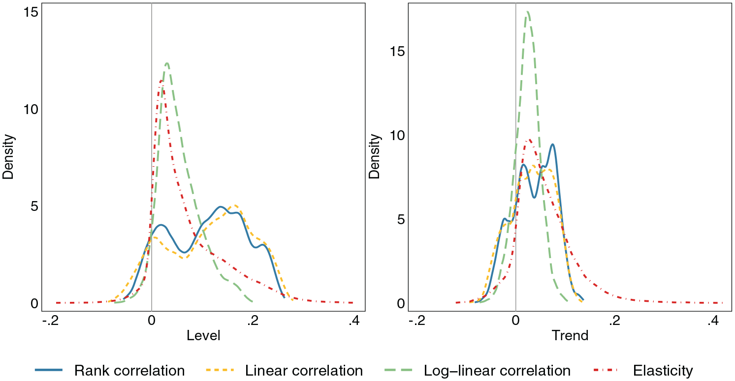
Levels and Trends in Intergenerational Associations

What is the upper bound of intergenerational income associations in Sweden? The elasticity has a higher upper bound: .41 versus .26 and .28 for rank and linear correlations, respectively (see Tables A2 to A5 in the online supplement), but the very high elasticities are observed only in a few specifications. The log-linear correlation is both lowest on average and has the lowest upper bound: .20 (Table A4). In the vast majority of cases, we do not reach higher associations than seen in previous literature on Scandinavian countries. A substantial fraction of associations are negative, foremost accounted for by early measurement of child income (i.e., life-cycle bias).

In additional analyses, we expand the observation span to more than 30 years in each generation.⁹ The maximum associations we observe in these analyses all pertain to father/son associations, and are .30 (rank correlation), .33 (linear correlation), .31 (log-linear correlation), and .41 (elasticity) (see Table A6 in the online supplement). This rather low sensitivity to expansion of the observation window is likely to hold in other studies using high-quality tax register data; studies using survey data may be more sensitive to measurement error.

For trends, most estimates point to an increased persistence over time. The shape of the distribution is similar to that of levels, although it is more concentrated around zero and somewhat less dispersed (Figure 2, right panel). The elasticity shows steeper trends than do other measures of association (Table A5). This is explained by the rise of inequality, which causes a mechanic increase in the elasticity, as we detail in the Appendix. Although most trend estimates show rising persistence, for all parameters of association and combinations of parent and child sex, there are trends in either direction (see Tables A2 to A5 in the online supplement).

What Explains the Variation?

To unpack which model components exert the most influence on results, we focus on the rank correlation; detailed results for other parameters are presented in the online supplement. We return to the choice of parameter later.

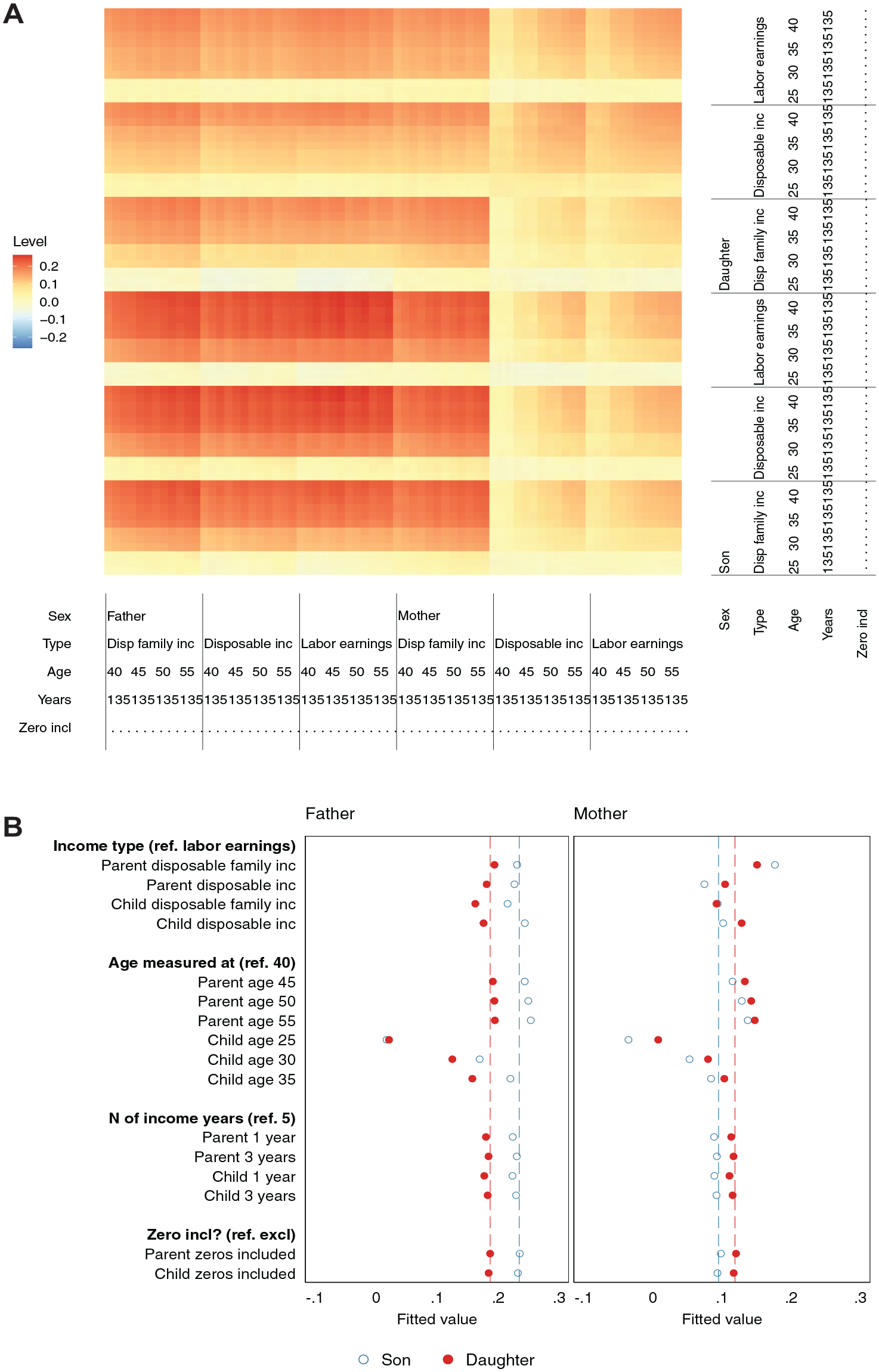
Figure 3 displays how the level of rank correlations varies across 20,736 different specifications defined by parent and child sex, income type, age and observation window, and the treatment of zero values. The top panel (A) displays a heatmap showing the estimated correlation for each specification. The bottom panel (B) focuses separately on each quadrant defined by parent and child sex and shows how remaining model components affect the level of correlation. The markers report coefficient estimates from a linear regression where the level is modeled as a function of income type, age, observation span, and zeros, and fit separately for father/son, father/daughter, mother/son, and mother/daughter pairs.

Figure 3.

Intergenerational Rank Correlation: Variation in Levels

Which model components matter most for the level of rank correlations? Focusing on Figure 3, panel (A), two dimensions stand out: the child’s age at measurement and the sex of both the parent and the child. Intergenerational correlations measured when the child is 25 are close to zero and in some cases negative. This is the well-known life-cycle bias (Haider and Solon 2006): children from advantaged origins spend longer in schooling and experience steeper earnings growth, so they will have low earnings early in their careers. Dropping incomes at age 25 eliminates negative associations in our data (see Figure A3 in the online supplement).

However, age at measurement also exerts a clear influence later in one’s career, and correlations grow gradually stronger at 30, 35, and 40 years of age. This contradicts the notion, made popular by Chetty and colleagues (2014a), that the rank correlation reduces the need for mature incomes. In fact, child age is the single most important predictor of variation in levels (see Table A8 in the online supplement), but again less so when focusing solely on income at age 30 or above (see Table A12).

After child age, the most influential components in Figure 3 are parent sex, parent income type, child sex, child income type, and parent age (see Table A8). Notably, the number of income years observed in either generation and the exclusion of zero incomes are inconsequential for rank correlations (but not for log-based measures, which we discuss below). As for the sex of parent and offspring, father/son correlations are strongest, followed by father/daughter, mother/daughter, and finally mother/son correlations, which are the weakest.

Correlations involving mothers’ incomes become more similar to those of fathers when using family income, which is unsurprising as this includes fathers’ incomes in most households. Notably, correlations increase sharply with mothers’ age. This points to the later maturation of women’s income careers and the risk of underestimating the role of mothers if applying an analytic template optimized for the typical career pattern of men.

Which choices affect the trend in estimated rank correlations? Figure 4 follows the same logic as Figure 3 but now showing how the trend over a 20-year period depends on various components. As we saw in Figure 2, most specifications show a trend toward increasing persistence. Figure 4 shows that the dimensions that predict trends are largely the same as those that predict levels: age, sex, and income type—although the child’s sex and income type matter more for trends, whereas the parent’s sex and income type are more important for levels (see Table A8 in the online supplement). The trend toward increased persistence is mostly absent at young child ages. This may be explained by the increasing average length of schooling over the period, such that earnings differences are realized increasingly late in one’s career.

Figure 4.

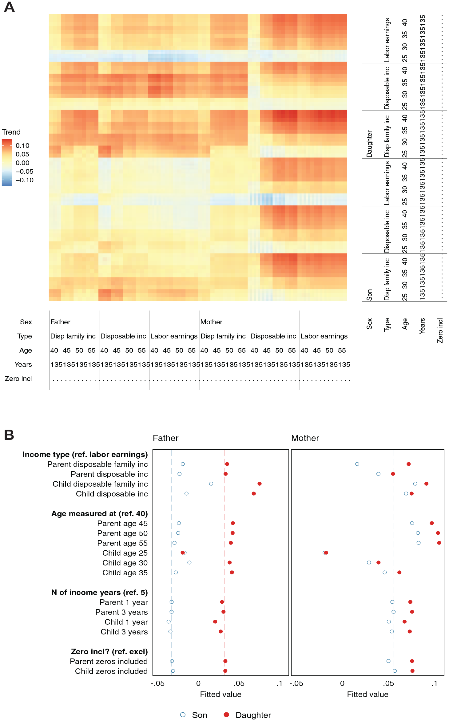
Intergenerational Rank Correlation: Variation in Trends

A notable pattern in Figure 4 is that most of the specifications that show increased persistence contain either mothers or daughters. In fact, comparing Figures 3 and 4 reveals that correlations between fathers and sons, or mothers’ family income and sons, both show the highest level of correlation and either no trend or one toward weakening persistence. By contrast, focusing on the quadrants involving mothers and daughters, correlations are weaker at baseline but rise over time. We now turn to the role of women in these shifts over time.

The Changing Role of Women

One upshot of our analysis is that women’s earnings, either directly or indirectly (as a component of family income), are the predominant driver of increased persistence. Figure 5 shows trends in rank correlations separately by income type and parent and child sex. The male earnings correlation remains flat or slightly decreases, whereas the correlation between father family income and son earnings sees a weak increase in persistence. For all other curves, there is a clear trend of increasing persistence over time.

Figure 5.

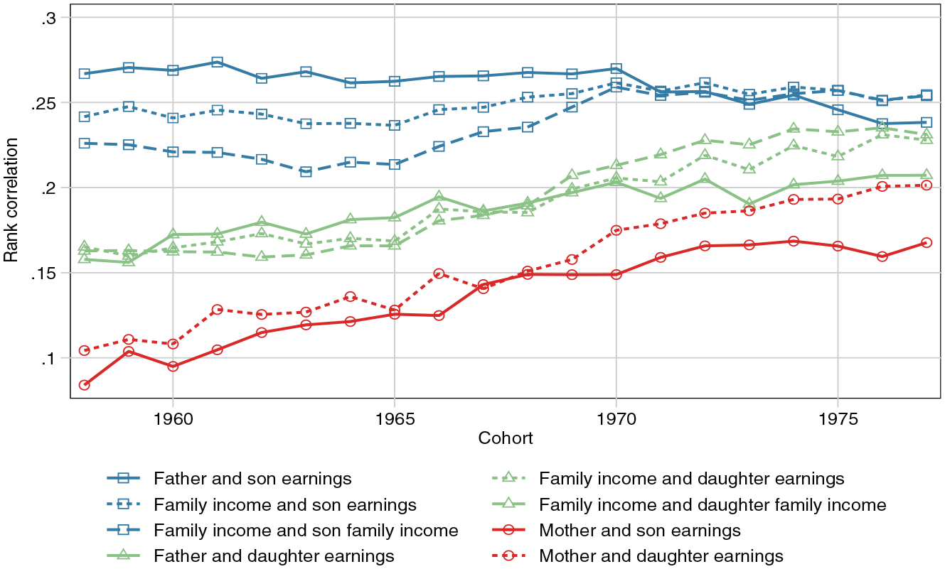
Intergenerational Rank Correlation by Sex and Income Type

To gain a more thorough understanding of the role of women, we return to our theoretical model in Figure 1. That women’s earnings drive increased persistence could mean several things. Women’s rising earnings may contribute to rising inequality between households and thereby unequal investments in children. Such a pattern would depend on the degree of assortative mating. Another possibility is that we have seen a strengthening of the paths from women’s assets to rewards, in the vocabulary of Figure 1.

We first consider the unequal investments pathway. In general, female labor market participation tends to go together with decreasing, not increasing, inequality between families (Harkness 2013; Lam 1997; Mastekaasa and Birkelund 2011; Nieuwenhuis, Van der Kolk, and Need 2017; Rosche 2022), and assortative mating contributes little to inequality between households (Boertien and Bouchet-Valat 2022). In Sweden, assortative mating has decreased or been largely stable (Henz and Jonsson 2003; Holmlund 2022), and income inequality was at its lowest point during the 1980s, when the youngest cohorts in our study grew up. Hence, potential childhood investments grew more equal over these cohorts, so inequality is unlikely to be driving increased persistence. Moreover, such an explanation cannot account for the strikingly different trends we see for daughters and sons.

A more plausible explanation is increased gender equality in the labor market, through a narrowing wage gap or increased female labor supply (Gonalons-Pons and Schwartz 2017). In Figure 6, we show that over our studied cohorts, education has gone from explaining 7 to 8 percent of the variance in women’s earnings ranks, to explaining 17 to 21 percent (the lower number is for level of education, the higher number for a combination of level and field). Among men, the change is in the opposite direction but smaller: from 17–18 to 14–17 percent. At the same time, fathers’ earnings percentile has had a stable, or slightly decreasing, power to predict whether or not a child gets a university education. In other words, the changing trends in mobility that we find for women and family income do not reflect changing investments in children, but rather the extent to which women’s earnings mirror their underlying human capital.

Figure 6.

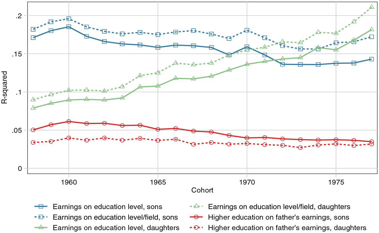
Trends in Returns to and Social Selection into Education

Rank Correlation versus Other Parameters

So far, we have focused on the rank correlation; we now examine differences between all four parameters of association. The rank correlation was popularized in work using U.S. tax data, where the elasticity has been difficult to estimate due to limited observation spans (Chetty et al. 2014a). Many scholars maintain that the elasticity remains theoretically preferred when data quality does not hinder its use (Mazumder 2016; Mitnik et al. 2019; Mitnik and Grusky 2020). Some work has compared how these measures are affected by measurement error and life-cycle biases (Nybom and Stuhler 2017). We know less about how sensitive trends are, and whether this might differ across parameters.

To condense information about levels and trends, we plot estimates for all four measures in Figure 7, where each dot represents a specification. Detailed results for the linear correlation, log-linear correlation, and elasticity are available in Figures A4 to A9 in the online supplement. The first thing that stands out is that linear correlations show a near-identical pattern to rank correlations: estimates from these two measures correlate at r = .99 across specifications (see Table A7). This follows from the linear correlation providing a good fit in our data: whenever standard normality assumptions are satisfied, linear and rank correlations are by definition closely linked (see the Appendix).

Figure 7.

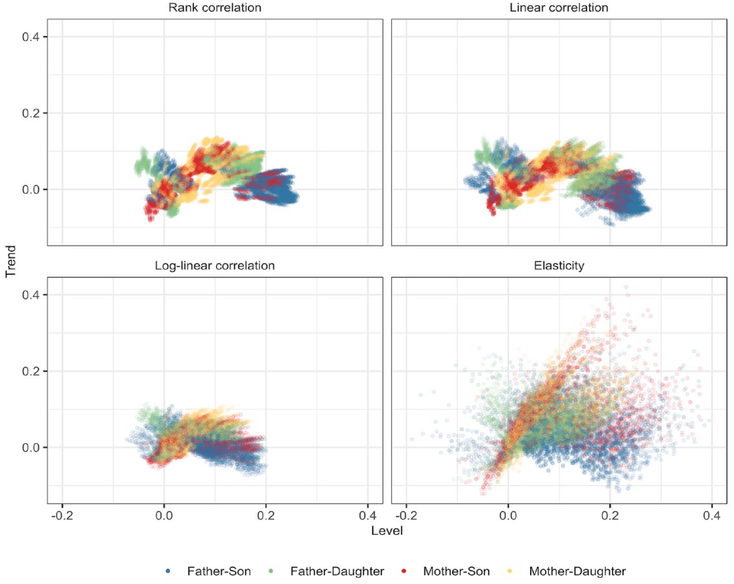
Correlation between Level and Trend in Intergenerational Associations

The log-linear correlation differs from rank and linear correlations in two respects. The level of the correlation is lower, and the estimates are clustered more tightly together, without showing the same clear patterning by parent and child sex. While this might suggest log-linear correlations are in one sense more “robust,” it is not clear this invariance is a good thing if specifications speak to different questions. The elasticity equals the log-linear correlation multiplied by the ratio of standard deviations in parent and child income (see the Appendix). It shows a wider dispersion in both levels and trends. This could be driven, in part, by specifications with different income definitions on the parent and child side, which should differ in dispersion. However, the picture looks similar when we restrict ourselves to specifications that treat income symmetrically on each side (see Figure A11 in the online supplement).

What components account for variation in the log-based measures? The same components tend to matter for the level of estimated associations, and in similar ways, as for the rank or linear correlation. The main exception is that log-based measures are more sensitive to the number of income years and, particularly, the treatment of zeros, which in our data make up less than 3 percent in all groups but mothers (see Table A13 in the online supplement).¹⁰ This sensitivity to low values suggests the functional form may provide a poor fit to data. We examine the model fit directly in Figure A12 and confirm that the log functional form overfits low values and performs poorly in the upper half of the distribution. In other words, using log-based measures amounts to a judgment that the upper half of the distribution is of less weight, and should be treated as a substantive choice.

Do different measures tell the same story about trends? The agreement is lower for trends than it is for levels (see Table A7 in the online supplement). In other words, whereas most model components have a similar influence on the level, this is not true for trends: the choices that matter for log-based measures differ from those that influence rank or linear correlations.¹¹ For some choices, the influence is the opposite across different parameters. For example, measuring income at high father ages increases the trend in the rank correlation but decreases that in the log-linear correlation or elasticity (see Figures A8 and A9 in the online supplement). For all four measures of association, variation in trends is less systematic than that in levels. While the bulk of variation in levels is explained by the main effects of individual model ingredients, trends depend to a higher extent on two-way or higher-order interactions that are hard to predict or interpret (Tables A8 to A11).

Where does this leave us with respect to the debate on the relative merits of rank correlations and log-based measures? The rank correlation, as well as the linear one, fits the data closely and picks up systematic patterns of variation that are easier to miss with log-based measures that behave more erratically. Elasticities and log-linear correlations are sensitive to a number of additional dimensions and have a tendency to overfit the bottom of the distribution. This extreme dependence is apparent in Figure 8, which shows a wide range of levels and trends depending on the treatment of a small number of zeros among men in our data. Even with the kind of high-quality data we have access to here—prime ages, high coverage, long time-spans—it is difficult to recommend log-based measures as a reliable basis for inference about income mobility.

Figure 8.

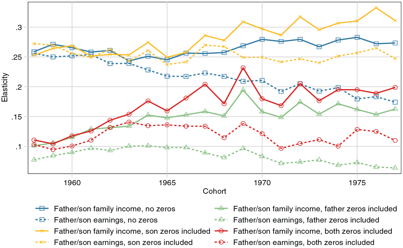
Intergenerational Elasticity by Treatment of Zeros and Income Type, Men

Conclusions

The social sciences are currently undergoing a credibility crisis, or credibility revolution, depending on whom you ask (Engzell and Rohrer 2021). There is growing awareness of how the many and varied options faced by an analyst can lead to selective reporting that risks systematically biasing a literature. Each analytical choice may seem trivial or innocuous on its own, but they accumulate into a proverbial “garden of forking paths,” allowing a researcher to pick almost any desired result (Gelman and Loken 2014). The field of income mobility research is no exception: given the variety of specifications and lack of general guidelines, this area would seem like a paradigm case of forking paths. To shed light on this issue, we applied multiverse analysis, which maps variation across specifications to bring model dependency out in the open.

We demonstrated how this tool can be used not only to gauge robustness, but also—with an abductive logic of inference—to shift our theoretical understanding of the phenomenon studied. Selecting a given specification to test a prediction such as “mobility is declining,” we would have been likely to confirm it. By contrast, examining the full model space we can begin to address questions not only of if but why. In our case, the striking conclusion is that rising gender equality, not inequality, is the main driver of declining income mobility in Sweden today. Intergenerational correlations rise over time because women’s earnings become a better proxy for their underlying human capital, and this also influences family income. Our results show that rising intergenerational persistence can be a result of something most would see as desirable: gender equalization in the labor market.

The implication for mobility research is that it must go from merely acknowledging gender to placing it center stage. Women’s rising earnings will affect not only women themselves, but also the men they share families and labor markets with. This is a force powerful enough to be the main driver of trends and differences across countries, and it cannot be ignored. More generally, our results draw attention to the broader role of labor market processes in intergenerational stratification. Work in this area has focused on early-life investments and ignored the relative pay of different segments of the labor market. Arguably, this research would benefit from tighter integration with literature on the sources of earnings inequality in the labor market. Work parallel to ours confirms the importance for mobility analyses of considering characteristics of labor markets (Deutscher and Mazumder forthcoming; Engzell and Wilmers 2023; Granström and Engzell 2023) and women’s earnings (Ahrsjö, Karadakic, and Rasmussen 2023; Brandén, Nybom, and Vosters 2023).

Another observation is that variation is very large even for a given measure of association, and for a given combination of parent and child sex. For example, the rank correlation, which is generally taken to be the most robust measure of association, spans from weakly negative to around .30 for the father/son-combination, using different reasonable specifications. This large variation means that researcher degrees of freedom can give rise to varying conclusions. For instance, some prior work on Scandinavia has reported rising persistence (Hansen 2010; Harding and Munk 2020; Pekkala and Lucas 2007; Wiborg and Hansen 2018), yet other work finds conflicting results (Bratberg Nilsen, and Vaage 2005; Jonsson et al. 2011; Pekkarinen et al. 2017). This variation is hardly surprising in light of our analysis, as it is easy to reach conflicting conclusions about trends even with the same dataset—sometimes due to seemingly arbitrary choices of specification.

How should applied researchers tackle this staggering variation? A multiverse analysis may not be the appropriate course to take for all research projects. But arguably it should be incorporated as a standard tool among others. The form that a given multiverse analysis takes must depend on the specific purpose and theory. If the question is precise and all specifications can reasonably be seen as approximating the same underlying concept, a researcher may proceed with methods such as model averaging to arrive at more robust estimates. In practice, however, this will seldom be the case, and a more reasonable approach will be to display a range of estimates. Ideally, theory can lead us to agree on specifications that are more or less practical, but even so, the chase for a single “best” estimate may be misplaced.

It is worth distinguishing the idea of robustness from variation that is more substantively or theoretically grounded. However, as we argued, a sharp line can be difficult to draw a priori and will often have to arise from the data at hand. In fact, even choices that are motivated by certain theoretical considerations might turn out to have quite different implications once confronted with data. Take elasticities, motivated by a model rooted in human capital theory (Becker and Tomes 1986). The motivation may be sound, but it is of little worth if the data are at odds with the resulting functional form. In this case, the log transform turns out to put disproportionate weight on cases in the bottom of the distribution. This itself amounts to a substantive judgment that movements in the bottom of the distribution are of greater interest than those in the upper half.

We placed particular focus on the rank correlation, given its increasing popularity and its apparent promise in terms of robustness. On the one hand, the rank correlation is less sensitive to some choices—the number of years income is observed and the treatment of zeros—that can have a large influence on log-based measures such as the elasticity. On the other hand, it remains heavily influenced by child age and income type. Regarding age, we find that measuring income at age 25 gives rank correlations that are close to zero and for later cohorts even negative. Although age 25 is younger than best practices would recommend, the fact that inclusion of these early incomes affects both levels and trends is notable, as researchers have assumed trends would be unaffected (Chetty et al. 2014b). Age remains an important predictor of levels and trends in rank correlations, with clear differences also between the more mature ages of 35 and 40. Although our results cannot be generalized beyond the Swedish setting, they show that rank correlations do not allow researchers to drop their guard against life-cycle bias.

The literature on intergenerational income mobility often seems like a flurry of numbers, and in this article we contribute quite a few more. Our goal, however, has been to anchor all these numbers in a systematic framework so that differences between them can become a source of information rather than a source of confusion. Model dependency is a very real challenge to the field, but we believe it is a challenge we can rise to in productive ways. Most importantly, variation in estimates along systematic lines should spur researchers to sharpen their questions: “How large is intergenerational economic persistence?” is an important question, yet a vague one. Much time and energy have been spent on the chase for the one best estimate (.3, .6, or perhaps .42?), but this chase for a “best specification” is futile if there is no stable target: if different measures of economic resources to a large extent proxy for different underlying factors, they cannot be treated as interchangeable.

By embracing variation and using an abductive approach, what now sometimes seems like a jumble of numbers can be transformed into informative patterns. Patterns, however, do not always form neat narratives. As we have shown, a lot of variation—particularly in trends—is seemingly unsystematic. Moreover, even with a clear target concept, many operationalizations will seem equally reasonable, and even good data put limits to what can be achieved. With steadily expanding high-quality data and computational power, the field is ready for a more systematic incorporation of variability through multiverse estimation. Accumulation of multimodel evidence from various sources will increase transparency and credibility, and holds promise for theoretical progress not just in intergenerational mobility research, but across a wide range of fields.

Supplemental Material

sj-pdf-1-asr-10.1177_00031224231180607 – Supplemental material for Understanding Patterns and Trends in Income Mobility through Multiverse Analysis

Supplemental material, sj-pdf-1-asr-10.1177_00031224231180607 for Understanding Patterns and Trends in Income Mobility through Multiverse Analysis by Per Engzell and Carina Mood in American Sociological Review

Footnotes

Appendix: Measures Of Intergenerational Mobility

The literature on economic mobility has generated a variety of measures. Recent research has preferred the rank-order correlation, also known as Spearman’s ρ and equivalent to Pearson’s r if each variable is transformed to percentile ranks:

(1)

\begin{array}{l} ρ = C o r r (R [y_{t}], R [y_{t - 1}]) \\ = \frac{C o v (R [y_{t}], R [y_{t - 1}])}{\sqrt{V a r (R [y_{t}])} \sqrt{V a r (R [y_{t - 1}])}}, \end{array}

where y_t−1 and y_t denote parent and child income and R ∈ {1, 2, . . ., 100} represents the rank transform. The second measure we examine is the linear correlation, or Pearson’s r, imposing no transformation on incomes other than top-coding of extreme outliers (four standard deviations above the mean). This measure can be written as follows:

(2)

r = C o r r (y_{t}, y_{t - 1}) = \frac{C o v (y_{t}, y_{t - 1})}{\sqrt{V a r (y_{t})} \sqrt{V a r (y_{t - 1})}}

In practice, we find that the rank correlation and the linear correlation behave similarly. This follows from the fact that the linear correlation provides a good fit in the Swedish data. In fact, with a bivariate normal distribution, there is a precise mathematical relationship between ρ and r (Pearson 1907):

(3)

ρ = \frac{6}{π} \arcsin (\frac{r}{2}), r = 2 \sin (\frac{π}{6} ρ)

Plotting this function reveals a near-linear dependency (see Figure A1 in the online supplement). This means that for the bivariate normal case, ρ and r are bound to be almost identical. More commonly, researchers tend to log transform incomes whenever the rank transform is not used. This leads to one of two measures: the log-linear correlation or the intergenerational elasticity. We denote the log-linear correlation ϕ following Fox, Torche, and Waldfogel (2016), and the intergenerational elasticity β as conventional. The definition of ϕ follows that of Pearson’s r above, except income is transformed to its natural logarithm:

(4)

\begin{array}{l} φ = C o r r (\ln y_{t}, \ln y_{t - 1}) \\ = \frac{C o v (\ln y_{t}, \ln y_{t - 1})}{\sqrt{V a r (\ln y_{t})} \sqrt{V a r (\ln y_{t - 1})}} \end{array}

Finally, the elasticity β reflects the derivative of expected log child income with respect to log parent income. As a regression coefficient, it is identical to ϕ with the exception that it does not normalize by the ratio of standard deviations in each generation, and hence depends on the marginal distributions of parent and child income:

(5)

\begin{array}{l} β = \frac{C o v (\ln y_{t}, \ln y_{t - 1})}{\sqrt{V a r (\ln y_{t - 1})}} \\ = C o r r (\ln y_{t}, \ln y_{t - 1}) \frac{\sqrt{V a r (\ln y_{t})}}{\sqrt{V a r (\ln y_{t - 1})}} \end{array}

In particular, if the dispersion of y increases from t − 1 to t, the ratio $\sqrt{V a r (\ln y_{t})} / \sqrt{V a r (\ln y_{t - 1})}$ will increase and so will the estimated coefficient. In other words, there is a mechanical dependence where, if income inequality follows a rising trend over time, all else equal, the elasticity will be larger.

Acknowledgements

A previous version of this paper was circulated under the title “How Robust Are Estimates of Intergenerational Income Mobility?” It has benefited from presentations at the 2019 MZES Open Social Science Conference in Mannheim, the 2019 ECSR Annual Conference in Lausanne, and seminars at the UCL Social Research Institute, University College London; Centre for Economic Demography, Lund University; Department of Sociology and Human Geography, University of Oslo; Institute for Sociology, Ludwig Maximilian University of Munich; the Joint Research Centre of the European Commission; the Norwegian University of Science and Technology; and the Center for Advanced Social Science Research, New York University. For comments that greatly improved the paper, we thank the editors and anonymous reviewers at American Sociological Review, members of the editorial team at Sociological Science, as well as Richard Breen, Elien van Dongen, Jeremy Freese, Martin Hällsten, Jan O. Jonsson, Lindsey Macmillan, Saul Justin Newman, Therese Nilsson, Charles Rahal, Shiva Rouhani, Max Thaning, and Nathan Wilmers. Any errors remain our own.

Funding

This work was supported by Swedish Research Council for Health, Working Life and Welfare (Forte) grant 2016-07099 and the Swedish Research Council (VR) grant 2022-02036.

ORCID iD

Per Engzell

Notes

Per Engzell is Associate Professor of Sociology at UCL Social Research Institute, University College London, Associate Member of Nuffield College, University of Oxford, and Docent at the Swedish Institute for Social Research (SOFI), Stockholm University. His research interests include intergenerational mobility and educational stratification.

Carina Mood is Professor of Sociology at the Swedish Institute for Social Research (SOFI), Stockholm University. Her research interests cover poverty, social inequality, intergenerational mobility, and integration. She is co-PI of the Swedish Level-of-Living Surveys and the Swedish CILS4EU project.

References

Aaronson

Daniel

Mazumder

Bhashkar

. 2008. “Intergenerational Economic Mobility in the United States, 1940 to 2000.” Journal of Human Resources 43(1):139–72.

Ahrsjö

Ulrika

Karadakic

René

Rasmussen

Joachim Kahr

. 2023. “Intergenerational Mobility Trends and the Changing Role of Female Labor.” arXiv preprint (https://doi.org/10.48550/arXiv.2302.14440).

Andersson

Gunnar

Duvander

Ann-Zofie

Hank

Karsten

. 2004. “Do Child-Care Characteristics Influence Continued Child Bearing in Sweden? An Investigation of the Quantity, Quality, and Price Dimension.” Journal of European Social Policy 14(4):407–18.

Baron, James N., and William T. Bielby . 1980. “Bringing the Firms Back In: Stratification, Segmentation, and the Organization of Work.” American Sociological Review 45(5):737–65.

Becker

Gary S.

Tomes

Nigel

. 1979. “An Equilibrium Theory of the Distribution of Income and Intergenerational Mobility.” Journal of Political Economy 87(6):1153–89.

Becker

Gary S.

Tomes

Nigel

. 1986. “Human Capital and the Rise and Fall of Families.” Journal of Labor Economics 4(3):S1–S39.

Beller

Emily

. 2009. “Bringing Intergenerational Social Mobility Research into the Twenty-First Century: Why Mothers Matter.” American Sociological Review 74(4):507–28.

Berk

Richard

Brown

Lawrence

Zhao

Linda

. 2010. “Statistical Inference after Model Selection.” Journal of Quantitative Criminology 26(2):217–36.

Björklund

Anders

Jäntti

Markus

. 1997. “Intergenerational Income Mobility in Sweden Compared to the United States.” American Economic Review 87(5):1009–18.

10.

Björklund

Anders

Jäntti

Markus

Lindquist

Matthew J.

2009. “Family Background and Income during the Rise of the Welfare State: Brother Correlations in Income for Swedish Men Born 1932–1968.” Journal of Public Economics 93(5):671–80.

11.

Bloome

Deirdre

. 2015. “Income Inequality and Intergenerational Income Mobility in the United States.” Social Forces 93(3):1047–80.

12.

Bloome

Deirdre

Dyer

Shauna

Zhou

Xiang

. 2018. “Educational Inequality, Educational Expansion, and Intergenerational Income Persistence in the United States.” American Sociological Review 83(6):1215–53.

13.

Boertien

Diederik

Bouchet-Valat

Milan

. 2022. “Are Increasing Earnings Associations between Partners of Concern for Inequality? A Comparative Study of 21 Countries.” Social Forces 101(2):639–64.

14.

Brandén

Gunnar

Nybom

Martin

Vosters

Kelly

. 2023. “Like Mother, Like Child? The Rise of Women’s Intergenerational Income Persistence in Sweden and the United States.” Presented at the 2023 Annual Meeting of the Society of Labor Economists, Philadelphia, May 12–13.

15.

Brandt

Philipp

Timmermans

Stefan

. 2021. “Abductive Logic of Inquiry for Quantitative Research in the Digital Age.” Sociological Science 8:191–210.

16.

Bratberg

Espen

Nilsen

Øivind Anti

Vaage

Kjell

. 2005. “Intergenerational Earnings Mobility in Norway: Levels and Trends.” Scandinavian Journal of Economics 107(3):419–35.

17.

Bratberg

Espen

Nilsen

Øivind Anti

Vaage

Kjell

. 2007. “Trends in Intergenerational Mobility across Offspring’s Earnings Distribution in Norway.” Industrial Relations 46(1):112–29.

18.

Bratsberg

Bernt

Røed

Knut

Raaum

Oddbjørn

Naylor

Robin

Jäntti

Markus

Eriksson

Tor

Österbacka

Eva

. 2007. “Nonlinearities in Intergenerational Earnings Mobility: Consequences for Cross-Country Comparisons.” Economic Journal 117(519):C72–C92.

19.

Breen

Richard

Jonsson

Jan O.

2005. “Inequality of Opportunity in Comparative Perspective: Recent Research on Educational Attainment and Social Mobility.” Annual Review of Sociology 31:223–43.

20.

Breen

Richard

Jonsson

Jan O.

2007. “Explaining Change in Social Fluidity: Educational Equalization and Educational Expansion in Twentieth-Century Sweden.” American Journal of Sociology 112(6):1775–810.

21.

Carneiro

Pedro

García

Italo López

Salvanes

Kjell G.

Tominey

Emma

. 2021. “Intergenerational Mobility and the Timing of Parental Income.” Journal of Political Economy 129(3):757–88.

22.

Chadwick

Laura

Solon

Gary

. 2002. “Intergenerational Income Mobility among Daughters.” American Economic Review 92(1):335–44.

23.

Chang

Yoosoon

Durlauf

Steven N.

Lee

Seunghee

Park

Joon Y.

2023. “A Trajectories-Based Approach to Measuring Intergenerational Mobility.” National Bureau of Economic Research, Working Paper No. w31020.

24.

Charles

Maria

. 2011. “A World of Difference: International Trends in Women’s Economic Status.” Annual Review of Sociology 37:355–71.

25.

Chen

Wen-Hao

Ostrovsky

Yuri

Piraino

Patrizio

. 2017. “Lifecycle Variation, Errors-in-Variables Bias and Nonlinearities in Intergenerational Income Transmission: New Evidence from Canada.” Labour Economics 44(1):1–12.

26.

Cheng

Siwei

Song

. 2019. “Linked Lives, Linked Trajectories: Intergenerational Association of Intragenerational Income Mobility.” American Sociological Review 84(6):1037–68.

27.

Chetty

Raj

Hendren

Nathaniel

Kline

Patrick

Saez

Emmanuel

. 2014a. “Where Is the Land of Opportunity? The Geography of Intergenerational Mobility in the United States.” Quarterly Journal of Economics 129(4):1553–623.

28.

Chetty

Raj

Hendren

Nathaniel

Kline

Patrick

Saez

Emmanuel

Turner

Nicholas

. 2014b. “Is the United States Still a Land of Opportunity? Recent Trends in Intergenerational Mobility.” American Economic Review 104(5):141–47.

29.

Choi

Seongsoo

Chung

Inkwan

Breen

Richard

. 2020. “How Marriage Matters for the Intergenerational Mobility of Family Income: Heterogeneity by Gender, Life Course, and Birth Cohort.” American Sociological Review 85(3):353–80.

30.

Corak

Miles

. 2006. “Do Poor Children Become Poor Adults? Lessons from a Cross-Country Comparison of Generational Earnings Mobility.” Research on Economic Inequality 13(1):143–88.

31.

Corak

Miles

. 2013. “Income Inequality, Equality of Opportunity, and Intergenerational Mobility.” Journal of Economic Perspectives 27(3):79–102.

32.

Corak

Miles

Heisz

Andrew

. 1999. “The Intergenerational Earnings and Income Mobility of Canadian Men: Evidence from Longitudinal Income Tax Data.” Journal of Human Resources 34(3):504–33.

33.

Dahl

Molly W.

DeLeire

Thomas

. 2008. “The Association between Children’s Earnings and Fathers’ Lifetime Earnings: Estimates Using Administrative Data.” University of Wisconsin–Madison, Institute for Research on Poverty, Discussion Paper No. 1342-08.

34.

Davis

Jonathan

Mazumder

Bhashkar

. 2020. “The Decline in Intergenerational Mobility after 1980.” City University of New York, Stone Center on Socio-Economic Inequality, Working Paper No. 11.

35.

Deutscher

Nathan

Mazumder

Bhashkar

. Forthcoming. “Measuring Intergenerational Income Mobility: A Synthesis of Approaches.” Journal of Economic Literature.

36.

Engzell

Per

Rohrer

Julia M.

2021. “Improving Social Science: Lessons from the Open Science Movement.” PS: Political Science & Politics 54(2):297–300.

37.

Engzell

Per

Wilmers

Nathan

. 2023. “Firms and the Intergenerational Transmission of Labor Market Advantage.” SocArXiv ( https://doi.org/10.31235/osf.io/mv3e9).

38.

Ermisch

John

Jäntti

Markus

Smeeding

Timothy

Wilson

James A.

2018. “Advantage in Comparative Perspective.” Pp. 501–505 in Social Stratification, 4th ed., edited by Grusky

D. B.

Weisshaar

K. R.

New York: Routledge.

39.

Eshaghnia

Sadegh

Heckman

James J.

Landersø

Rasmus

. 2023. “Maximum Impact Intergenerational Associations.” National Bureau of Economic Research, Working Paper No. w31093.

40.

Fertig

Angela R.

2003. “Trends in Intergenerational Earnings Mobility in the United States.” Journal of Income Distribution 12(3–4):108–30.

41.

Forslund

Anders

. 2008. “Den svenska jämviktsarbetslösheten: En översikt.”

42.

Institute for Evaluation of Labour Market and Education Policy (IFAU), Report 2008:17.

43.

Fox

Liana

Torche

Florencia

Waldfogel

Jane

. 2016. “Intergenerational Mobility.” In Oxford Handbook of the Social Science of Poverty, edited by Brady

Burton

L. M.

Oxford, UK: Oxford University Press.

44.

Freedman

David A.

1991. “Statistical Models and Shoe Leather.” Sociological Methodology 21:291–313.

45.

Freese

Jeremy

Rauf

Tamkinat

Voelkel

Jan Gerrit

. 2022. “Advances in Transparency and Reproducibility in the Social Sciences.” Social Science Research 107 (https://doi.org/10.1016/j.ssresearch.2022.102770).

46.

Gähler

Michael

Palmtag

Eva-Lisa

. 2015. “Parental Divorce, Psychological Well-Being and Educational Attainment: Changed Experience, Unchanged Effect among Swedes Born 1892–1991.” Social Indicators Research 123(2):601–23.

47.

Gelman

Andrew

Loken

Eric

. 2014. “The Statistical Crisis in Science.” American Scientist 102(6):460–66.

48.

Goldin

Claudia

. 2006. “The Quiet Revolution That Transformed Women’s Employment, Education, and Family.” American Economic Review 96(2):1–21.

49.

Gonalons-Pons

Pilar

Schwartz

Christine R.

2017. “Trends in Economic Homogamy: Changes in Assortative Mating or the Division of Labor in Marriage?” Demography 54(3):985–1005.

50.

Granström

Olivia

Engzell

Per

. 2023. “The Geography of Intergenerational Mobility in Europe.” SocArXiv (https://doi.org/10.31235/osf.io/gzwha).

51.

Gregg

Paul

Jonsson

Jan O.

Macmillan

Lindsey

Mood

Carina

. 2017. “The Role of Education for Intergenerational Income Mobility: A Comparison of the United States, Great Britain, and Sweden.” Social Forces 96(1):121–52.

52.

Gregg

Paul

Macmillan

Lindsey

. 2020. “Intergenerational Joblessness across Europe: The Role of Labour Markets, Education, and Welfare Generosity.” UCL Centre for Education Policy and Equalising Opportunities, CEPEO Working Paper 20-11.

53.

Gregg

Paul

Macmillan

Lindsey

Vittori

Claudia

. 2017. “Moving towards Estimating Sons’ Lifetime Intergenerational Economic Mobility in the UK.” Oxford Bulletin of Economics and Statistics 79(1):79–100.

54.

Griffen

Zachary W.

2023. “The Economization of Early Life: Human Capital Theory, Biology, and Social Policy.” Science, Technology, & Human Values (https://doi.org/10.1177/01622439221147701).

55.

Grusky

David B.

Szelenyi

Szonja

. 2018. “The Stories We Tell about Inequality.” Pp. 17–25 in Social Stratification, 4th ed., edited by Grusky

D. B.

Weisshaar

K. R.

New York: Routledge.

56.

Haack

Susan

. 2000. Manifesto of a Passionate Moderate: Unfashionable Essays. Chicago: University of Chicago Press.

57.

Haider

Steven

Solon

Gary

. 2006. “Life-Cycle Variation in the Association between Current and Lifetime Earnings.” American Economic Review 96(4):1308–20.

58.

Hansen

Marianne N.

2010. “Change in Intergenerational Economic Mobility in Norway: Conventional versus Joint Classifications of Economic Origin.” Journal of Economic Inequality 8(2):133–51.

59.

Hansen

Marianne N.

Toft

Maren

. 2021. “Wealth Accumulation and Opportunity Hoarding: Class-Origin Wealth Gaps over a Quarter of a Century in a Scandinavian Country.” American Sociological Review 86(4):603–38.

60.

Harding

David J.

Munk

Martin D.

2020. “The Decline of Intergenerational Income Mobility in Denmark: Returns to Education, Demographic Change, and Labor Market Experience.” Social Forces 98(4):1436–64.

61.

Harkness

Susan

. 2013. “Women’s Employment and Household Income Inequality.” Pp. 207–233 in Income Inequality: Economic Disparities and the Middle Class in Affluent Countries, edited by Gornick

J. C.

Jäntti

Stanford, CA: Stanford University Press.

62.

Härkönen

Juho

Bihagen

Erik

. 2011. “Occupational Attainment and Career Progression in Sweden.” European Societies 13(3):451–79.

63.

Härkönen

Juho

Manzoni

Anna

Bihagen

Erik

. 2016. “Gender Inequalities in Occupational Prestige across the Working Life: An Analysis of the Careers of West Germans and Swedes Born from the 1920s to the 1970s.” Advances in Life Course Research 29:41–51.

64.

Hederos

Karin

Jäntti

Markus

Lindahl

Lena

. 2017. “Gender and Inequality of Opportunity in Sweden.” Social Choice and Welfare 49(3):605–35.

65.

Henz

Ursula

Jonsson

Jan O.

2003. “Who Marries Whom in Sweden?” Pp. 235–66 in Who Marries Whom? edited by Blossfeld

H.-P.

Timm

Dordrecht: Springer.

66.

Hertz

Tom

. 2007. “Trends in the Intergenerational Elasticity of Family Income in the United States.” Industrial Relations 46(1):22–50.

67.

Hirschman

Daniel

. 2021. “Rediscovering the 1%: Knowledge Infrastructures and the Stylized Facts of Inequality.” American Journal of Sociology 127(3):739–86.

68.

Holmlund

Helena

. 2022. “How Much Does Marital Sorting Contribute to Intergenerational Socioeconomic Persistence?” Journal of Human Resources 57(2):372–99.

69.

Hout

Michael

. 1988. “More Universalism, Less Structural Mobility: The American Occupational Structure in the 1980s.” American Journal of Sociology 93(6):1358–400.

70.

Hout

Michael

. 2018. “Americans’ Occupational Status Reflects the Status of Both of Their Parents.” Proceedings of the National Academy of Sciences 115(38):9527–32.

71.

Hwang

Philip

Broberg

Anders G.

2014. “The Historical and Social Context of Child Care in Sweden.” Pp. 45–72 in Child Care in Context: Cross-Cultural Perspectives, edited by Lamb

M. E.

Sternberg

K. J.

Hwang

C.-P.

Broberg

A. G.

London, UK: Psychology Press.

72.

Jenkins

Stephen

. 1987. “Snapshots versus Movies: ‘Lifecycle Biases’ and the Estimation of Intergenerational Earnings Inheritance.” European Economic Review 31(5):1149–58.

73.

Jenkins

Stephen P.

Siedler

Thomas

. 2007. “The Intergenerational Transmission of Poverty in Industrialized Countries.” Chronic Poverty Research Centre, Working Paper No. 75.

74.

Jonsson

Jan O.

Erikson

Robert

. 2007. “Sweden: Why Educational Expansion Is Not Such a Great Strategy for Equality: Theory and Evidence.” Pp. 113–19 in Stratification in Higher Education: A Comparative Study, edited by Shavit

Arum

Gamoran

Stanford, CA: Stanford University Press.

75.

Jonsson

Jan O.

Mood

Carina

Bihagen

Erik

. 2011. “Poverty in Sweden 1991–2007.” Swedish Institute for Social Research (SOFI), Working Paper 10/2011.

76.

Jonsson

Jan O.

Mood

Carina

Bihagen

Erik

. 2016. “Poverty Trends during Two Recessions and Two Recoveries: Lessons from Sweden 1991–2013.” IZA Journal of European Labor Studies 5(1):1–20.

77.

Lam

David

. 1997. “Demographic Variables and Income Inequality.” Pp. 1015–59 in Handbook of Population and Family Economics, edited by Rosenzweig

Stark

Amsterdam: Elsevier.

78.

Landersø

Rasmus

Heckman

James J.

2017. “The Scandinavian Fantasy: The Sources of Intergenerational Mobility in Denmark and the US.” Scandinavian Journal of Economics 119(1):178–230.

79.

Lee

Chul-In

Solon

Gary

. 2009. “Trends in Intergenerational Income Mobility.” Review of Economics and Statistics 91(4):766–72.

80.

Lieberson

Stanley

Horwich

Joel

. 2008. “Implication Analysis: A Pragmatic Proposal for Linking Theory and Data in the Social Sciences.” Sociological Methodology 38:1–50.

81.

Lipton

Peter

. 2003. Inference to the Best Explanation. New York: Routledge.

82.

Lundberg

Ian

Johnson

Rebecca

Stewart

Brandon M.

2021. “What Is Your Estimand? Defining the Target Quantity Connects Statistical Evidence to Theory.” American Sociological Review 86(3):532–65.

83.

Mastekaasa

Arne

Birkelund

Gunn Elisabeth

. 2011. “The Equalizing Effect of Wives’ Earnings on Inequalities in Earnings among Households: Norway 1974–2004.” European Societies 13(2):219–37.

84.

Mayer

Susan E.

1997. What Money Can’t Buy: Family Income and Children’s Life Chances. Cambridge, MA: Harvard University Press.

85.

Mayer

Susan E.

Lopoo

Leonard M.

2005. “Has the Intergenerational Transmission of Economic Status Changed?” Journal of Human Resources 40(1):169–85.

86.

Mazumder

Bhashkar

. 2016. “Estimating the Intergenerational Elasticity and Rank Association in the United States: Overcoming the Current Limitations of Tax Data.” Research in Labor Economics 43:83–129.

87.

Merton

Robert K.

1987. “Three Fragments from a Sociologist’s Notebooks: Establishing the Phenomenon, Specified Ignorance, and Strategic Research Materials.” Annual Review of Sociology 13:1–29.

88.

Mitnik

Pablo A.

Bryant

Victoria

Weber

Michael

. 2019. “The Intergenerational Transmission of Family-Income Advantages in the United States.” Sociological Science 6:380–415.

89.

Mitnik

Pablo A.

Grusky

David B.

2020. “The Intergenerational Elasticity of What? The Case for Redefining the Workhorse Measure of Economic Mobility.” Sociological Methodology 50:47–95.

90.

Mood

Carina

. 2017. “More Than Money: Social Class, Income, and the Intergenerational Persistence of Advantage.” Sociological Science 4:263–87.

91.

Morris

Martina

Western

Bruce

. 1999. “Inequality in Earnings at the Close of the Twentieth Century.” Annual Review of Sociology 25:623–57.

92.

Muller

Seán M.

2010. “Another Problem in the Estimation of Intergenerational Income Mobility.” Economics Letters 108(3):291–95.

93.

Muñoz

John

Young

Cristobal

. 2018. “We Ran 9 Billion Regressions: Eliminating False Positives through Computational Model Robustness.” Sociological Methodology 48:1–33.

94.

Neckerman

Kathryn M.

Torche

Florencia

. 2007. “Inequality: Causes and Consequences.” Annual Review of Sociology 33:335–57.

95.

Nieuwenhuis

Rense

Van der Kolk

Henk

Need

Ariana

. 2017. “Women’s Earnings and Household Inequality in OECD Countries, 1973–2013.” Acta Sociologica 60(1):3–20.

96.

Nybom

Martin

Stuhler

Jan

. 2017. “Biases in Standard Measures of Intergenerational Income Dependence.” Journal of Human Resources 52(3):800–825.

97.

Parolin

Zachary

Schmitt

Rafael Pintro

Esping-Andersen

Gosta

Fallesen

Peter

. 2023. “The Intergenerational Persistence of Poverty in High-Income Countries.” Presented at the 2023 Annual Meeting of the Population Association of America, New Orleans, April 12–15.

98.

Pearson

Karl

. 1907. “On Further Methods of Determining Correlation.” Journal of the Royal Statistical Society 70(4):655–56.

99.

Peirce

Charles Sanders

. 1974. Collected Papers of Charles Sanders Peirce. Cambridge, MA: Harvard University Press.

100.

Pekkala

Sari

Lucas

Robert E. B.

2007. “Differences across Cohorts in Finnish Intergenerational Income Mobility.” Industrial Relations 46(1):81–111.

101.

Pekkarinen

Tuomas

Salvanes

Kjell G.

Sarvimäki

Matti

. 2017. “The Evolution of Social Mobility: Norway during the Twentieth Century.” Scandinavian Journal of Economics 119(1):5–33.

102.

Rosche

F. Benjamin

. 2022. “Treatment Effects on Within-Group and Between-Group Inequality: A Causal Decomposition Approach.” SocArXiv (https://doi.org/10.31235/osf.io/f53kz).

103.

SCB. 2021. “Unemployment from 1970.” Data series, Statistics Sweden.

104.

Sewell

William H.

Haller

Archibald O.

Portes

Alejandro

. 1969. “The Educational and Early Occupational Attainment Process.” American Sociological Review 34(1):82–92.

105.

Sewell

William H.

Hauser

Robert M.

1975. Education, Occupation, and Earnings: Achievement in the Early Career. Cambridge, MA: Academic Press.

106.

Simonsohn

Uri

Simmons

Joseph P.

Nelson

Leif D.

2020. “Specification Curve Analysis.” Nature Human Behaviour 4(11):1208–14.

107.

Sirniö

Outi

Kauppinen

Timo M.

Martikainen

Pekka

. 2017. “Cohort Differences in Intergenerational Income Transmission in Finland.” Acta Sociologica 60(1):21–39.

108.

Solon

Gary

. 1992. “Intergenerational Income Mobility in the United States.” American Economic Review 82(1):393–408.

109.

Solon

Gary

. 2004. “A Model of Intergenerational Mobility Variation over Time and Place.” Pp. 38–47 in Generational Income Mobility in North America and Europe, edited by Corak

Cambridge, UK: Cambridge University Press.

110.

Steegen

Sara

Tuerlinckx

Francis

Gelman

Andrew

Vanpaemel

Wolf

. 2016. “Increasing Transparency through a Multiverse Analysis.” Perspectives on Psychological Science 11(5):702–12.

111.

Tavory

Iddo

Timmermans

Stefan

. 2014. Abductive Analysis: Theorizing Qualitative Research. Chicago: University of Chicago Press.

112.

Tomaskovic-Devey

Donald

Avent-Holt

Dustin

. 2019. Relational Inequalities: An Organizational Approach. Oxford, UK: Oxford University Press.

113.

Torche

Florencia

. 2015. “Intergenerational Mobility and Equality of Opportunity.” European Journal of Sociology/Archives Européennes de Sociologie/Europäisches Archiv für Soziologie 56(3):343–71.

114.

Torche

Florencia

. 2016. “Education and the Intergenerational Transmission of Advantage in the US.” Pp. 237–54 in Education, Occupation and Social Origin, edited by Bernardi

Ballarino

Cheltenham, UK: Edward Elgar Publishing.

115.

Western

Bruce

. 1996. “Vague Theory and Model Uncertainty in Macrosociology.” Sociological Methodology 26:165–92.

116.

Wiborg

Øyvind N.

Hansen

Marianne N.

2018. “The Scandinavian Model during Increasing Inequality: Recent Trends in Educational Attainment, Earnings and Wealth among Norwegian Siblings.” Research in Social Stratification and Mobility 56:53–63.

117.

Young

Cristobal

. 2018. “Model Uncertainty and the Crisis in Science.” Socius 4 (https://doi.org/10.1177/2378023117737206).

118.

Young

Cristobal

Holsteen

Katherine

. 2017. “Model Uncertainty and Robustness: A Computational Framework for Multimodel Analysis.” Sociological Methods & Research 46(1):3–40.

119.

Zhou

Xiang

. 2019. “Equalization or Selection? Reassessing the ‘Meritocratic Power’ of a College Degree in Intergenerational Income Mobility.” American Sociological Review 84(3):459–85.

Supplementary Material

Please find the following supplemental material available below.

For Open Access articles published under a Creative Commons License, all supplemental material carries the same license as the article it is associated with.

For non-Open Access articles published, all supplemental material carries a non-exclusive license, and permission requests for re-use of supplemental material or any part of supplemental material shall be sent directly to the copyright owner as specified in the copyright notice associated with the article.

0.00 MB

2.61 MB