Triple Disadvantage: Neighborhood Networks of Everyday Urban Mobility and Violence in U.S. Cities

Abstract

This article develops and assesses the concept of triple neighborhood disadvantage. We argue that a neighborhood’s well-being depends not only on its own socioeconomic conditions but also on the conditions of neighborhoods its residents visit and are visited by, connections that form through networks of everyday urban mobility. We construct measures of mobility-based disadvantage using geocoded patterns of movement estimated from hundreds of millions of tweets sent by nearly 400,000 Twitter users over 18 months. Analyzing nearly 32,000 neighborhoods and 9,700 homicides in 37 of the largest U.S. cities, we show that neighborhood triple disadvantage independently predicts homicides, adjusting for traditional neighborhood correlates of violence, spatial proximity to disadvantage, prior homicides, and city fixed effects. Not only is triple disadvantage a stronger predictor than traditional measures, it accounts for a sizable portion of the association between residential neighborhood disadvantage and homicides. In turn, potential mechanisms such as neighborhood drug activity, interpersonal friction, and gun crime prevalence account for much of the association between triple disadvantage and homicides. These findings implicate structural mobility patterns as an important source of triple (dis)advantage for neighborhoods and have implications for a broad range of phenomena beyond crime, including community capacity, gentrification, transmission in a pandemic, and racial inequality.

A long-running body of research indicates that a neighborhood’s socioeconomic conditions are central to its well-being. Combined, concentrated poverty and racial isolation are strong predictors, and arguably causes, of violence, poor health, and low social mobility (Chetty, Hendren, and Katz 2016; Krivo, Peterson, and Kuhl 2009; Williams and Collins 2001). Neighborhoods do not exist in social or physical isolation, however. Because of pronounced spatial segregation in the United States (Massey and Denton 1993), neighborhoods are often surrounded by other socioeconomically similar neighborhoods. These extra-local but proximate spatial connections to the socioeconomic conditions of nearby neighborhoods are important predictors of violence in a given neighborhood (Morenoff, Sampson, and Raudenbush 2001; Peterson and Krivo 2010), indicating that neighborhoods are not islands like traditional models implicitly assume.

When residents visit other neighborhoods throughout a city in their everyday routines, including neighborhoods that are not spatially proximal, they forge qualitatively different forms of neighborhood connectedness. Although research is sparse on social isolation or integration in this broader sense, there is evidence that travel throughout a city is socially patterned, such that individuals disproportionately visit neighborhoods that are demographically similar to their residential neighborhoods (Krivo et al. 2013; Wang et al. 2018).

Furthermore, a growing body of research suggests neighborhood networks beyond spatial proximity are salient in crime patterns. Papachristos and Bastomski (2018), for example, find that social similarity between neighborhoods is associated with the co-offending of their residents, regardless of distance. Graif, Lungeanu, and Yetter (2017) conclude that homophily in violence levels predicts the subsequent formation of commuting ties between communities, again independent of distance. This evidence raises an important substantive question for studies of neighborhood effects: to what extent is a neighborhood’s vitality related to its residential socioeconomic conditions, the broader conditions of other neighborhoods to which it is connected through residents’ mobility patterns, or some combination of both?

We integrate the literature on urban mobility and neighborhood networks with research on neighborhood effects to develop the concept of “triple neighborhood disadvantage” (TND)—the notion that the vitality of any given neighborhood is a function of the conditions in neighborhoods its residents visit and are visited by, and not only its residential (or nearby) socioeconomic conditions. In network terminology, the first two quantities represent (dis)advantage based on a neighborhood’s outdegree and indegree, respectively. Most neighborhood effects research considers a neighborhood to be socioeconomically disadvantaged if it scores high only on one measured trait—commonly “disadvantage” indexed by measures like poverty, unemployment, and public assistance receipt. Here, we consider a neighborhood that scores high on such a residential socioeconomic disadvantage measure, as well as on the two other metrics of mobility-based disadvantage, to be triply disadvantaged.

Although the potential implications of TND are broad, in this article we focus on the theory and measurement of TND with respect to violence. We specifically examine how triple disadvantage predicts the number of homicides occurring in a neighborhood. Homicides are one of the most reliably tracked measures of neighborhood violence and vitality, and exposure to violence is an important predictor of individuals’ academic, behavioral, emotional, and health outcomes (Ford and Browning 2014; Sharkey 2018). This choice also allows us to draw on the long-running and theoretically rich literatures on neighborhood effects and violence.

We are also motivated by the fact that violence and homicide are inherently interpersonal phenomena. Anderson (1990, 1999) argues that violence erupts when governing codes of respect are violated, especially in public places like the street, and Gould (2003) contends that social interactions are most likely to produce violence when status rank between individuals is ambiguous. Triply disadvantaged neighborhoods arguably increase the likelihood of both phenomena beyond that related to residential disadvantage alone. Triple disadvantage taps visits to and from similarly disadvantaged neighborhoods, increasing the likelihood of symmetric relations by orders of magnitude. Moreover, because many of these interactions occur among nonresidents or strangers of similar status, the potential for code breaches—intentional, unintentional, or even just perceived—is arguably greater.

Still, the role of neighborhoods in the production of crime and violence is more than the interactions they host. The prevalence of poverty and the character of social relationships in a neighborhood are correlated with its crime level (Shaw and McKay 1942). Explanations for this highlight the presence of citizen or police guardians (Cohen and Felson 1979), the importance of neighborhood collective efficacy (Sampson, Raudenbush, and Earls 1997), and systemic exercise of social control (Bursik and Grasmick 1993). The ability of a neighborhood to achieve regulatory control extends beyond its social interactions and own institutions, however, to include its ability to marshal crime-preventing resources from municipal and state governments. To accomplish this, coalitions of neighborhoods with shared goals can be especially powerful in securing their own interests (Molotch 1976).

For example, in their review of research on neighborhood racial segregation, Light and Thomas (2019) argue that segregation creates a spatial divide that reduces public investment in and erodes local regulatory capacity of low-income, majority-black communities. Beyond residential (dis)advantage, triple neighborhood (dis)advantage could thus play an important role in a neighborhood’s (in)ability to maintain social control, develop collective efficacy, and access crime-reducing resources. The structural connection of a triply (dis)advantaged neighborhood to other similarly situated neighborhoods would amplify its (lack of) resources for successful crime control.

Unlike measures of residential or nearby neighborhood disadvantage, typically calculated with high-quality census data, measures of mobility-based disadvantage require data representative of residents’ everyday mobility patterns across many neighborhoods. These patterns are much more challenging to measure precisely, and until now, such data have been unavailable at large scale. We tackle this problem by drawing on roughly 650 million geocoded tweets sent by 1.3 million Twitter users. We use a machine learning algorithm to estimate home locations of users and then construct neighborhood mobility networks for the 50 largest U.S. cities. Within each city, we conceptualize every neighborhood (census block group) as connected to other neighborhoods based on residents’ mobility patterns and the mobility patterns of other neighborhoods’ residents. We assign neighborhoods a traditional residential neighborhood disadvantage (RND) score like previous research. We also measure outdegree neighborhood disadvantage (OND) and indegree neighborhood disadvantage (IND) using edge weights from our neighborhood networks to calculate weighted averages of visited and visitors’ neighborhoods’ residential disadvantage. We refer to these as measures of mobility-based (dis)advantage. Then, we analyze TND for nearly 32,000 U.S. neighborhoods in relation to homicide and a wide variety of theoretically specified covariates.

Our analyses of these data show that TND is a substantively important predictor of neighborhood well-being. The association between RND and neighborhood homicides attenuates significantly when controlling for OND and IND. Furthermore, accounting for TND offers a meaningful improvement in the explanatory power of our models of neighborhood homicide beyond a measure of RND. The relationship between TND and homicides is not necessarily causal in nature, although we do control for a common set of covariates as well as a spatial lag of RND, lagged homicides, and city fixed effects. Even with these controls, TND remains a significant and substantively important predictor of homicide. We also examine a set of plausible mechanisms for the sequential relationship of TND to homicide, including public disorder, interpersonal friction, non-fatal gun crime, drug activity, and population loss. Drug activity, gun crime, and friction are the strongest candidates for explaining the TND–homicide relationship. By highlighting the added value of TND beyond RND for explaining neighborhood disparities in homicide, our research provides fresh evidence and a new theoretical model for the importance of extra-local conditions in understanding spatial inequality in the United States.

Neighborhood Disadvantage and Violence

Neighborhoods are central to inequality in the United States. A rich literature details neighborhood effects on residents’ economic, educational, and health outcomes (Chetty et al. 2016; Ludwig et al. 2013; Sharkey and Faber 2014). Disparities in socioeconomic conditions also correlate with diverse measures of neighborhood vitality, such as employment opportunities, dimensions of collective efficacy, health, and well-being (Sampson, Morenoff, and Gannon-Rowley 2002). Importantly, neighborhood disadvantage is associated with greater rates of homicide and violent crime (Peterson and Krivo 2010; Sampson 2012).

Inherent to neighborhood inequalities and neighborhood effects are disparities by race and ethnicity. Black Americans in particular are disproportionately exposed to concentrated neighborhood disadvantage, which diminishes life chances (Sharkey 2013). Neighborhood racial segregation is a linchpin in maintaining systemic racial inequality (Massey and Denton 1993), and one of the major inequalities faced by racial and ethnic minorities is exposure to crime. Black and Hispanic residents continue to experience much higher rates of violent crime in their home neighborhoods than do white individuals (Friedson and Sharkey 2015; Peterson and Krivo 2010). Recent research also implicates racial residential segregation as a key driver of the black-white homicide gap (Light and Thomas 2019), suggesting differential exposures to crime trigger a cascade of racial inequalities (Ford and Browning 2014; Sharkey 2018).

The primary focus of work on neighborhood vitality and neighborhood effects is conditions within residential neighborhoods. Yet, residential segregation by race and class extends beyond neighborhood boundaries such that groups of similar neighborhoods are often—and increasingly—clustered within cities for larger-scale macro-level segregation (Lichter, Parisi, and Taquino 2012, 2015). This embeds (dis)advantaged neighborhoods, especially minority neighborhoods, within a broader context of a (dis)advantaged community, which may have additional implications for a neighborhood’s vitality. Pattillo ([1999] 2013) describes how black middle-class neighborhoods, unlike white middle-class neighborhoods, are frequently spatially isolated from other middle-class and socioeconomically advantaged neighborhoods. Similarly, Sharkey (2014) finds that majority-black neighborhoods are just as likely to border a severely-disadvantaged neighborhood today as in 1970. Spatial segmentation limits the economic opportunities available to residents as well as investments in the broader community. As Anderson (1990) observes, economically advantaged, predominantly white neighborhoods can socially and politically “wall off” proximal economically disadvantaged, predominantly black neighborhoods. These processes of social and spatial boundary-making result in the hyper-segregation of economically disadvantaged, predominantly black neighborhoods in urban space (Massey and Denton 1993).

Recognizing macro-segregation, some research on neighborhood vitality explores the effect of conditions in adjacent neighborhoods. Peterson and Krivo (2010) find that independent of a neighborhood’s economic disadvantage level, its adjacent neighborhoods’ economic disadvantage levels are a significant predictor of its violent and property crime. Moreover, demographic and crime patterns in adjacent neighborhoods help explain the racial gap in neighborhood crime rates. These findings reinforce other research highlighting an important role for crime patterns in nearby neighborhoods in predicting a neighborhood’s crime rate (Browning, Feinberg, and Dietz 2004; Morenoff et al. 2001) and suggest that macrosocial segregation is an important component of neighborhood inequality and crime in the United States.

Neighborhood Networks and Mobility-Based (Dis)advantage

Adjacent neighborhoods represent just one potential set of extra-local conditions salient for neighborhood resources. In the course of their everyday travels, U.S. residents visit locations throughout their cities, including many neighborhoods that are not spatially proximal (Wang et al. 2018). These travels exhibit strong social homophily as well. In their study of Los Angeles, Krivo and colleagues (2013) find that residents of socioeconomically advantaged neighborhoods disproportionately visit other advantaged neighborhoods, whereas residents of disadvantaged neighborhoods disproportionately visit other disadvantaged neighborhoods.

Due to data limitations, the vast majority of prior research on concentrated disadvantage and neighborhood effects uses a narrow definition of neighborhood conditions, typically the socioeconomic status of individuals’ residential (home) neighborhoods—or perhaps also the adjacent neighborhoods. This strategy assumes either residential conditions are the only source of contextual effects on neighborhood well-being and life chances, or individuals do not travel far from their home neighborhoods. The latter is demonstrably false, and a burgeoning literature on neighborhood networks calls the former into question.

Recognizing inter-neighborhood connections forged through residents’ homophily and daily travels, urban sociologists are beginning to conceptualize a city’s neighborhoods from a network perspective (Browning, Pinchak, and Calder 2020). Studies of single urban areas find that spatial proximity and social similarity are associated with the formation of inter-neighborhood ties, although spatial proximity seems to matter most (Hipp and Perrin 2009; Schaefer 2011). Propinquity increases the likelihood that residents travel between neighborhoods, but residents often travel between neighborhoods far from one another (Wang et al. 2018). Two neighborhoods can thus be highly connected while spatially far apart; these connections have implications for diverse phenomena. For example, Sampson (2012) finds that residential moves are likelier between socially similar Chicago neighborhoods, even those that are distant. Graif and colleagues (2017) find that homophily in violence levels between Chicago communities predicts the formation of commuting ties between them.

Several studies of Chicago’s neighborhood clusters (NCs) show that neighborhood homophily and neighborhood networks are associated with crime patterns. Papachristos and Bastomski (2018) find that, net of spatial proximity, social similarity between NCs is associated with co-offending between neighborhoods’ residents. Moreover, homicide diffuses via inter-neighborhood co-offending ties; increases in homicide rates of other NCs to which an NC is connected through co-offending are associated with increases in the homicide rate of the NC itself. Bastomski, Brazil, and Papachristos (2017) further show that an NC’s level of embeddedness in Chicago’s co-offending network is positively related to its homicide rate, especially for NCs with mean or higher levels of embeddedness. In predicting neighborhood crime levels, conditions in socially similar neighborhoods appear to be more important than conditions in spatially proximal neighborhoods. Mears and Bhati (2006) find that resource deprivation in racially and ethnically similar NCs, regardless of physical proximity, is a stronger predictor of an NC’s homicides than is resource deprivation in spatially adjacent NCs.

This small body of research has two important implications for current estimates of neighborhood effects. First, estimates may understate the role of neighborhoods in inequality by ignoring systematic disparities in extra-local resources accessible through inter-neighborhood connections established by residents’ everyday mobility. Second, extra-local conditions may explain some of the effect of RND beyond spatial proximity. Still, this research generally focuses on the social diffusion of crime, and research on mechanisms via which neighborhood networks affect neighborhoods’ crime patterns is scant. Mears and Bhati (2006) propose resource deprivation as a mechanism, but they assume diffusion based on NC racial/ethnic homophily and do not measure actual ties between residents or travel between NCs. The influence of social homophily on travel in a given neighborhood almost certainly requires interpersonal interactions—or at the very least commingling—between residents of the two.

Graif and colleagues (2019) present one test of mobility-based disadvantage using work commuting patterns to develop a network of Chicago’s 77 community areas (CAs). Net of both residential disadvantage and disadvantage of spatially proximate CAs, disadvantage in a CA’s work commuting network predicts its crime level. Still, work commutes represent just one form of mobility, typically only between two neighborhoods. In fact, Graif and colleagues (2019) find that every CA—even those with the highest residential disadvantage scores—have network disadvantage scores below the mean of residential disadvantage. That is, all CAs are most attached to CAs with below average disadvantage. Although this likely reflects segregation of jobs into middle- and upper-class CAs, it likely does not reflect the breadth of everyday conditions for many CAs. This underscores the importance of mobility data that reflect the full range of residents’ everyday travels.

Mechanisms for Neighborhood Network Effects on Neighborhood Homicide

There are strong reasons to expect a link between mobility-based disadvantage and neighborhood homicide incidence. Structural neighborhood ties shape patterns of individual mobility, and visitors to a neighborhood determine, in large part, its everyday behaviors, interactions, and crime level (Boivin and Felson 2018). Moreover, a triply disadvantaged neighborhood’s ability to exercise systemic social control likely diminishes on multiple fronts (Bursik and Grasmick 1993). Although data availability limits our ability to measure and test complex constructs like social control or collective efficacy directly, we consider five potential mechanisms proximate to social disorganization and homicide: interpersonal friction, population loss, disorder, drug prevalence, and gun crime.

Interpersonal friction

Disputatious encounters between individuals is a potentially key mechanism. We view disputatious encounters as a necessary condition for most homicides; these encounters are foundational to violent assaults, some of which result in homicides. Hence, anything that increases friction has the potential to increase assaults and homicides. Adolescents in disadvantaged neighborhoods are more likely to engage in violent behaviors, and this relationship is mediated by interaction with peers, including from other neighborhoods, who are more likely to engage in violence (Haynie, Silver, and Teasdale 2006). As we discussed earlier, the opportunity for code breaches (Anderson 1999) among individuals of similar status (Gould 2003) is likely greatest in triply disadvantaged neighborhoods. Thus, we expect triply disadvantaged neighborhoods to have the highest potential levels of friction. The extent to which this friction is realized likely reflects a neighborhood’s collective efficacy and ability to exercise effective social control (Bursik and Grasmick 1993; Sampson et al. 1997). In this way, triple disadvantage can both set the stage for friction and limit a neighborhood’s ability to regulate it.

Population loss

Classic social disorganization theory (Shaw and McKay 1942) argues that population loss undermines a community’s prosocial organization and limits its ability to regulate behavior. Wilson (1987) notes how population loss and concentration of socioeconomic disadvantage remove both jobs and job contacts, increasing the appeal of crime. The systemic model of social organization argues that a neighborhood’s ability to control potential crime is a function of the extensiveness and density of its network of residents—with the former, and possibly the latter, diminished by population loss (Bursik and Grasmick 1993). It is reasonable to assume mobility-based disadvantage affects residential move decisions and, thus, population loss.

Public disorder

A related, although distinct, mechanism is what is widely referred to as disorder (e.g., public intoxication, prostitution, vandalism, deteriorating buildings). This model posits that disorder undermines neighborhood regulatory capacity and creates a perception of disinterest and non-intervention by local actors, which attracts individuals engaging in crime and delinquency. When disorder becomes prevalent, concerned residents may feel crowded out of public spaces (Skogan 1990). At this point, public social control in the form of municipal investments or police presence becomes necessary (Bursik and Grasmick 1993). When resources are scarce, triply disadvantaged neighborhoods are likely to lack the organizational ties and political capital necessary to secure adequate allocation of such resources (Marwell and Morrissey 2020; Molotch 1976). Nevertheless, the disorder–crime relationship may not be causal (Sampson and Raudenbush 1999), and race and class composition heavily influence perceptions of disorder (Sampson and Raudenbush 2004). The extent to which disorder is a mediating mechanism thus remains uncertain, but theoretically it is a plausible contender when considering why mobility-based disadvantage matters.

Drug activity

Along with these social mechanisms, illicit drug markets might drive higher homicide rates in triply disadvantaged neighborhoods. Drug markets are much more prevalent among disadvantaged neighborhoods (Saxe et al. 2001), and these markets are associated with greater levels of neighborhood violent crime (Martinez, Rosenfeld, and Mares 2008). Most of the increase in violence and homicide associated with illicit drugs arises from systemic features—social behaviors associated with the distribution system (Parker and Auerhahn 1998). This pattern suggests an important role for both a neighborhood’s locational features and the features of neighborhoods to which it has social ties.

Gun crime

Finally, illegal gun prevalence may drive higher homicide risk in disadvantaged neighborhoods. Guns are more prevalent in socioeconomically disadvantaged neighborhoods (Anderson 1999; Baumer et al. 2003), and the extent of guns in a community is positively related to gun carrying and violence (Cook and Ludwig 2004). During the homicide increase in Chicago from the early 1980s to mid-1990s, an increase in a neighborhood’s illegal gun prevalence was strongly associated with an increase in its homicide rate (Griffiths and Chavez 2004). In fact, gunshot victimization has a strong social patterning and is often embedded in tight networks. Individuals with close ties to gunshot victims are themselves much more likely to be shot (Papachristos, Wildeman, and Roberto 2015). Among gang members, social proximity to a gun is positively associated with one’s risk of being shot (Roberto, Braga, and Papachristos 2018). As a result, concentrated disadvantage via mobility-based conditions logically increases gun prevalence and, in turn, violence and homicide in a neighborhood. Furthermore, a relative dearth of public social control in triply disadvantaged neighborhoods might be especially problematic for their ability to regulate drug markets and gun crime.

Our list of possible mechanisms is not exhaustive, but it provides a set of theoretically distinct processes by which mobility-based disadvantage can plausibly be associated with increased violent crime. Many of these mechanisms may also explain why RND is associated with crime. In this way, mobility-based disadvantage and residential conditions could compound to amplify neighborhood effects. We test for both types of relationships.

Measuring Triple Neighborhood Disadvantage

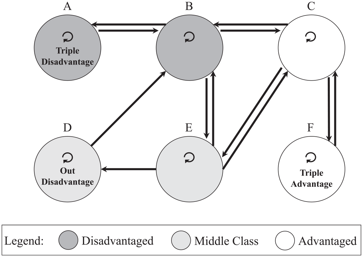
To fix our theoretical framework, Figure 1 presents an illustrative example using a neighborhood network for a city with six neighborhoods. Neighborhoods A and B are defined as disadvantaged based on the socioeconomic characteristics of their residents, and neighborhoods C and F are advantaged based on their residents. Neighborhoods D and E are middle-class. The circular directed lines represent the time residents spend within their neighborhoods—loops in network parlance—which is the phenomenon often conceptualized as (residential) neighborhood (dis)advantage in traditional neighborhood effects scholarship.

Because neighborhood A is structurally connected to only disadvantaged neighborhoods through its residents’ daily travels (to B) and visits from other neighborhoods’ (B’s) residents, A is triply disadvantaged. In an analogous way, neighborhood F is triply advantaged. Neighborhoods B and C are not doubly or triply (dis)advantaged because they are structurally connected to many different types of neighborhoods. Neighborhood D is residentially middle-class, but it is connected through its residents’ visits only to a disadvantaged neighborhood (B), so D is disadvantaged in terms of structural neighborhood linkages fostered by its residents’ travels. In a real city, residents can and will visit neighborhoods with varying frequencies, in which case ties can be weighted by the volume of flows. In addition, (dis)advantage will occur on a spectrum.

Figure 1.

Conceptual Model of Triple Neighborhood (Dis)advantage

Calculating empirical measures of triple neighborhood disadvantage requires two types of information: a measure of RND and a network of inter-neighborhood mobility within the city. We define neighborhoods as block groups, which typically comprise 600 to 3,000 people and are the lowest geographic unit at which summary statistics are publicly available. ¹ We use data on all U.S. neighborhoods from the 2011–15 American Community Survey (ACS) ² to calculate RND. Consistent with prior research (Wodtke, Harding, and Elwert 2016), we conduct a principal factor analysis of seven neighborhood characteristics: percentages of poverty, unemployment, single-headed households, public assistance receipt, adults without a high school diploma, adults with a bachelor’s degree or higher, and workers who are managers or professionals. The variables load strongly onto one factor with high reliability (Cronbach’s alpha = .85; see Part 1 of the online supplement). Nationwide, RND is a continuous variable with a mean of zero and standard deviation of .94.

Estimating a neighborhood network based on inter-neighborhood mobility within a city requires data on the home location of individuals, as well as their movements within the city. Few data sources provide the spatio-temporal coverage for a sufficiently large sample of individuals to meet this requirement, particularly for a large number of neighborhoods in multiple metropolitan areas. Fortunately, Twitter provided high-resolution data on the latitude, longitude, and time of micro-messages (tweets) sent by users opting-into Twitter’s geotagging service. ³ We selected Twitter as our application dataset, although our measures of TND are general and could be applied to other data with wide coverage and fine resolution.

Drawing on the underlying data in Wang and colleagues (2018) and Phillips and colleagues (2019), we use approximately 650 million geotagged tweets sent by 1.3 million users from October 1, 2013, to March 31, 2015, in the commuting zones surrounding the 50 most populous U.S. cities. From these data, we estimate individuals’ home locations and retain residents inside the boundaries of the 50 most populous cities. ⁴ We restrict all analyses to block groups (neighborhoods) with populations of at least 300 persons to ensure precision in our residential disadvantage measure. Similarly, we limit residents’ visits (tweets) to neighborhoods within the city boundaries that have populations of at least 300 persons.

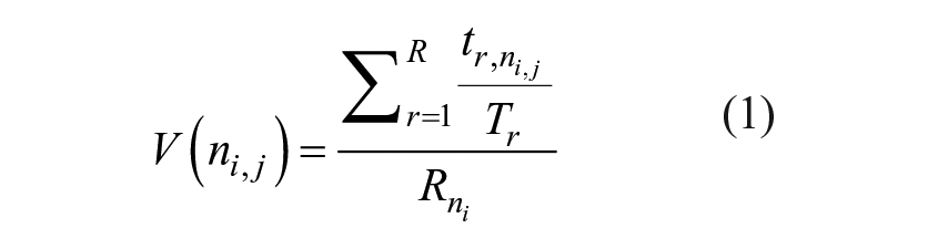
We use this subset of data to construct a valued digraph for each city comprising a set of nodes (i.e., neighborhoods), N = {n₁, n₂, . . ., n_N), a set of edges, E = {e₁, e₂, . . ., e_E}, and a set of values, V = {v₁, v₂, . . ., v_V} (Wasserman and Faust 1994). Edges denote connections between two neighborhoods, and values indicate a connection’s strength. Neighborhoods are connected when any resident (R) of neighborhood n_i visits (i.e., tweets from) another neighborhood (N). For all residents of a neighborhood, we separately calculate their fractions of visits to all neighborhoods in thecity, $\frac{t_{r,n_{i,j}}}{T_r}$ . We include tweets in their own neighborhood (i = j, or loops) to account for variation among residents in the amount of time spent in their home neighborhood. Some residents leave their neighborhoods at greater rates than other residents, and the former have a relatively larger effect on structural connections to other neighborhoods. The denominator (T_r) includes all of an individual’s tweets in the city. ⁵ We then take the mean of these fractions for all residents (r = 1, . . ., R) of the neighborhood (n_i). This generates the average fraction of visits from residents of one neighborhood to each of the city’s neighborhoods. We calculate the values of these directed connections between neighborhoods V(n_i,j) in Equation 1:

$$V\left(n_{i,j}\right)=\frac{{{\displaystyle \sum }}_{r=1}^R\frac{t_{r,n_{i,j}}}{T_r}}{R_{n_i}}$$

(1)

Note that $\forall n_i,\sum V\left(n_{i,j}\right)=1;$ thus, the difference between values for a given neighborhood (n_i) represents the relative difference in the neighborhood’s residents’ fractions of visits to all neighborhoods in the city. Aggregating all the values for a city creates the valued adjacency matrix (A) of its mobility network, where A_i,j indicates the average fraction of visits of residents from neighborhood n_i to neighborhood n_j. This includes visits within one’s neighborhood (i = i).

We use the valued adjacency matrix in Equation 2 to calculate the weighted average disadvantage level of extra-local neighborhoods to which any neighborhood (n_i) is structurally connected through its residents’ intra-city mobility patterns, which we call outdegree neighborhood disadvantage (OND):

$$ON{D}_{n_i}={\displaystyle \sum }_{j=1}^N\left(\frac{V\left(n_{i,j}\right)}{1-V\left(n_{i,i}\right)}*RN{D}_j\right),i\ne j$$

(2)

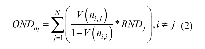
Here, RND_j represents the residential disadvantage score of the visited neighborhood. ⁶

Next, we calculate the weighted average disadvantage level of extra-local neighborhoods to which any neighborhood (n_i) is structurally connected through the intra-city visits it receives from residents of other neighborhoods, which we call indegree neighborhood disadvantage (IND). Neighborhoods vary in population size and visit rates; we adjust for these aspects in our calculations, as shown in Equation 3, where P_j is the population of a sending neighborhood (n_j):

$$IN{D}_{n_i}=\frac{{{\displaystyle \sum }}_{j=1}^{N}RN{D}_j*V\left(n_{j,i}\right)*P_j}{{{\displaystyle \sum }}_{j=1}^{N}V\left(n_{j,i}\right)*P_j},i\ne j$$

(3)

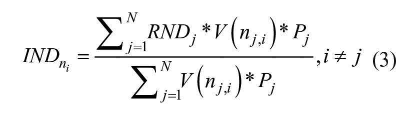
In the numerator, we weight the disadvantage of sending neighborhoods by their populations and visit shares to the neighborhood (n_i). The sum of these quantities across sending neighborhoods measures total indegree disadvantage. We divide this measure, which is not sensitive to several alternative weighting structures, by the sum of the products of the weighting variables. ⁷

We expect RND, OND, and IND to be fairly strongly correlated. Furthermore, we hypothesize that the relationship between neighborhood (dis)advantage and vitality will be strongest when multiple forms of disadvantage (RND, OND, and/or IND) compound. Thus, in addition to considering each separately, we combine them into a single measure of triple neighborhood disadvantage (TND) using principal factor analysis. RND, OND, and IND load strongly onto a single factor with high reliability (Cronbach’s alpha = .89; see also Part 1 of the online supplement).

Our OND and IND measures assume the mobility patterns observed in the geotagged tweets of Twitter users who opt to geotag are representative of the mobility patterns of the cities’ populations. This does not require Twitter users to be exactly representative of the population, nor do we expect them to be. Rather, mobility patterns estimated from their tweets must approximate actual inter-neighborhood mobility. At the municipal level, research finds that geotagged tweets reflect intermunicipal mobility patterns fairly well (Lenormand et al. 2014). Moreover, individuals’ travel distances and patterns of inter-neighborhood mobility are similar when measured by GPS, cell phone data, travel diaries, or geotagged tweets (Jones and Pebley 2014; Krivo et al. 2013; Palmer et al. 2013). A recent comparison of inter-neighborhood mobility networks in Houston, TX, calculated using geocoded tweets versus cell phone data found that the two networks correlate at .8 (see Appendix in Phillips et al. 2019). Thus, converging evidence finds mobility patterns are well approximated by geocoded tweets. ⁸

Despite the similarity of Twitter-based mobility patterns and those measured using other data, it remains possible that the existence and degree of ties between specific neighborhoods may be poorly measured by tweets. If so, then subtle differences between the actual (unobserved) mobility network and the one measured by tweets could bias our measures of IND, OND, and TND. To investigate this possibility, we re-estimate our measurers of mobility-based disadvantage in Houston, TX, using a neighborhood network constructed from cell phone geolocation data for a large number of individuals with a high level of spatio-temporal resolution. These cell phone data are not publicly available and require their own assumptions about representativeness. Yet, they are independent from our Twitter sample, and the large scale of the data and the widespread use of cell phones can mitigate some concerns about selection into the analytic sample. We find that the correlation between IND measures using the Twitter and cell-phone networks is .90, and the correlation between OND measures using the two networks is .87. Perhaps most importantly, the correlation between TND measures using the two networks is .97 (for full details, see Part 2 of the online supplement). These findings validate our assumption that inter-neighborhood mobility patterns are well approximated by geocoded tweets.

Patterns and Distribution

Table 1 presents summary statistics and correlation coefficients for the RND, IND, OND, and TND measures across all 50 cities. There is more variation in RND than in either IND or OND. This is consistent with greater socioeconomic segregation in cities’ residential patterns than in residents’ movement patterns. Residents often travel to many neighborhoods in a city (Wang et al. 2018), and in some cosmopolitan spaces residents from many different backgrounds coexist (Anderson 2011). Still, there is a high level of lived segregation as well.

Table 1.

Summary Statistics and Correlation Coefficients

	Summary Statistics		Correlation Coefficients
	Mean	SD	RND	IND	OND	TND
Residential ND	.086	1.165	1
Indegree ND	.168	.766	.804	1
Outdegree ND	−.126	.726	.757	.802	1
Triple ND	.000	.941	.914	.952	.912	1

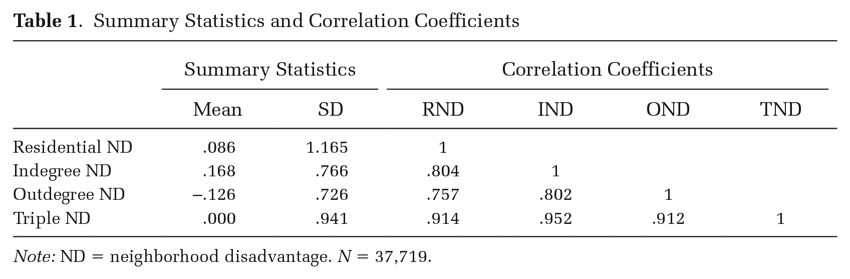
Note: ND = neighborhood disadvantage. N = 37,719.

The four measures of neighborhood disadvantage are highly correlated in neighborhoods across the 50 cities. This pattern aligns with our knowledge of structural mobility patterns within cities. Specifically, it implies that residentially disadvantaged neighborhoods are likely to see concentrated mobility-based disadvantage, and residentially advantaged neighborhoods are likely to see concentrated advantage. Despite these measures being highly correlated, the variables are not deterministic. Overall, RND explains roughly 65 and 57 percent of the variances in IND and OND, respectively, indicating the measures are separable. Across cities, there is considerable heterogeneity in these correlations. In Detroit, El Paso, and Colorado Springs, for example, the variance in IND and OND explained by RND is as low as 16 to 43 percent. As expected, the RND-TND correlation is stronger as the latter includes the former.

Figure 2 maps block groups’ RND and TND levels in Chicago, a well-studied city where the various disadvantage metrics are highly correlated. ⁹ From the Near South area to Lakeview, which includes downtown and the Loop, there is a stretch of mostly socioeconomically advantaged (low RND) neighborhoods. This is also the case in the Far Southwest Side’s Beverly and Mount Greenwood communities. By contrast, there are clusters of neighborhoods with high RND in the West Side, Southwest Side, and Far Southeast Side. Although this pattern holds for TND, some of the stark boundaries between communities blur. The abrupt change in RND values between Wicker Park and Humboldt Park is more gradual when considering mobility-based disadvantage (via TND), for example. Of course, there are still communities of mostly disadvantaged or mostly advantaged areas, and spatial (dis)advantage in Central Chicago becomes more concentrated when examining TND. Some neighborhoods near the old Cabrini-Green projects evince high levels of RND, but the levels of TND for these neighborhoods are much lower—increasing similarity with other Central City neighborhoods.

Figure 2.

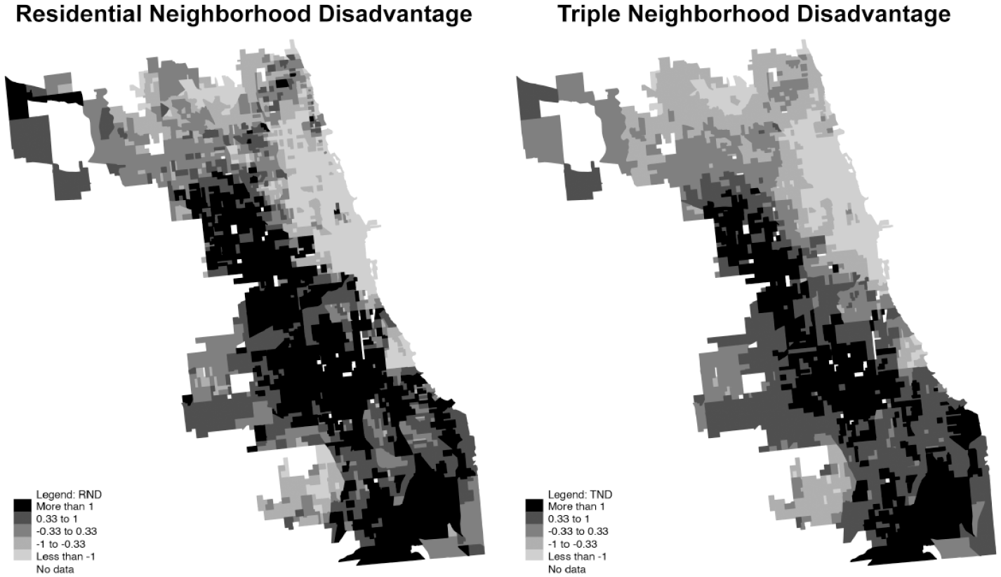
Plots of Residential ND and Triple ND in Chicago Neighborhoods

Figure 3 maps RND and TND levels in New York, where correlations between the disadvantage measures fall closer to the median of the 50-city distribution. ¹⁰ Overlap between RND and TND remains, and as with Chicago, stark boundaries between communities in RND tend to blur when examining TND. For example, Park Slope and Sunset Park in Brooklyn have a clear divide in RND, but this disparity lessens when examining TND. This is also true for the boundary between Forest Hills, especially Forest Hills Gardens, and Corona in Queens. In fact, although Brooklyn and Queens both have areas of concentrated high RND, these areas show noticeably lower levels of TND. In the Bronx, however, TND remains quite high and dense.

Figure 3.

Plots of Residential ND and Triple ND in New York Neighborhoods

Comparing TND and RND in Chicago and New York, TND reveals a spatial distribution of socioeconomic disadvantage that is at once starker in geographic concentration and yet more subtle in changes over space. In concert with our bivariate analyses, we find that RND is strongly associated with mobility-based disadvantage, although there is important variation between the metrics. This pattern reflects a model of urban mobility characterized by socioeconomic segregation. A similar pattern exists in cities with lower correlations between the disadvantage measures (see the online supplement for details on maps for all 50 cities). We now investigate how incorporating IND and OND, as well as TND, may augment or change our understanding of the role of RND in neighborhood vitality by analyzing homicide counts.

Data and Methods for Homicide Analysis

We assess triple disadvantage’s predictive power for neighborhood homicide counts in 2015 and 2016. Pooling two years of data improves precision of the estimates, as homicides can vary from year to year. Using data from 2015 and 2016 ensures RND and TND measures are largely temporally prior to the measured homicide outcomes. There is no national database of geocoded homicides, but we examine homicides using records from two sources.

First, we use data from a Washington Post investigation (Rich 2018) covering more than 52,000 homicides from 2007 to 2017 in 50 of the largest U.S. cities. ¹¹ This database defines homicides to include murder and non-negligent manslaughter; this excludes suicides, accidents, justifiable homicides, and deaths caused by negligence. Post reporters compared homicide counts to FBI records to ensure accuracy. As an independent check, we geocoded homicides from administrative records in the second and third largest cities—Los Angeles and Chicago—and found the Post counts to be highly accurate. ¹² The Post database includes the necessary homicide data for 36 cities in our analysis, comprising 9,067 homicides. ¹³ The Post reports latitude and longitude for homicides, and we used ArcGIS to tabulate block-group homicide counts based on the 2010 census boundaries from Living Atlas.

Second, we explored the municipal data portals for the 14 cities in our analysis without sufficient data from the Post database, and we located the necessary homicide data for one additional city: New York City. We use homicide data for New York neighborhoods from 2009 to 2016 reported by the New York Police Department (NYPD), assign each homicide to a street segment using the NYC Street Centerline, and spatially join homicides to block groups in ArcGIS using the TIGER shapefile. The Post database includes New York homicides for 2016 only, and comparing our 2016 NYPD data with the Post data at the neighborhood level reveals strong similarity between the two. ¹⁴

We predict neighborhood homicide counts in the 37 cities using our measures of residential and mobility-based neighborhood disadvantage, as well as a set of control variables informed by prior research. To reduce the likelihood of reverse causality explaining any association between triple disadvantage and homicide, we control for lagged homicide counts from 2009 to 2010. For example, Graif and colleagues (2019) observe that crime predicts future inter-neighborhood commuting patterns. We operationalize lagged homicide counts using a dummy variable specification with categories identifying five groups of neighborhoods: those with 0 homicides, one homicide, two homicides, three homicides, or four or more homicides from 2009 to 2010. ¹⁵

Recognizing that disadvantage in spatially proximal neighborhoods is an important predictor of neighborhood crime (Peterson and Krivo 2010), we calculate a spatial lag of RND using an unweighted average of all adjacent neighborhoods’ RND scores based on a row-normalized queen contiguity matrix. This measure helps account for the spatial clustering of disadvantage. That is, if TND predicts neighborhood homicides simply because homicides are spatially clustered and mobility-based conditions are heavily weighted toward adjacent neighborhoods, then controlling for the spatial lag of RND would substantially reduce the association between TND and homicides. On the other hand, because proximity increases the likelihood of mobility, nearby neighborhoods likely represent a key source of structural inter-neighborhood connections. Including the spatial lag of RND may then over-control and underestimate the true relationship between TND and homicides. The lagged homicide control may also exacerbate potential over-controlling bias.

Peterson and Krivo (2010) highlight city- and neighborhood-level predictors of crime. Rather than specifying city-level controls, we leverage our large sample and include city fixed effects. At the neighborhood level, we control for racial composition, home ownership composition, natural log of residential population, population density, natural log of median age, share of the population made up of young males, and residential stability. Racial composition measures are the percentages of residents that are Hispanic and non-Hispanic black. Ownership composition is the share of all homes occupied by owners. Population density is the number of residents divided by the land area in square footage, which we transform using the natural log. Young male share of the population is the percentage of residents that are males between ages 15 and 34. Residential stability is the percentage of homes occupied by the same householder since 1999, regardless of ownership status. We calculate these measures using the 2011–15 ACS.

We estimate the relationships between our focal/control variables and neighborhood homicide counts using negative binomial regression models, because the dependent variable is overdispersed counts. Equation 4 presents our model of mean homicide count:

$$ln\left({\mu }_{cn}\right)={\beta }_0+{\beta }_c{\delta }_c+{\beta }_h{d}_h+{\beta }_x{x}_{cn}$$

(4)

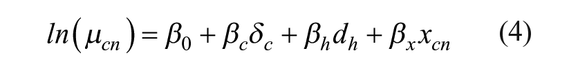
Specifically, we predict the homicide count in neighborhood n in city c with city dummy variables (δ_c), dummy variables representing lagged homicide count (d_h), and a vector of covariates (x_cn) including our measure(s) of neighborhood disadvantage and control variables. We implement Allison and Waterman’s (2002) method for fixed-effects negative binomial models ¹⁶ by using city dummies to adjust for characteristics invariant within cities. We allow the functional form of the relationships between the different neighborhood disadvantage measures and homicide count to be nonlinear by introducing quadratic and cubic terms; we select which term(s) to include using the Bayesian Information Criterion (BIC) statistic.

We estimate a sequence of models adding measures of neighborhood disadvantage to answer two questions. First, is mobility-based disadvantage independently related to homicide? Here, we consider the magnitude of the associations of IND, OND, and TND with homicides. We calculate average adjusted predicted homicide counts, conditional on fixed effects and controls, at illustrative values from the 1st to 99th percentiles of neighborhood disadvantage measures. Given the large sample size, this range does not include outliers. These average adjusted predictions provide a straightforward metric for assessing the magnitude of relationships as well as a metric that accounts for the differences in variance of the neighborhood disadvantage measures by examining a uniform 99-1 gap. Second, do these variables improve our ability to explain variance in homicides across neighborhoods beyond a measure of RND? We accomplish this by examining how McFadden’s Pseudo-R², which represents an approximate measure of overall model fit, changes with the introduction of different sets of covariates.

Mechanism Sketch

Following our models of neighborhood homicides across 37 cities, we assess potential mechanisms for the relationship between TND and neighborhood homicide counts. We restrict our mechanism models to neighborhoods in Chicago because the city provides unique publicly available data on several mechanisms that do not exist for other cities. In addition, Chicago is the focus of a substantial body of research on both crime and neighborhood effects (Sampson 2012). We test five potential mechanisms: interpersonal friction, population loss, public disorder, drug activity, and (non-fatal) gun crime. We measure these using data that are generally contemporaneous with the last years of our neighborhood disadvantage variables and temporally prior to the homicide outcomes. In this way, we ensure the time ordering of the variables is appropriate.

We measure interpersonal friction as the primary factor from a principal factor analysis of four variables: the inverse hyperbolic sines ¹⁷ (IHSs) of the 2014 rates ¹⁸ of crime reports per 1,000 neighborhood population for assaults occurring in public spaces, batteries occurring in public spaces, assaults occurring in private spaces, and batteries occurring in private spaces. All four variables load strongly onto a single factor with high reliability (Cronbach’s alpha = .89; see Part 1 of the online supplement).

We measure population loss as percentage change in population from the 2010 Census to the 2012–16 ACS. We measure public disorder as the IHSs of the 2014 rates of crime reports per 1,000 population for vandalism and prostitution, as well as the IHS of the 2014 rate of 311 calls per 1,000 population for graffiti removal. ¹⁹ The three disorder variables do not load reliably onto a single factor, and we maintain them as separate variables.

We measure drug activity as the primary factor from a principal factor analysis of the IHSs of the 2014 rates of crime reports per 1,000 neighborhood population for minor marijuana crimes ²⁰ and all other narcotics crimes. Drug arrest rates, which we expect are highly correlated with filed drug crime reports, offer a meaningful measure of the visible drug activity level in a neighborhood (Warner and Coomer 2003). Both variables load strongly onto a single factor with high reliability (Cronbach’s alpha = .88; see Part 1 of the online supplement).

Finally, we measure gun crime as the total number of 2014 non-homicide crime reports involving guns. These include robberies with guns (including attempts), sexual assaults with guns (including attempted assaults), assaults and batteries involving guns, concealed carry license violations, firearm registration violations, and legal violations in the possession, use, or sale of a firearm. We transform this variable using the IHS of the rate of gun crime reports per 1,000 neighborhood population. Results are not sensitive to removing gun crime reports for robberies and sexual assaults.

We standardize the gun crime, disorder, and population loss variables using z-scores for comparability in scale with the friction and drug activity variables. Table 2 presents summary statistics for all variables in the overall analysis and the subsample of Chicago neighborhoods in the mechanism sketch models.

Table 2.

Summary Statistics for Main Homicide Models and Mechanisms Models

	Main Models		Mechanisms Models
	Mean	SD	Mean	SD
Focal Variables
Homicides (2015–16)	.306	.745	.558	1.105
Residential ND	.123	1.177	.234	1.192
Indegree ND	.212	.762	.335	.799
Outdegree ND	−.115	.737	−.169	.813
Triple ND	.038	.945	.111	1.012
Spatial Lag ND	.120	1.024	.233	1.084
Controls
Homicides (2009–10) dummy: 0 homicides (base)	.824	.381	.744	.437
Homicides (2009–10) dummy: 1 homicide	.126	.332	.164	.370
Homicides (2009–10) dummy: 2 homicides	.034	.181	.063	.243
Homicides (2009–10) dummy: 3 homicides	.010	.101	.017	.129
Homicides (2009–10) dummy: 4+ homicides	.005	.071	.012	.111
ln(population size)	7.138	.515	7.047	.440
% black	.251	.316	.349	.409
% Hispanic	.257	.274	.260	.301
ln(population density)	9.182	1.304	9.665	.794
ln(median age)	3.572	.229	3.554	.222
% young males	.152	.073	.157	.073
% owner-occupied	.481	.282	.472	.242
% long-term householder	.307	.165	.309	.172
Mechanisms
Population change (z-score)			0	1
Population change (%)			.007	.217
Graffiti (z-score)			0	1
IHS rate of graffiti calls per 1,000 pop.			3.393	1.781
Vandalism (z-score)			0	1
IHS vandalism crimes per 1,000 pop.			2.760	.936
Prostitution (z-score)			0	1
IHS prostit. crimes per 1,000 pop.			.170	.604
Friction			0	.940
IHS assault (pub.) crimes per 1,000 pop.			1.720	1.089
IHS battery (pub.) crimes per 1,000 pop.			2.455	1.240
IHS assault (priv.) crimes per 1,000 pop.			1.081	.994
IHS battery (priv.) crimes per 1,000 pop.			2.263	1.244
Drug activity			0	.888
IHS marijuana (minor) crimes per 1,000 pop.			1.423	1.331
IHS other narcotics crimes per 1,000 pop.			1.561	1.323
Gun crime			0	1
IHS gun crimes per 1,000 pop.			1.472	1.234

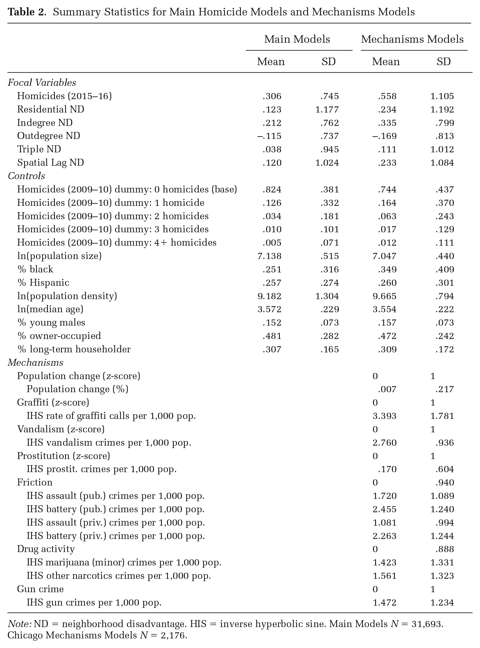
Note: ND = neighborhood disadvantage. HIS = inverse hyperbolic sine. Main Models N = 31,693. Chicago Mechanisms Models N = 2,176.

We explore potential mechanisms for the relationship between TND and homicides using mediation methods designed to analyze count outcomes (Valeri and VanderWeele 2013). This method extends the classic Baron and Kenny (1986) approach by applying a counterfactual framework and allowing modeling of treatment-mediator interactions. Omitting significant interactions can bias inferences. We estimate our outcome model using the negative binomial model in Equation 5:

$$\begin{array}{l}ln\left\{E\left(Y|A=a,M=m,C=c\right)\right\}\\ ={\theta }_0+{\theta }_{1}a+{\theta }_{2}m+{\theta }_{3}a*m+{\theta }_{c}c\end{array}$$

(5)

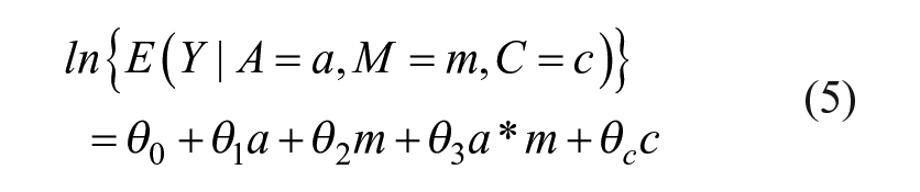
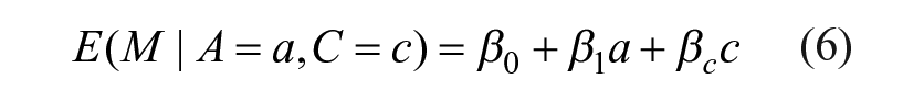
where Y is homicide count, A is treatment (TND), M is a potential mediator (mechanism), and C is a vector of controls. We fit the following linear model for the mediator:

$$E(M|A=a,C=c)={\beta }_0+{\beta }_{1}a+{\beta }_{c}c$$

(6)

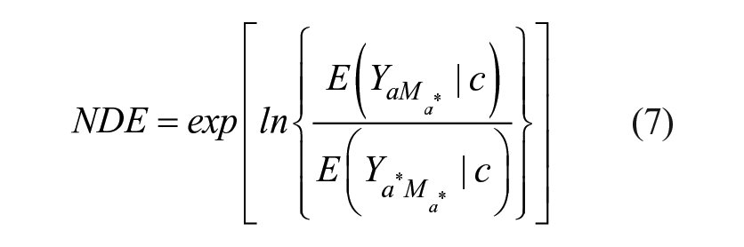
Analyzing mediation in a negative binomial outcome model requires specifying a value (a) and counterfactual (a*) for treatment to observe the difference in predicted outcome counts. We choose the 1st and 99th percentiles of TND for a and a*, respectively, to align with our pooled city analysis. Y_am, for example, represents the expected outcome when A = a and M = m.

We obtain the natural direct effect (NDE), which is on the rate ratio scale, from

$$NDE=exp\left[ln\left\{\frac{E\left(Y_{a{M}_{a^{*}}}|c\right)}{E\left(Y_{a^{*}{M}_{a^{*}}}|c\right)}\right\}\right]$$

(7)

The natural indirect effect (NIE), also on the rate ratio scale, is

$$NIE=exp\left[ln\left\{\frac{E\left(Y_{a{M}_a}|c\right)}{E\left(Y_{a{M}_{a^{*}}}|c\right)}\right\}\right]$$

(8)

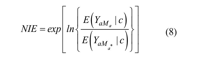
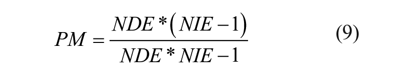
Because these are rate ratios, the total effect of a change in TND from a to a* is the product of NDE and NIE. We compute the proportion of the total effect mediated as

$$PM=\frac{NDE*\left(NIE-1\right)}{NDE*NIE-1}$$

(9)

Valeri and VanderWeele (2013) offer further details on this method. Importantly, this is not a causal mediation analysis, which requires a strict set of assumptions regarding mediator-outcome confounding, treatment-mediator confounding, and treatment-induced mediator-outcome confounding (see Wodtke and Parbst 2017). Instead, we consider these models exploratory and suggestive of potential reasons why TND relates to homicide, or a type of “mechanism sketch” (Morgan and Winship 2014:346–7).

Homicide and Triple Disadvantage

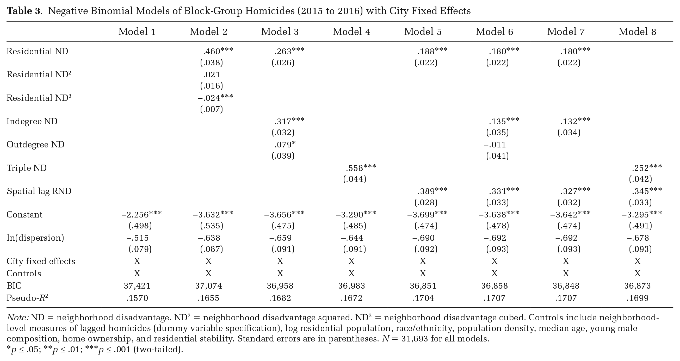
Table 3 presents results of the overall homicide models. Model 1 estimates homicide counts using all controls and city dummies, excluding any measures of neighborhood disadvantage. ²¹ The Pseudo-R² is .1570, which provides a benchmark against which we can compare Pseudo-R² changes with the addition of various measures of neighborhood disadvantage. Model 2 adds our measure of RND to Model 1. The association between RND and homicides is positive and nonlinear with a significantly stronger relationship among neighborhoods with RND scores higher than the national mean (zero). Model 2 increases the Pseudo-R² by .0085 points, which is roughly a 5 percent increase above Model 1. Table 4 presents average adjusted predicted homicide counts at the 1st and 99th percentiles of the neighborhood disadvantage variable(s). Based on Model 2, neighborhoods with very low levels of residential disadvantage have, on average, roughly .11 homicides per neighborhood from 2015 to 2016. Neighborhoods with very high levels of residential disadvantage, however, have .54 homicides, on average, during the same period. This implies a 99-1 gap of .42.

Table 3.

Negative Binomial Models of Block-Group Homicides (2015 to 2016) with City Fixed Effects

	Model 1	Model 2	Model 3	Model 4	Model 5	Model 6	Model 7	Model 8
Residential ND		.460 *** (.038)	.263 *** (.026)		.188 *** (.022)	.180 *** (.022)	.180 *** (.022)
Residential ND 2		.021(.016)
Residential ND 3		−.024 *** (.007)
Indegree ND			.317 *** (.032)			.135 *** (.035)	.132 *** (.034)
Outdegree ND			.079 * (.039)			−.011(.041)
Triple ND				.558 *** (.044)				.252 *** (.042)
Spatial lag RND					.389 *** (.028)	.331 *** (.033)	.327 *** (.032)	.345 *** (.033)
Constant	−2.256 *** (.498)	−3.632 *** (.535)	−3.656 *** (.475)	−3.290 *** (.485)	−3.699 *** (.474)	−3.638 *** (.478)	−3.642 *** (.474)	−3.295 *** (.491)
ln(dispersion)	−.515(.079)	−.638(.087)	−.659(.091)	−.644(.091)	−.690(.092)	−.692(.093)	−.692(.093)	−.678(.093)
City fixed effects	X	X	X	X	X	X	X	X
Controls	X	X	X	X	X	X	X	X
BIC	37,421	37,074	36,958	36,983	36,851	36,858	36,848	36,873
Pseudo-R2	.1570	.1655	.1682	.1672	.1704	.1707	.1707	.1699

Note: ND = neighborhood disadvantage. ND ² = neighborhood disadvantage squared. ND ³ = neighborhood disadvantage cubed. Controls include neighborhood-level measures of lagged homicides (dummy variable specification), log residential population, race/ethnicity, population density, median age, young male composition, home ownership, and residential stability. Standard errors are in parentheses. N = 31,693 for all models.

*

p ≤ .05; ^**p ≤ .01; ^*** p ≤ .001 (two-tailed).

Table 4.

Average Adjusted Predicted Homicide Count Based on Models in Table 3

	Model 1	Model 2	Model 3	Model 4	Model 5	Model 6	Model 7	Model 8
Residential ND:
1st percentile (–2.1)		.11(.02)	.14(.01)		.18(.01)	.18(.01)	.18(.01)
99th percentile (2.5)		.54(.04)	.47(.02)		.42(.01)	.41(.01)	.41(.01)
Indegree ND:
1st percentile (–1.4)			.16(.01)			.23(.02)	.23(.02)
99th percentile (1.8)			.44(.02)			.36(.01)	.36(.01)
Outdegree ND:
1st percentile (–1.6)			.26(.02)			.32(.03)
99th percentile (1.6)			.34(.02)			.30(.01)
Triple ND:
1st percentile (–1.8)				.08(.01)				.17(.02)
99th percentile (2.0)				.69(.05)				.43(.02)
Spatial Lag ND:
1st percentile (–1.9)					.11(.01)	.13(.01)	.13(.01)	.12(.01)
99th percentile (2.1)					.53(.02)	.48(.02)	.48(.02)	.49(.02)
Predicted 95-5 Gaps
Residential ND		.42	.33		.24	.23	.23
Indegree ND			.28			.13	.12
Outdegree ND			.08			−.01
Triple ND				.61				.27
Spatial lag ND					.42	.35	.35	.37

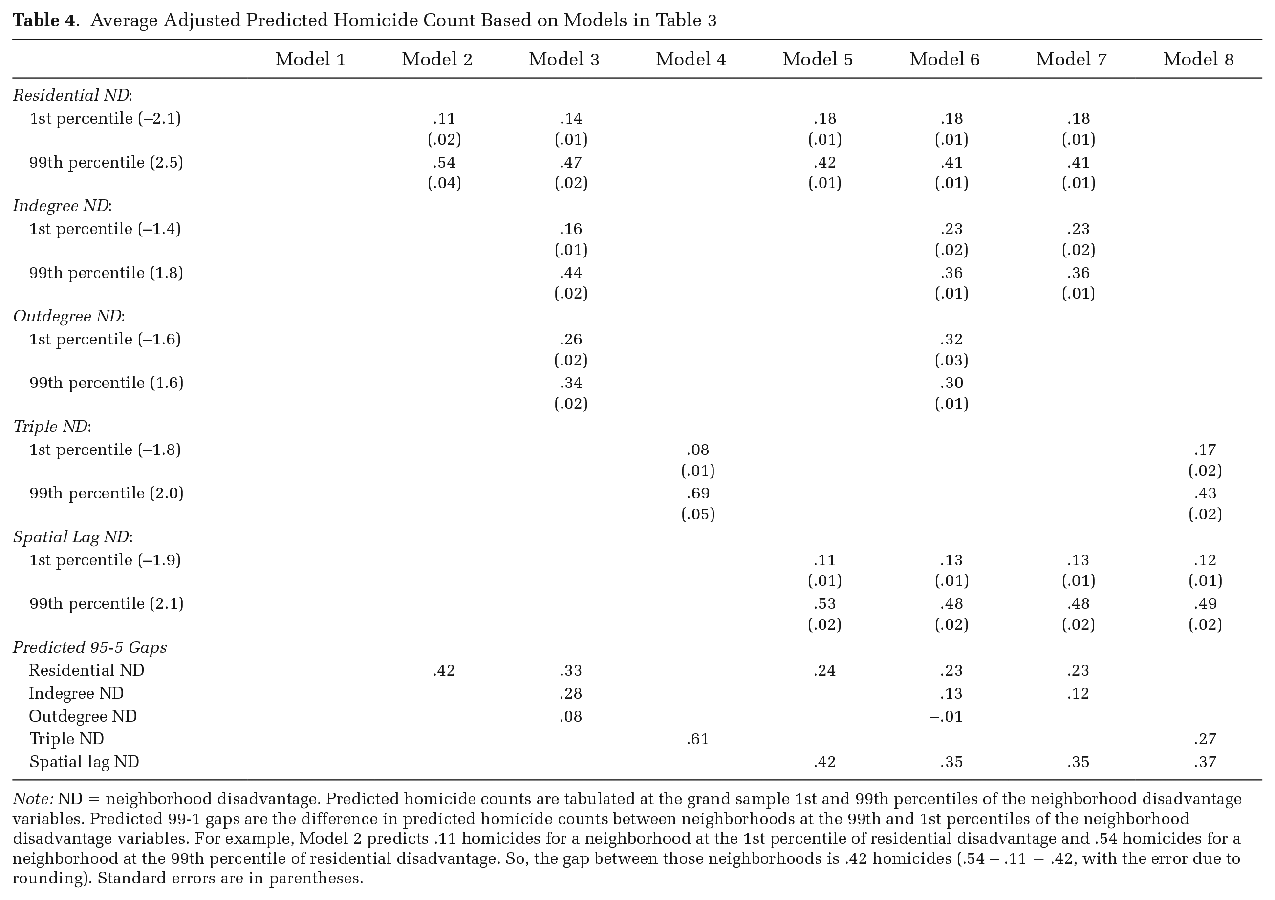
Note: ND = neighborhood disadvantage. Predicted homicide counts are tabulated at the grand sample 1st and 99th percentiles of the neighborhood disadvantage variables. Predicted 99-1 gaps are the difference in predicted homicide counts between neighborhoods at the 99th and 1st percentiles of the neighborhood disadvantage variables. For example, Model 2 predicts .11 homicides for a neighborhood at the 1st percentile of residential disadvantage and .54 homicides for a neighborhood at the 99th percentile of residential disadvantage. So, the gap between those neighborhoods is .42 homicides (.54 – .11 = .42, with the error due to rounding). Standard errors are in parentheses.

Model 3 adds IND and OND to Model 2. Both have significant positive associations with homicide count, although the IND–homicide association is nearly four times as strong. The 99-1 homicide gap by IND is .28, and the 99-1 gap by OND is .08. Adding IND and OND increases the Pseudo-R² from Model 2 by .0027 points—or roughly one-third of the increase in Pseudo-R² from adding RND to Model 1. In addition, the reduction in the BIC suggests Model 3 is a better overall model than Model 2. Adding IND and OND also attenuates the observed association between RND and homicides. The 99-1 homicide gap based on RND declines significantly from .42 based on Model 2 to .33 based on Model 3—a reduction of 21 percent. Moreover, the 99-1 homicide gap by RND is similar in magnitude to that by IND. This indicates that mobility-based disadvantage is an independent predictor of neighborhood homicides, and these conditions account for a nontrivial portion of the association between RND and homicides.

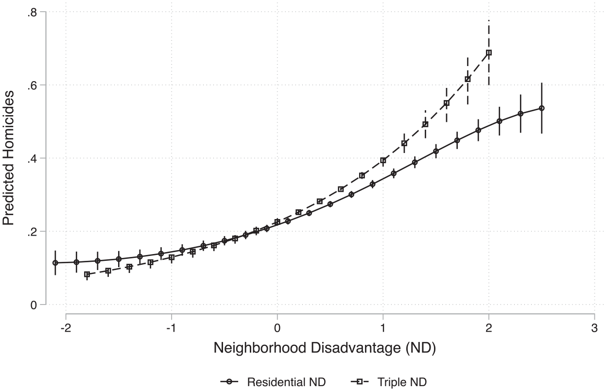
Model 4 adds our measure of TND, which incorporates RND, IND, and OND to Model 1. TND is positively and strongly associated with neighborhood homicides. Although the Pseudo-R² and BIC indicate that the parsimonious Model 4 performs slightly less well than Model 3, it nevertheless represents an improvement over a model that only considers RND and controls (Model 2). For comparison, we plot the average adjusted predicted homicide count from the 1st to 99th percentiles of RND (Model 2) and TND (Model 4) in Figure 4. Neighborhoods with very low levels of TND have significantly lower predicted homicide counts than do those with very low scores for RND. Similarly, neighborhoods with very high TND values have significantly higher predicted homicides than do those with very high scores for RND. The 99-1 homicide gap based on triple disadvantage (.61) is over 45 percent larger than the 99-1 gap based on residential disadvantage (.42).

Figure 4.

Average Adjusted Predicted Homicide Count: Residential Neighborhood Disadvantage (Table 3, Model 2) versus Triple Neighborhood Disadvantage (Table 3, Model 4)

Model 5 assesses how the association between RND and homicides changes with the introduction of the spatial lag of RND. Essentially, this model examines the role of the residential and immediately adjacent neighborhoods’ socioeconomic context. RND remains positively associated with homicides, but as was the case when adjusting for mobility-based disadvantage, this association attenuates significantly when controlling for the spatial lag of RND. The 99-1 gap in homicide count by the spatial lag of RND is nearly double the gap by RND itself. This suggests disadvantage levels of adjacent neighborhoods are more predictive of a neighborhood’s homicide count than is a neighborhood’s own levels of disadvantage.

Model 6 adds both measures of mobility-based disadvantage and the spatial lag of RND to Model 2. IND is positively associated with homicides, but controlling for spatial lag RND reduces the association between OND and homicide counts to essentially none. Model 7 removes the OND variable from Model 6, and this model provides the best overall fit of the data. This suggests a model of homicide counts including RND and its spatial lag is missing important explanatory power gained by accounting for mobility-based disadvantage. RND, its spatial lag, and IND are all associated with significant increases in a neighborhood’s homicide count.

Finally, Model 8 predicts homicide counts by TND, spatial lag RND, controls, and city fixed effects. Both TND and the spatial lag have significant positive associations with homicides. The 99-1 gap in average adjusted predicted homicides is moderately larger for the spatial lag of RND than for TND, but TND remains a substantively important predictor. Figure 5 plots average adjusted predicted homicides by TND and the spatial lag of RND based on the estimates in Model 8. The association between TND and homicides is much more linear in nature, and the divergence in the slope of predicted homicides by TND versus the spatial lag of RND emerges among neighborhoods that have moderate to high levels of disadvantage.

Figure 5.

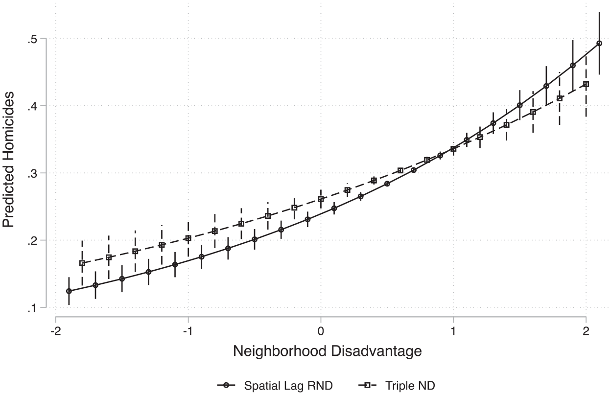
Average Adjusted Predicted Homicide Count by Triple Neighborhood Disadvantage and the Spatial Lag of RND (Table 3, Model 7)

To test the consistency of our results in two well-studied cities with distinct urban forms, we replicate our models separately for Chicago and Los Angeles (see Part 4 of the online supplement). In both cities, the pattern of results is similar to our pooled analysis. Although the standard errors are larger with the single-city sample, in both cases we find a greater 99-1 homicide gap by TND than RND. In Chicago, the preferred model (based on the BIC) includes terms for TND and the spatial lag of RND; in Los Angeles, the preferred model includes only TND. The consistency of our findings regarding TND suggests its significance is not an aberration of a rare city type.

Potential Mechanisms

We now assess how five potential mechanisms—population change, disorder, drug activity, interpersonal friction, and gun crime—potentially explain the observed relationship between TND and homicide count in Chicago. As shown in Table 2, there is just over one homicide per every two neighborhoods in Chicago between 2015 and 2016, which is roughly 60 percent higher than in the 37-city sample. RND, IND, and TND also tend to be slightly higher in Chicago neighborhoods, whereas OND is slightly lower in Chicago.

For Chicago, our preferred model without mechanisms includes a measure of TND plus controls (see Table S7 in the online supplement). We exclude the spatial lag of RND to avoid over-controlling, which would downwardly bias the TND–homicide relationship for which we explore mediation. In Chicago, TND has a strong, positive relationship with homicide count. A neighborhood at the 1st percentile of Chicago TND is predicted to experience .13 homicides from 2015 to 2016. A neighborhood at the 99th percentile of TND is predicted to experience one homicide during that time—more than seven times as much as the neighborhood at the 1st percentile.

Table 5 presents results of the mediation models. We suppress coefficients for controls in the outcome and mediator models for brevity (for full results, see Part 3 of the online supplement). Model 1 tests population change as a potential mechanism for the TND–homicide relationship. In the outcome model, both are significantly associated with homicide count in the expected direction, and in the mediator model, TND is negatively associated with population change. Furthermore, population change mediates 12 percent of the 99-1 homicide gap by TND. We view this as evidence that population change is at most a weak mechanism for the TND–homicide relationship given the lack of controls for other potential mechanisms in this model. ²²

Table 5.

Mediation Models of the Relationship between Triple Neighborhood Disadvantage and Chicago Block-Group Homicides

	Model 1	Model 2	Model 3	Model 4	Model 5	Model 6	Model 7
Mediator	Pop. Change	Vandalism	Graffiti	Prostitution	Drugs	Friction	Gun Crime
Homicide Model (Negative Binomial), Select Parameter Estimates
Triple ND (TND)	.507 *** (.083)	.615 *** (.096)	.526 *** (.083)	.545 *** (.083)	.446 *** (.096)	.571 *** (.101)	.584 *** (.098)
TND × Mediator	.001(.052)	−.218 ** (.069)	−.156 ** (.055)	−.102 * (.042)	−.192 ** (.062)	−.267 *** (.071)	−.193 ** (.065)
Pop. change	−.180 ** (.066)
Vandalism		.567 *** (.080)
Graffiti			.347 *** (.068)
Prostitution				.172 ** (.054)
Drugs					.655 *** (.079)
Friction						.783 *** (.092)
Gun crime							.655 *** (.085)
Mediator Model (OLS), Select Parameter Estimate
Triple ND	−.163 *** (.042)	.184 *** (.036)	−.040(.036)	.138 ** (.047)	.400 *** (.026)	.309 *** (.026)	.215 *** (.027)
Total Effect (TE), Natural Direct Effect (NDE), and Natural Indirect Effect (NIE) of an Increase in Triple Neighborhood Disadvantage from −1.9 to 1.9 on Homicides (estimates on the rate ratio scale)
TE	7.672 *** (.084)	12.086 *** (.129)	6.261 *** (.095)	8.210 *** (.085)	13.261 *** (.120)	18.161 *** (.150)	13.784 *** (.120)
NDE	6.872 *** (.085)	10.855 *** (.134)	6.309 *** (.095)	8.305 *** (.086)	8.529 *** (.136)	13.153 *** (.163)	10.892 *** (.127)
NIE	1.116 *** (.013)	1.113 *** (.021)	.992 * (.004)	.988 * (.006)	1.555 *** (.036)	1.381 *** (.035)	1.265 *** (.023)
% Mediated	12.0%	11.1%	−1.0%	−1.4%	38.6%	29.2%	22.6%

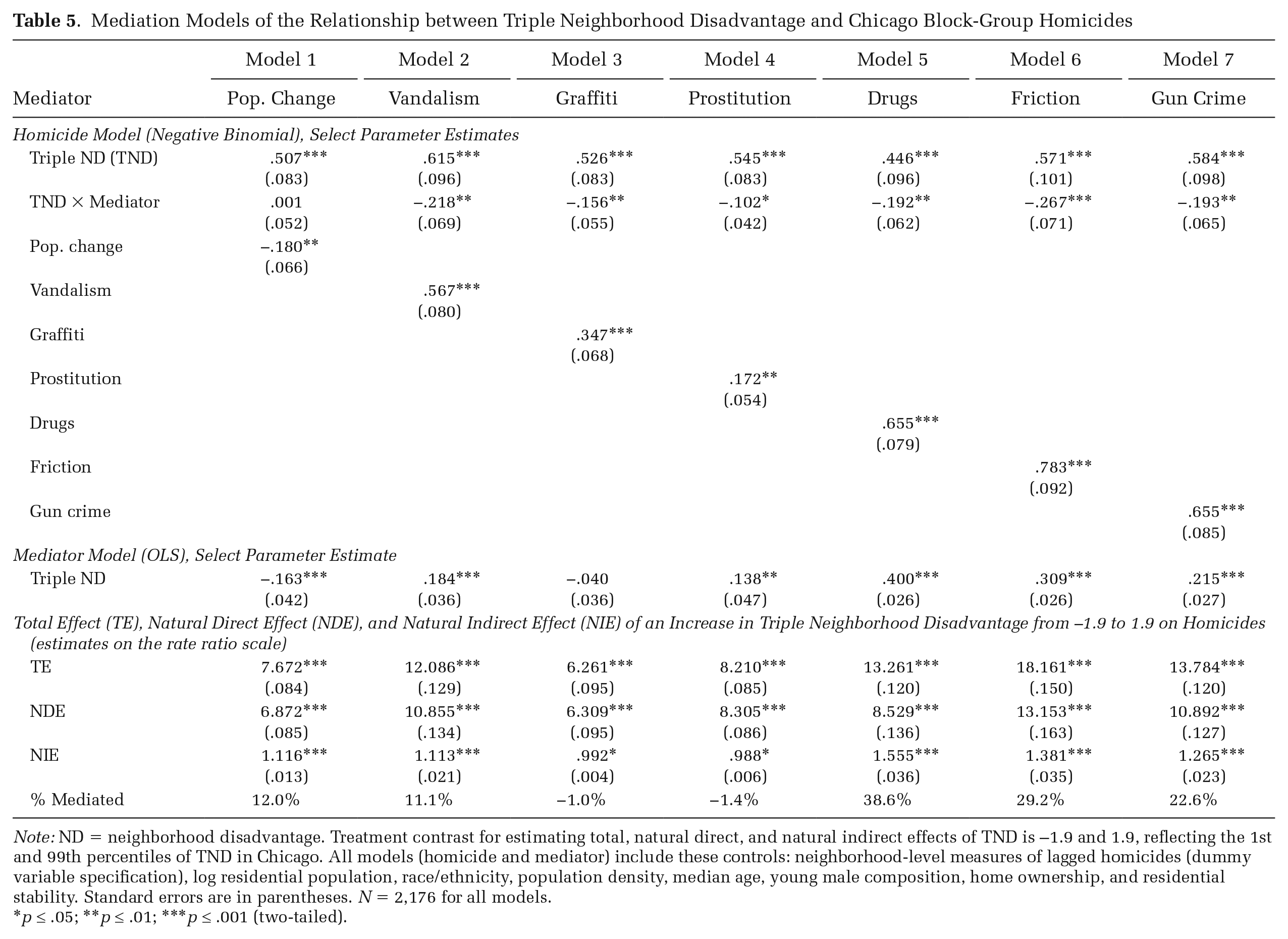
Note: ND = neighborhood disadvantage. Treatment contrast for estimating total, natural direct, and natural indirect effects of TND is −1.9 and 1.9, reflecting the 1st and 99th percentiles of TND in Chicago. All models (homicide and mediator) include these controls: neighborhood-level measures of lagged homicides (dummy variable specification), log residential population, race/ethnicity, population density, median age, young male composition, home ownership, and residential stability. Standard errors are in parentheses. N = 2,176 for all models.

*

p ≤ .05; ^**p ≤ .01; ^***p ≤ .001 (two-tailed).

Model 2 tests vandalism—the first of our three measures of disorder—as a potential mechanism. Vandalism and TND are both significantly positively associated with homicides. In addition, the coefficient on their interaction is significant and negative. This indicates that reductions in homicides associated with lower levels of TND and vandalism are particularly strong in neighborhoods at the low end of their distributions, whereas the strength of increases in homicides associated with higher levels of TND and vandalism attenuates at the high end of their distributions. As a result of this significant interaction, which we find to varying degrees for the remainder of the mechanisms as well, the estimated 99-1 homicide gap by TND is relatively large compared to Model 1. In assessing vandalism as a potential mechanism for the TND–homicide relationship, however, we find that vandalism is at most a weak mechanism as it mediates only 11 percent of the TND–homicide relationship in Model 2.

Models 3 and 4 test our other two measures of disorder: graffiti and prostitution. Neither mediates any of the relationship between TND and homicide. In Model 3, the association between TND and graffiti is essentially null. In Model 4, the associations of prostitution with both TND and homicide are quite modest; when coupled with the negative interaction between prostitution and TND on homicide, this leads to the negligible, negative net indirect effect.

Model 5 tests drug activity as a mechanism for the TND–homicide relationship. There is a moderately strong, positive association between TND and drug activity, and both variables have strong, positive associations with neighborhood homicides. In this model, drug activity mediates nearly two-fifths of the 99-1 homicide gap by TND. This suggests drug activity is a plausible mechanism for a moderate portion of the TND–homicide relationship.

Models 6 and 7 test interpersonal friction and gun crime as mechanisms. Both variables are moderately associated with TND and strongly associated with homicide. In Model 6, interpersonal friction mediates 29 percent of the especially large 99-1 homicide gap by TND. In Model 7, the 99-1 homicide gap by TND is less strong but still pronounced, and gun crime can mediate roughly 23 percent of the gap. In summary, of the mechanisms tested, drug activity, friction, and gun crime appear most salient. Each explains a moderately large portion of the 99-1 homicide gap by TND in Chicago neighborhoods.

We also replicated the mediation models in Table 5 replacing TND with, separately, measures of RND, IND, and OND. For each component, the primary mediators remained the same and with the same rank in terms of percent mediated as in the TND models in Table 5. For RND, drug activity was relatively more important, whereas for IND friction increased in relative importance—nearly equaling drug activity in percent mediated. This pattern of results aligns with our theoretical expectations about mobility-based disadvantage and disputatious encounters.

As a final assessment of the added value of our mobility-based approach to neighborhood (dis)advantage, we estimated ordinary least squares (OLS) models of the three key mediators. Predicting neighborhood-level variation in each using RND, IND, and OND along with all controls, we find that the standardized coefficient for IND is always larger than that for RND. In fact, for friction, the IND coefficient is 85 percent larger than the RND coefficient, and for gun crime the IND coefficient is 130 percent larger. ²³ Controlling for IND and RND, the OND coefficient is negligible and not significant. These additional findings further confirm the influence of IND in neighborhood crime levels.

Robustness and Validity Checks

We test the robustness of our main models to three alternative specifications (see Part 5 of the online supplement). Our main models use fixed-effects negative binomial regressions (Allison and Waterman 2002) to estimate the relationship between triple neighborhood disadvantage and homicide counts. Although results indicate significant overdispersion, we also estimate a fixed-effects Poisson model and find substantively similar results. We further consider the potential for outsized influence of New York City (n = 5,934) on our results. Re-estimating our main models while excluding New York yields substantively similar results. Finally, we re-estimate our main models without the lagged homicide dummies; predictably, the associations of neighborhood disadvantage variables with homicides strengthen, although the pattern of findings is consistent.

In addition to proper model specification, our estimates rely on the validity of inter-neighborhood mobility patterns observed with geocoded tweets. We earlier described several validity checks on the Twitter data, including the strong correlations of our estimated neighborhood network and values of TND for Houston with those estimated using cell phone GPS. One additional concern might be that mobility patterns in neighborhoods with few Twitter users are subject to measurement error due to small sample bias. To evaluate this, we re-estimate the correlation coefficients for IND and OND with RND, neighborhood poverty, and neighborhood racial demographics while stratifying the sample by the number of home Twitter accounts observed in the neighborhood (see Part 6 of the online supplement). The latter measures are based on census data with high precision. Thus, the extent to which correlations for IND and OND are similar between neighborhoods with few home accounts and those with a larger number of home accounts improves our confidence in the measures of mobility-based disadvantage. Among the neighborhoods with fewer than five home Twitter accounts, correlations for IND and OND with key neighborhood demographics remain quite strong and substantively similar to both the full sample and the sample of neighborhoods with five or more home Twitter accounts.

We also re-estimate our main homicide models stratifying the sample by whether the neighborhood has at least five home Twitter accounts (see Part 7 of the online supplement). The results for both subsamples are quite similar to those for the full sample, but the similarity is especially strong for the subsample of neighborhoods with five or more accounts. The pattern of results suggests that including neighborhoods with fewer accounts may conservatively bias estimated relationships between mobility-based disadvantage and homicide. We then re-estimate our main models weighting neighborhoods by the natural log of number of home Twitter accounts. These results are again similar to our main models. This increases our confidence in our measurement of mobility-based disadvantage—even for neighborhoods with fewer Twitter accounts.

Next, we consider whether variation in ambient population could explain part of our findings (see Boivin and Felson 2018; Hipp et al. 2019). If higher shares of visits from low-income neighborhoods are associated with more visits from all neighborhoods, then a positive relationship between IND and homicide may reflect increased opportunity for homicide due to larger ambient populations. We measure ambient population as the natural log of block-group indegree weighted by sending neighborhood population. Across all neighborhoods, the correlation between IND and ambient population is –.14. This suggests highly visited locations are less likely to be visited by residents of economically-disadvantaged neighborhoods. We also re-estimate our main models by adding this control for ambient population. The results are highly similar, in fact with a slightly stronger association between TND and homicide count (see Part 8 of the online supplement). ²⁴ Thus, ambient population is neither confounding nor does it explain the TND–homicide relationship.

Another threat to validity is spatial autocorrelation of errors biasing significance tests. To address this, we estimate a sequence of spatial error models for both Chicago and Los Angeles. ²⁵ The pattern of results (see Part 9 of the online supplement) is quite similar to the main models for Chicago and Los Angeles (Part 4 of the online supplement). In both cities, the model most likely to explain the observed pattern of homicides, based on the BIC statistic, includes TND as a covariate. The significant relationship between TND and homicides also persists when controlling for spatial lag RND.

Conclusions

Summary of the Argument and Results

The concept of triple neighborhood disadvantage (TND) builds on the idea that the resources and well-being of a neighborhood are not simply a function of its residents’ socioeconomic characteristics, or those of adjacent neighborhoods. Rather, residents’ everyday mobility patterns generate connections between neighborhoods throughout the metropolis that create mobility-based (dis)advantage correlated with, but distinct from, residential and spatially proximal neighborhood conditions.

This idea aligns with the higher-order structure of social stratification in cities (Sampson 2012: Part IV). Research on neighborhood effects often faces criticism for ignoring such higher-order effects; here, we link micro-level block groups with city-level structural mobility patterns to uncover one way that neighborhood resources and intercity mobility patterns work together to reinforce spatial inequality. Structural mobility patterns provide an important source of (dis)advantage for neighborhoods, a resource that is largely unmeasured—primarily due to data limitations—in prior research on neighborhood effects.

Analyzing neighborhood-level homicides as a key measure of neighborhood well-being for 37 U.S. cities, we find that TND adds explanatory power both in terms of homicides themselves and in explaining the relationship between residential neighborhood disadvantage (RND) and homicides. A long body of research highlights RND as an important predictor of neighborhood violent crime (e.g., Peterson and Krivo 2010; Sampson 2012). Yet, mobility-based disadvantage can explain roughly one-fifth of the relationship between RND and homicide counts. Moreover, when compared to adding only RND to a baseline model of homicide counts using controls, including indegree neighborhood disadvantage (IND), outdegree neighborhood disadvantage (OND), and RND improves the explanatory power appreciably—by 32 percent more than adding only RND on McFadden’s Pseudo-R². For homicides, IND appears to be more influential than OND. Whether this holds for other types of crime or forms of neighborhood vitality is worth future exploration. Focusing on Chicago neighborhoods, we find that drug activity, interpersonal friction, and gun crime are potential mechanisms for the relationship between TND and homicides.

These findings suggest traditional models of homicide and crime omit an important source of inter-neighborhood variation: disadvantage in the neighborhood network. The salience of TND in our results aligns with recent research showing neighborhood linkages formed by residents’ co-offending facilitate the spread of homicide (Papachristos and Bastomski 2018). Indeed, these connections in crime may be occurring because neighborhoods are similarly experiencing TND. Triple disadvantage likely increases the interactions between similar status individuals, which heightens the risk for conflict (Anderson 1990, 1999; Gould 2003), and we find interpersonal friction to be a plausible mechanism for the TND–homicide association. Still, we expect this relationship is more than just a compositional effect of individuals and instead reflects the differential abilities of neighborhoods to form coalitions to access public crime-prevention resources.

Limitations and Suggestions for Future Research

We acknowledge several limitations of our analysis that deserve further consideration. First, our models of neighborhood homicides do not implement a formal causal identification strategy. We do find a substantive and statistically significant relationship between TND and homicides adjusting for city-level fixed effects, lagged homicides, and a set of theoretically informed covariates measured with precision. Nevertheless, no observational study can fully discount omitted variable bias. Future research leveraging natural experiments that change the nature of inter-neighborhood mobility might provide a stronger causal design.

Second, although our estimates based on geocoded tweets are high-quality in terms of available data at large scale and align well with other estimates of mobility patterns using alternative data (Phillips et al. 2019; see also Part 2 of the online supplement), they lack the comparatively high precision of census-based measures of RND. These differences in reliability may bias estimates of the effect of mobility-based disadvantage. For example, our finding of a substantively strong association between such disadvantage and neighborhood homicide counts while controlling for the comparatively precise measures of RND and its spatial lag suggests TND plays an important role in urban neighborhood conditions. In the future, if mobility data are publicly available from smartphones or fitness trackers consistently used by many individuals, these could provide added value. This would be especially true if data exist for a representative sample of people in a large number of neighborhoods. At present, our validation test in Houston demonstrates that Twitter data offer a good approximation of recent mobility patterns.

A third potential limitation is that our mechanism sketch, which is also not meant to identify a causal effect, is incomplete. Any one mechanism accounts for at most 39 percent of the relationship between TND and homicides in Chicago. We include several theoretically relevant mechanisms measured with high-quality data. Yet, by design, the mechanisms arise mainly from the criminology tradition and reflect a pathway model from TND to criminogenic conditions and situations—especially those that increase or involve disputatious encounters—to homicide itself. Neighborhood resilience, collective efficacy, and political power represent theoretically distinct, although plausible, mechanisms for the relationship between TND and homicides that we were unable to test.

Implications for Neighborhood Inequality Studies

Despite these limitations, and allowing for measurement error, we have shown that the concept of triple disadvantage can be reliably measured and that it has independent explanatory power, a proof of concept that can be expanded in future research. Moreover, the theoretical underpinnings are general in nature and not limited to violence. Research examining the relationship between TND and neighborhood capacity or collective efficacy, for example, is worthwhile on its own and not just as a mechanism for explaining crime. Triply disadvantaged neighborhoods may lack the necessary coalitions to achieve significant public or private investment, as well as the social or spatial proximity to critical organizational resources (Marwell and Morrissey 2020; Molotch 1976).

In addition to its role in shaping dimensions of neighborhood capacity, TND may be a leading indicator of gentrification. Recent decades have seen a clear rise in gentrification among urban neighborhoods (Ellen and O’Regan 2008; Hyra 2012), and this has been met with increased scholarly interest (for a recent review, see Brown-Saracino 2017). Our maps of RND and TND reveal lower levels of TND than RND among gentrifying neighborhoods. For example, in New York City, we find modest levels of TND in the high-RND neighborhoods of Brooklyn and Queens that experienced gentrification in the past 10 years. This result may help explain the negative association between gentrification and homicide (Papachristos et al. 2011). Given its potential role in neighborhood capacity and gentrification, we believe TND is likely to be an important measure in understanding the structure of a city.

Implications for Studies of Epidemics and Diffusion

Neighborhood networks and TND have several implications for the COVID-19 crisis and pandemics generally. First, mobility networks offer a pathway for community spread (Phillips et al. 2019), although the role of TND in spread is less clear. Triply disadvantaged neighborhoods receive fewer visitors on average, which may be protective. Still, residents of triply disadvantaged neighborhoods may travel further to access essential goods or services, be overrepresented among those required to work in person, or have other COVID risk factors, eroding the benefits of relative isolation. In terms of general neighborhood vitality, a pandemic could be equalizing if mobility declines and structural neighborhood ties erode or become less salient.

Yet, the opposite might be true. Triply advantaged neighborhoods may effectively preserve community capacity and secure scarce but critical resources. Specific to our analysis, we do not have a clear expectation for neighborhood-level inequality in crime by TND during a pandemic. To the extent that crime declines due to reductions in mobility limiting opportunities, disparities may lessen. Nevertheless, in strained cities, triply disadvantaged neighborhoods may find it particularly difficult to access institutional resources and social investments that limit crime. These topics merit future research.

Implications for Racial and Ethnic Inequality Studies

We also expect TND to have important implications for known racial and ethnic disparities in neighborhood resources (Charles 2003; Massey and Denton 1993). The strong correlation between RND and TND suggests non-white neighborhoods are much more likely to be triply disadvantaged. In fact, TND is more unequally distributed than RND. Within our 50-city sample, mostly black and mostly Hispanic neighborhoods are 31 and 41 times as likely as mostly white neighborhoods to have RND scores at least one standard deviation above the national mean. ²⁶ Yet, mostly black and Hispanic neighborhoods are 77 and 84 times as likely as mostly white neighborhoods to have TND scores at least one standard deviation above the mean. This pattern suggests indicators focused solely on RND obscure the magnitude of disparities, and long-standing racial inequality in neighborhood socioeconomic conditions (Sharkey 2014) extends to segregation in urban mobility patterns with even greater force. Racial disparities also compound across measures of RND, IND, and OND. Almost no white neighborhoods are triply disadvantaged, and essentially no black or Hispanic neighborhoods are triply advantaged.

In summary, our results show that mobility-based disadvantage is an understudied and important component of inequality, one that may take on growing significance. Neighborhood socioeconomic segregation is at historic levels and increasing (Reardon et al. 2018). Preferences for social homophily are well-established (McPherson, Smith-Lovin, and Cook 2001). These dynamics reinforce the segregated inter-neighborhood mobility networks that give rise to triple neighborhood (dis)advantage, which is poised to play an increasingly prominent role in maintaining and exacerbating inequality in the United States.

Supplemental Material

sj-pdf-1-asr-10.1177_0003122420972323 – Supplemental material for Triple Disadvantage: Neighborhood Networks of Everyday Urban Mobility and Violence in U.S. Cities

Supplemental material, sj-pdf-1-asr-10.1177_0003122420972323 for Triple Disadvantage: Neighborhood Networks of Everyday Urban Mobility and Violence in U.S. Cities by Brian L. Levy, Nolan E. Phillips and Robert J. Sampson in American Sociological Review