Sage Journals: Discover world-class research

Abstract

Policymaking that aims to protect families and foster economic growth ought to be informed by a clear understanding of how employment, benefits, and family well-being interact. Here, we conduct a broad assessment of employment trends among low-income Americans, showing that, in recent decades, people with low income have become more highly educated and less likely to be married, and the share that is Hispanic has increased. We also find that these shifting characteristics do little to explain change in employment over time. Our findings also contribute to a growing literature that documents how social benefits for nonelderly adults increasingly reward and encourage work: benefits have become more generous to low-income adults with children who have substantial earnings, while they have remained relatively stable for childless adults. Low-income families with children and substantial earnings received more income from social benefits in the past decade than they did 30 years ago.

Keywords

employment labor supply low-income workers social benefits maternal employment Earned Income Tax Credit

Understanding ways in which employment, social benefits, and family well-being interact is key to designing better policies both to protect families and to foster economic growth. Fluctuations in the unemployment rate affect the shares of people living in poverty, rates of food insecurity, and other measures of well-being (Bitler and Hoynes 2015; Hoynes 2000). The impacts of economic cycles are larger for vulnerable populations such as low-income families, families with Black or Hispanic members, and families with children. Of course, longer-run trends in employment patterns and wages—which are influenced by changes in automation, trade patterns, and other factors—also play a key role in family well-being and the design of social benefits programs.

Many workers in low-income families are employed in jobs that are unstable and offer limited wage growth and other benefits (Acs and Nichols 2007; Butcher and Schanzenbach 2018; Kim 2000). Evidence is mixed on the extent to which low-wage workers in low-income families are able to move up the job ladder, with some studies finding essentially no improvement over time (Gabe, Abel, and Florida 2018; Looney and Manoli 2016) and others finding modest but positive gains (Kuka and Shenhav 2024; Neumark, Asquith, and Bass 2020). Either way, many workers in low-income families rely on significant support from the social safety net to help support themselves and their families.

Over the past three decades, social benefits policies have dramatically shifted in terms of their orientation toward work. In the 1990s, the addition of strict time limits and other reforms to the cash welfare program combined with expansion of the Earned Income Tax Credit (EITC), which provided incentives and benefits for employment to low-income parents, fundamentally changed the employment landscape among this population (Bahk, Moffitt, and Smeeding, this volume; Blank 2002). Subsequent changes in both health insurance coverage, due to the Affordable Care Act (Dillender, Heinrich, and Houseman 2022), and in SNAP (Supplemental Nutrition Assistance Program) work requirements (Cook and East 2024) may have also had an impact on the patterns of employment among low-income families. Finally, although the evidence is mixed, state and local increases in minimum wages may have also altered the landscape for low-income workers, specifically affecting employment and other measures of well-being (Cengiz et al. 2019; Clemens and Strain 2021; Jardim et al. 2022).

In this article, we begin by documenting broad declines in employment over time (see also Abraham and Kearney 2020). Next, we describe who is included in the low-income population and how their average family compositions, educational attainment, race and ethnicity, and other characteristics have changed over time. In the third section, we analyze the extent to which changes in employment among adults in low-income families can be statistically “explained” by changes in their characteristics. Finally, we document how the receipt of social benefits has changed over time and how this receipt varies across earnings levels.

We see this contribution as a tribute to Becky Blank and her important work. Becky approached the study of poverty as a labor economist, with a deep desire to understand how changing labor market conditions affect low-income families. She coedited (at least) two volumes on employment among low-income workers (Blank, Danziger, and Schoeni 2006b; Card and Blank 2000), each containing a who’s who of leaders both past and present in the field. Becky also wanted to understand how policy could be harnessed most effectively to reduce poverty and improve the well-being of low-income families.

Trends in Employment

Over the past decades, we have seen broad employment trends that differ by sex and the presence of children. Employment rates among prime-age men—that is, employment as a share of the number of men ages 25 to 54—has steadily fallen over the past six decades (Council of Economic Advisers 2016). While women are less likely to be employed than men, their employment rates increased from 1962 through 2000 before declining through 2010 in a manner mostly parallel to men’s (Black, Schanzenbach, and Breitwieser 2017). Both men’s and women’s employment rates generally rose throughout the 2010s before being interrupted by the COVID pandemic recession.

Overall, employment of low-income adults—defined as those ages 18 to 54 with family incomes below 200 percent of the poverty threshold—has also fallen over time, from 68 percent employed at any time in 1992 to 59 percent employed at any time in 2022 (see Table 1). To begin to understand potential drivers of this decline, we compare trends in employment among the low-income population to those of adults overall. Overall, employment among adults ages 18 to 54 dropped from 84 percent in 1992 to 80 percent in 2022, a little less than half of the percentage-point decline seen among low-income adults. Within this broad time frame, there were subperiods when employment fell sharply, such as around the Great Recession and recovery period (2008–2010), and others when employment increased steadily, such as the economic expansion of the 2010s.

Table 1

Characteristics of Individuals Ages 18 to 54 with Family Income Less than 200 Percent of the Poverty Threshold, 1979–2022

	1979	1992	2002	2012	2022
	(1)	(2)	(3)	(4)	(5)
Share employed (any point in year)	0.682	0.678	0.643	0.588	0.588
Real median family income	$21,334	$21,516	$24,024	$22,711	$25,006
Female	—	0.556	0.552	0.546	0.548
Age	—	32.7	33.7	34.0	34.0
Family composition (share)
Married	0.569	0.434	0.385	0.344	0.317
Married w/ children	—	0.345	0.308	0.254	0.233
Unmarried w/ children	0.186	0.252	0.235	0.252	0.247
No children	—	0.403	0.457	0.494	0.520
Race or ethnicity (share)
Black not Hispanic	0.206	0.204	0.185	0.179	0.172
Hispanic	0.101	0.187	0.256	0.283	0.317
White not Hispanic	0.693	0.567	0.491	0.457	0.422
Immigrant	—	—	0.240	0.245	0.257
Education level (share)
Less than high school	0.397	0.296	0.287	0.247	0.200
High school grad	0.344	0.420	0.394	0.390	0.422
Some college	0.186	0.210	0.224	0.253	0.223
BA degree or more	0.073	0.074	0.094	0.111	0.154
Share of 18–54 population	0.250	0.295	0.264	0.333	0.257

SOURCE: Column 1 data from Blank, Danziger, and Schoeni (2006a). Columns 2 through 5 are authors’ calculations from Current Population Survey Annual Social and Economic Supplement (CPS ASEC) surveys, 1993, 2003, 2013, and 2023.

NOTE: Ages 18 to 54 are included. The ratio of a family’s total pretax cash income or losses in the calendar year relative to the official poverty cutoff measure is used to categorize all adult members of the household. Presence of children is defined at the family level. Income numbers in inflation-adjusted 2021 dollars, adjusted by Personal Consumption Expenditures (PCE) Price Index.

When trends among the overall populations and the low-income population move in parallel, broader economic forces, such as technological change or macroeconomic conditions, may be affecting both groups in a similar manner. On the other hand, diverging trends may point to other causes, such as changes in the social safety net that alter the incentives to work or more isolated economic shocks that differentially affect low-wage workers.

Below, we analyze employment rates, family income, and related characteristics using data from the Current Population Survey’s Annual Social and Economic Supplement (CPS ASEC) obtained through the IPUMS website (Flood et al. 2023). The survey is conducted around March in each year and asks about employment and income during the previous calendar year. For some of our analyses, we consider employment from 1992 through 2022; for others, we focus on three periods—1992 to 1999, 1999 to 2010, and 2010 to 2019—because 1999, 2010, and 2019 marked the points at which we see a change in the direction of the trends in employment rates for low-income women.

Figure 1 displays employment rates from 1992 through 2022 separately for men and women ages 18 to 54. We present rates both overall (solid lines) and for those living in families with income under 200 percent of the official poverty measure (dashed lines) as well as plotting the differences between the overall and low-income employment rates (dotted lines).¹ Among the low-income sample, the levels of employment are 10 to 20 percentage points lower than they are for the overall sample for the same gender. Over the entire period, the employment time series for the low-income samples move similarly to their corresponding overall samples. Men’s employment, both among the low-income and overall samples, generally declined from 1992 through 2010, and then increased slightly prior to the COVID pandemic. Women’s employment increased between 1992 and 1999 and then followed a similar pattern to men’s employment over the past 20 years. The dotted lines at the bottom of the graph show the differences over time in employment rates between the overall sample and the low-income sample, separately for men and women. The gap in employment rates has increased slowly but steadily over these three decades, indicating that while the low-income samples have followed time trends similar to those of the overall samples, the differences in employment rates have increased modestly. At the start of the period, the gap was larger for women, but the gaps have been nearly identical since 1998.

Figure 1

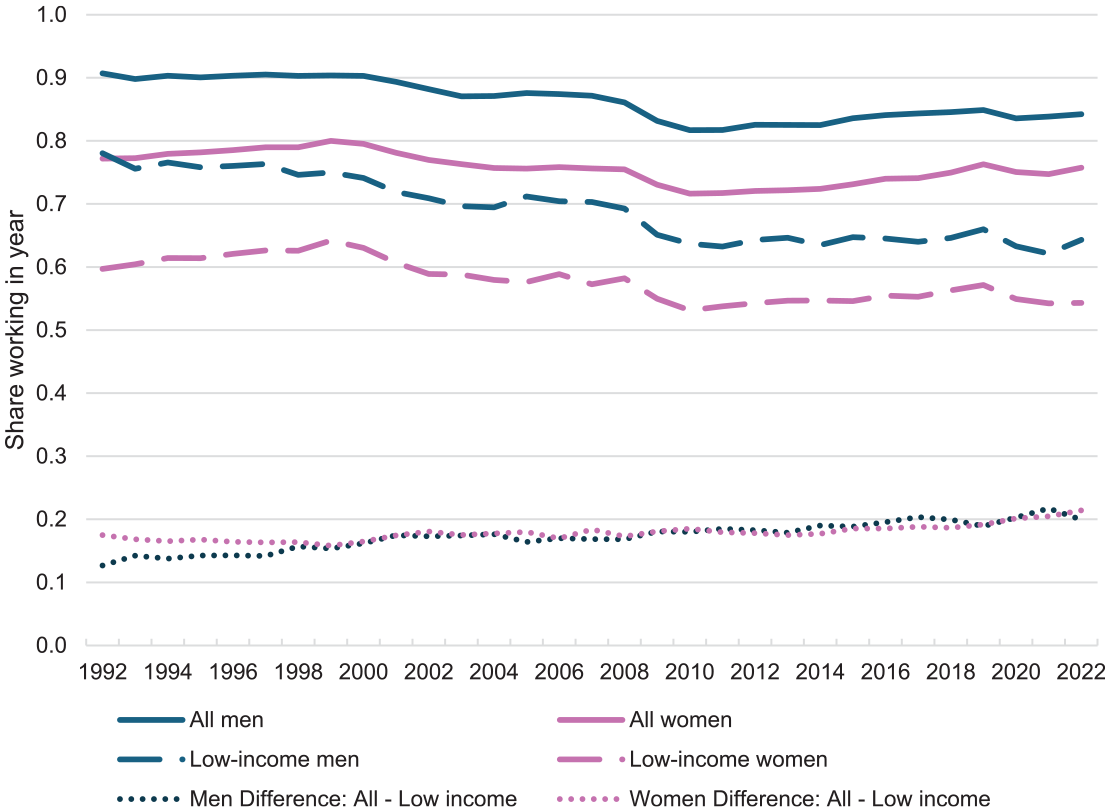
Men’s and Women’s Employment over Time: Overall, Low-Income People, and the Difference

Employment patterns are somewhat different if children are present in the household. Women with children—especially young children not yet old enough to attend school—have traditionally been less likely to be employed, in part because they are more likely to spend time caring for children (Cascio 2009; Cascio and Schanzenbach 2013). On the other hand, men with children typically are more likely to be employed than are childless men. In Figure 2a and 2b, we present employment rates for women and men, respectively, by the presence of children in their family. We note, however, that the presence of a child in the family does not mean that the adult is necessarily the child’s parent. Similarly, some adults in families without children may be parents of children who live elsewhere. Not only do employment levels and trends differ by gender and the presence of children, but they also differ between the overall and low-income samples.

Figure 2

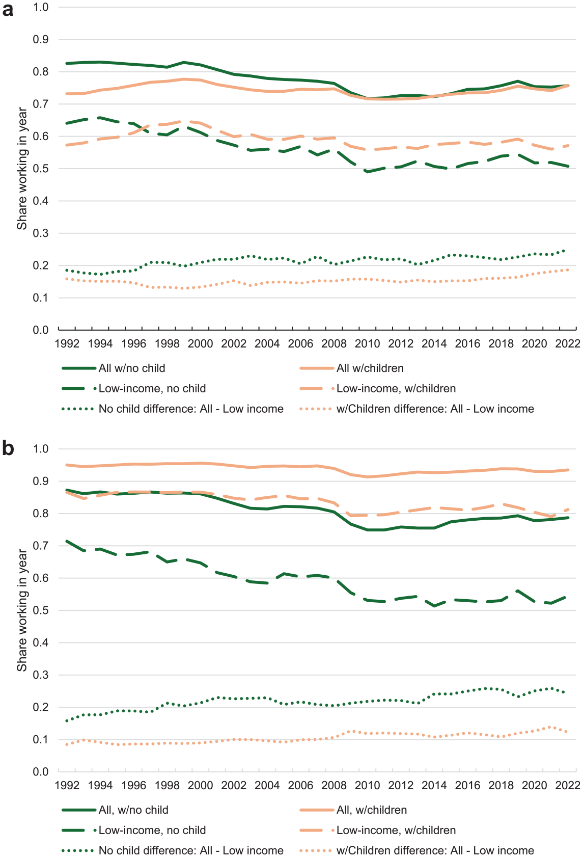
(a) Women’s Employment over Time, by Income Status and Presence of Children. (b) Men’s Employment over Time, by Poverty Status and Presence of Children.

Women’s employment rates are shown in Figure 2a. Women with children—both overall (light solid line) and among the low-income sample (light dashed line)—were increasingly likely to work between 1992 and 1999. On the other hand, women without children overall (dark solid line) and in low-income families (dark dashed line) had employment rates that were flat or declining over this period. By 1998, low-income women with children were more likely to be employed than low-income, childless women were—a pattern that held for the subsequent 20 years.

From 1999 to 2010, all four groups of women had declining employment, but childless women’s employment rate was dropping faster than that of women with children. In the overall sample, employment rates between women with children and childless women had converged by 2010, and their employment rates have tracked each other since. The differences in employment rates between women overall and low-income women have increased for women with children (light dotted line) and without children (dark dotted line) but have grown more among childless women. As we discuss below, some of these differences in trends may reflect responses to social benefits programs that are generally more generous to low-income women with children than other groups (Hoynes and Rothstein 2017).

Figure 2b shows employment rates among men over time. Overall, almost all men with children are employed. From 1992 through 2007, employment rates hovered around 95 percent before declining to 91 percent in 2010 during the aftermath of the Great Recession and rebounding to 94 percent by the late 2010s (light solid line). Low-income men with children were employed at lower levels but generally followed a similar pattern over time, with employment rates around 85 percent prior to the Great Recession, hitting a trough of 79 percent, and then rebounding to 82 percent in the late 2010s (light dashed line). Overall, trends in employment among men with children have been similar over time between the overall population and the low-income groups; the gap in employment rates between men with children overall and those with low incomes (light dotted line) hovered around 10 percentage points prior to the Great Recession and increased to around 12 percentage points in the 2010s.

Among childless men, however, employment rates have fallen over time, and by a larger amount among the low-income group. Employment rates among childless men overall (dark solid line) fell from 87 percent in 1992 to a low of 75 percent during the Great Recession before rebounding to 79 percent in the late 2010s. Employment rates among low-income, childless men (dark dashed line) have declined much more rapidly, falling from 71 percent to rates in the low 50s and showing little to no increase during periods of rapid economic expansion (including the years prior to the Great Recession and the 2010s). The gap between childless men overall and those in the low-income sample (dark dotted line) has grown from about 16 percentage points to about 25 percentage points over the entire period.

It is worth noting that the link between men’s employment status and the presence of children likely runs both ways. That is, while men surely may be more likely to work because they have children to support, it is also likely that fathers who are unemployed may be more likely to divorce or less likely to marry and thus less likely to live with their children. Further, the strength of the forces relating employment to living arrangements may be changing over time.

In summary, low-income men and women both with and without children have employment patterns that generally follow the corresponding population overall, but the differences between employment rates overall and among low-income adults generally have been increasing over time. One additional notable finding is that low-income women with children are now more likely to be employed than are low-income women without children.

Trends in Demographic Characteristics of the Low-Income Population

In addition to gender and whether one has children, other factors influence the likelihood that someone is employed, including age, marital status, education level, immigrant status, and race and ethnicity. In Table 1, we show a range of economic and demographic characteristics among the low-income population (with family income below 200 percent of the poverty line) ages 18 to 54 and the ways in which those characteristics have changed over time. Columns 2 through 5 provide snapshots of characteristics every decade from 1992 through 2022. Column 1 reproduces a portion of a similar table in Blank, Danziger, and Schoeni (2006a) showing (where available) the same characteristics in 1979.

In 1979 and 1992, about 68 percent of low-income adults were employed. This share fell to 59 percent in 2012 and was the same in 2022. Inflation-adjusted median family income among the low-income population fluctuated over time, likely because of changes in the macroeconomy. Among the low-income population, real median income increased from around $21,500 in 1992 to just above $24,000 in 2002; it dropped somewhat to $22,711 in 2012 and increased to $25,006 in 2022. As a share of the total population ages 18 to 54, between one-quarter and one-third lived in households with incomes less than 200 percent of the poverty threshold—again likely because of overall economic conditions (bottom row of Table 1). The share of the low-income population that is female held steady over time at about 55 percent, and the average age edged up from 32.7 years to 34.0 years. (Note that Blank, Danziger, and Schoeni [2006a] did not report age or share female in 1979.)

There has been a sizable shift in the family composition among low-income adults over time. In 1979, 57 percent were married; but by 2022, only 32 percent were married, and 23 percent were married with children (down from 35 percent in 1992). The share of the low-income population that is unmarried with children grew from 19 percent in 1979 to 25 percent in 1992 and has remained more or less steady since then. The share of the low-income population without children has increased steadily over time, from 40 percent in 1992 to 52 percent in 2022. In summary, by 2022, about half of the low-income population was childless, and the half living with children was split about equally between those who are married and those who are unmarried.

The racial and ethnic composition of the low-income population has also shifted substantially. The share of the low-income population that is white (not Hispanic) fell sharply from 69 percent in 1979 and 57 percent in 1992 to 42 percent in 2022, and the share of the low-income population that is Black (not Hispanic) fell somewhat from 21 percent to 17 percent. The share that is Hispanic (of any race) tripled over this time period, from 10 percent in 1979 to 32 percent in 2022. Immigrant status is not available for all years in the CPS ASEC data, but from 2002 to 2022, around a quarter of the low-income adult population were immigrants. In some cases, social safety net benefits are not available to immigrants, and participation among eligible immigrants is lower than among the native-born population (Bitler, Hoynes, and Schanzenbach 2023; Butcher, Hu, and Perry, this volume). As a result, the impact of these programs on employment and family well-being may differ across racial and ethnic groups or over time as these populations shift. Overall, in 2022, almost one-third of the low-income population was Hispanic, just under one-fifth was Black, and just over two-fifths was white.

Education levels of low-income adults have increased over this period, with the share lacking a high school diploma dropping from 40 percent in 1979 to 30 percent in 1992 and to 20 percent by 2022. The share with some college or more increased over time from 26 percent in 1979 and 28 percent in 1992 to 38 percent in 2022; over this period, the share with a bachelor’s degree or higher more than doubled. Since those with higher levels of education are more likely to be employed, all else equal, increased education levels should lead to higher employment rates. In the low-income population in 2022, about one in five adults did not have a high school diploma, just over two in five were high school graduates, and just under two in five had some college or more.

Understanding the Patterns in Employment Among the Low-Income Population

Since it is well-known that characteristics such as marital status, the presence of children, and so on influence the likelihood of being employed, a natural question to ask is how much of the change in employment among the low-income population can be explained by changes in population characteristics? Furthermore, to the extent that the low-income population has experienced increases in characteristics that are positively associated with employment (such as increased educational attainment), how much larger would the decline in employment have been if these increases had not occurred?

To address these questions, we conduct a series of Oaxaca-Blinder decompositions (see the online appendix for a more technical description of the method and detailed regression results). Using the time series of employment for low-income women with children, we select three periods of time for analysis—1992 to 1999, 1999 to 2010, and 2010 to 2019—based on the fact that 1999, 2010, and 2019 mark points at which we see a change in the direction of the trends in employment rates. We run a series of ordinary least squares regression models of the following form:

E m p l o y e d_{i} = a + A g e_{i} β + F a m C o m p_{i} γ + R a c e E t h_{i} δ + E d u c_{i} η + ε_{i} .

Each regression is run separately by year (1992, 1999, 2010, 2019) and by gender and includes only the population with family income under 200 percent of the poverty threshold. The dependent variable, Employed_i, is an indicator for whether the individual was employed at any time in the year. The group of variables Age_i includes age in years and age in years squared to account for the curved relationship between age and employment, where the likelihood of employment generally increases over young ages as people finish school and join the workforce and decreases over older ages as some opt for early retirement. FamComp_i includes indicator variables for whether the individual is married, whether there is a child under age 18 in the family, and the interaction of these two (i.e., whether the individual is married with children). RaceEth_i includes indicator variables for whether the individual is Hispanic (of any race), Black (not Hispanic), or “other” (not Hispanic, Black, or white). Educ_i includes indicator variables for whether the individual has less than a high school diploma, is exactly a high school graduate, or has attended some college. In general, those with higher levels of education are more likely to be employed. The estimated coefficients (represented above by the vectors β, γ, δ and η) tell us how much more (or less) likely a person is to work, holding other factors constant, if they have the characteristic indicated—for example, they are married or are a high school graduate.

Our Oaxaca-Blinder decomposition makes a series of comparisons of regressions run on data from different years. Take the example of employment among low-income men in 1992 and 1999. In 1992, 78.0 percent of men in the sample were employed. By 1999, 75.0 percent were—a difference of 3 percentage points. How much of this 3-percentage-point decline can we explain by changes in characteristics among low-income men over this period?

The coefficients from the 1992 regression indicate that men with less than a high school diploma were 12.6 percentage points less likely to be employed than college graduates, and married men were 9.3 percentage points more likely to be employed relative to unmarried men. The first thought experiment in the Oaxaca-Blinder decomposition is, What would the predicted employment rate be if we took the characteristics of men in 1999 and used the coefficients from 1992 to make the prediction? In other words, between 1992 and 1999, men were less likely to be married and less likely to be high school dropouts. As a result, we would expect that fewer dropouts would lead to more employment, but we would also expect that fewer married men would lead to less employment. We do this thought experiment with all of the characteristics included in the regression and predict that 77.0 percent of men would be employed in 1999 based on the relationships between characteristics and employment that existed in 1992. In other words, based on changes in the characteristics of men over time, alone, we would have expected employment to drop from 78.0 percent in 1992 to 77.0 percent in 1999. While we expected a 1-percentage-point drop, the actual decline was 3 percentage points, so one-third of the decline can be “explained” by changes in characteristics.

A second thought experiment is, How much of the difference over time can be attributed to changes in the relationship between characteristics and employment? In the 1992 regression, married men were 9.3 percentage points more likely to be employed than unmarried men were. In 1999, however, married men were only 7.0 percentage points more likely to be employed. Those with less than a high school diploma were 12.6 percentage points less likely to be employed in 1992 but only 8.3 percentage points less likely in 1999. While we do not know what caused these relationships to change over time, we can nonetheless estimate how much of the 3-percentage-point drop in employment that occurred can be explained by changes in the relationship (i.e., the coefficients) between the explanatory characteristics and employment over time. Here, 2.1 percentage points of the drop can be accounted for by changes in coefficients over time. (A small amount is due to the interaction between characteristics and coefficients, and the numbers do not add perfectly due to rounding.)

The consolidated results of the Oaxaca-Blinder decompositions are shown in Table 2, and regression coefficients are in the online appendix. Columns 1 and 2 show results for men and women comparing 1992 to 1999. As described in the paragraphs above, men’s employment fell by 3 percentage points over this period, with one-third of the decline explained by changes in characteristics among low-income men over this period and two-thirds “unexplained” and attributed in an accounting sense to changes in the regression coefficients across years. In contrast to men’s, women’s employment increased over this period by 4.5 percentage points. Essentially none of the increase is explained by changes in characteristics among low-income women; it is instead accounted for by changes in coefficients. For example, in 1992, low-income women with children at home were 6.6 percentage points less likely to be employed than low-income women without children, conditional on other factors; by 1999, low-income women with children were 5.8 percentage points more likely to be employed than similar women without children. Consistent with this change in coefficients, during this time frame, policy changes expanding the EITC increased low-income mothers’ incentives to work.

Table 2

Explaining Changes in Employment Rates, Oaxaca-Blinder Decomposition Results

	1992 to 1999		1999 to 2010		2010 to 2019
	Men	Women	Men	Women	Men	Women
	(1)	(2)	(3)	(4)	(5)	(6)
Mean: Later year	0.750*** (0.006)	0.642*** (0.005)	0.637*** (0.005)	0.531*** (0.004)	0.660*** (0.007)	0.571*** (0.006)
Mean: Earlier year	0.780*** (0.005)	0.597*** (0.005)	0.750*** (0.006)	0.642*** (0.005)	0.637*** (0.005)	0.531*** (0.004)
Employment rate difference	−0.030*** (0.007)	0.045*** (0.007)	−0.113*** (0.007)	−0.111*** (0.007)	0.023*** (0.008)	0.040*** (0.007)
Difference due to characteristics	−0.010*** (0.002)	0.003 (0.002)	−0.020*** (0.003)	−0.004 (0.002)	−0.002 (0.003)	0.010*** (0.002)
Difference due to coefficients	−0.021*** (0.007)	0.047*** (0.007)	−0.096*** (0.007)	−0.114*** (0.007)	0.028*** (0.008)	0.027*** (0.007)
Difference: interaction of characteristics & coefficients	0.000 (0.002)	−0.005** (0.002)	0.003 (0.002)	0.007*** (0.002)	−0.002 (0.002)	0.003* (0.002)
% of difference explained by characteristics	33%	7%	18%	4%	—	25%
% of difference unexplained	67%	93%	82%	96%	>100%	75%

SOURCE: Authors’ calculations from CPS ASEC surveys, 1993, 2000, 2011, and 2020.

NOTE: Sample is limited to adults ages 18 to 54 living in families with total pretax income and losses less than 200 percent of the official poverty cutoff. Characteristics include measures of age, family composition, race and ethnicity, and education.

p < .10, **p < .05, ***p < .01.

Between 1999 and 2010, both women’s and men’s employment rates fell by 11 percentage points. Very little of this decline is explained by changes in population characteristics. For example, less than 20 percent of the decline among men can be explained by changes in characteristics; the primary explanatory factor was increased age. Less than 4 percent of the decline in women’s employment can be explained by changes in population characteristics.

During the period of economic expansion from 2010 to 2019, employment rates increased among low-income men by 2.3 percentage points and among low-income women by 4.0 percentage points. One-quarter of the increase in low-income women’s employment can be explained by changes in population characteristics, while essentially none of the increase in low-income men’s employment is related to changes in population characteristics.

We present all the regression coefficients in the online appendix, and there are some interesting changes in the regression coefficients over time worth highlighting. Among women, in 1992 and 1999, there were sizable, statistically significant coefficients on the indicators for whether the individual is Hispanic, Black, or of “other” racial group, relative to whites. That these coefficients were small and statistically insignificant in 2019 indicates that, conditional on the other factors included in the regression, there were no differences in employment rates across racial and ethnic groups. Further, although women with lower levels of education were less likely to be employed than those with higher levels of education, the size of the relationship declined over time. For example, in 1992, high school dropouts were nearly 26 percentage points less likely to be employed than college graduates, all else equal. By 2019, the coefficient dropped to 12 percentage points.

Among men, the coefficients on racial and ethnic group indicators do not become insignificant as they do among women. The coefficients on educational attainment, however, go from strong and aligned with expectations (i.e., high school dropouts are less likely to be employed than high school graduates, and college graduates are most likely to be employed, all else equal) to small and not individually significant in 2019. Married men were steadily more likely to be employed, with coefficients ranging from 7 to 9 percentage points over time, but the coefficients on men who were married with children increased over time from 9 percentage points in 1992 to 16 percentage points in 2019.

One conclusion that we can draw from these findings is that shifting characteristics of the population explain relatively little of the pattern in employment changes. Two notable exceptions are that changes in men’s characteristics explain a third of their employment decline from 1992 to 1999, and changes in women’s characteristics explain about a quarter of their increase from 2010 to 2019.

Almost all the large decline in employment rates between 1999 and 2010 is unexplained by factors included in the regressions. These findings, combined with the similar-sized drop in employment among the overall population shown in Figure 1, suggest that broader economic factors (e.g., macroeconomic conditions and policies affecting all workers—not just those with low incomes) may have been at work in those years. Similarly, relatively little of the increase in employment rates from 2010 to 2019 among the low-income population can be explained by factors included in the regressions, and these increases also largely track increases among the overall population. On the other hand, the patterns over the 1992 to 1999 period suggest that policy aimed at low-income workers may be driving some of those changes. During this period, men’s and women’s employment moved in different directions—women’s employment increased, while men’s decreased. Further, the increase in women’s employment occurred only among women with children and not childless women. Next, we will investigate safety net programs and their changes over these time periods.

Changes in Social Benefits over Time

The composition of the social benefits has changed over the past 30 years, with major policy changes during the 1990s. First, the EITC was dramatically expanded (phased in between 1993 and 1996), providing an increased benefit to employment among workers with children and low earnings (Nichols and Rothstein 2016; Schanzenbach and Strain 2021). The 1996 Personal Responsibility and Work Opportunities Reconciliation Act (PRWORA), which “ended welfare as we know it,” imposed time limits on the receipt of cash welfare and turned the program into a block grant to states that could be used for a range of activities (Bitler and Hoynes 2016). The Child Tax Credit (CTC) was introduced in 1997, was expanded and made partially refundable in 2001, and was further increased in 2012 and 2017 (Hoynes and Rothstein 2017).

Figure 3a and 3b shows how income from social benefits (as reported in the CPS ASEC) has changed over time for adults living in families with incomes less than 200 percent of the poverty threshold. (Recall that we use the official poverty measure to draw the 200 percent line, so income from some of these safety net sources are not included in the income measure; see Johnson et al. [this volume] for more details about how income is counted in various poverty measures.) We highlight income from the EITC, the Supplemental Nutrition Assistance Program (SNAP), cash welfare, Supplemental Security Income, Social Security, Unemployment Insurance (UI), and child tax credits (including both the CTC and the Additional Child Tax Credit [ACTC]). The “other” category includes workers’ compensation, veterans’ benefits, survivors’ benefits, disability insurance payments, and government education benefits (such as Pell Grants). Although SNAP is a food voucher, we count SNAP benefits at their face-value cash equivalent. We note that it is well-documented that the CPS ASEC has substantial measurement error when it comes to measuring participation in social benefit programs and the amount received from these sources (Meyer, Mok, and Sullivan 2015), and as a result, these findings should be interpreted with caution.

Figure 3

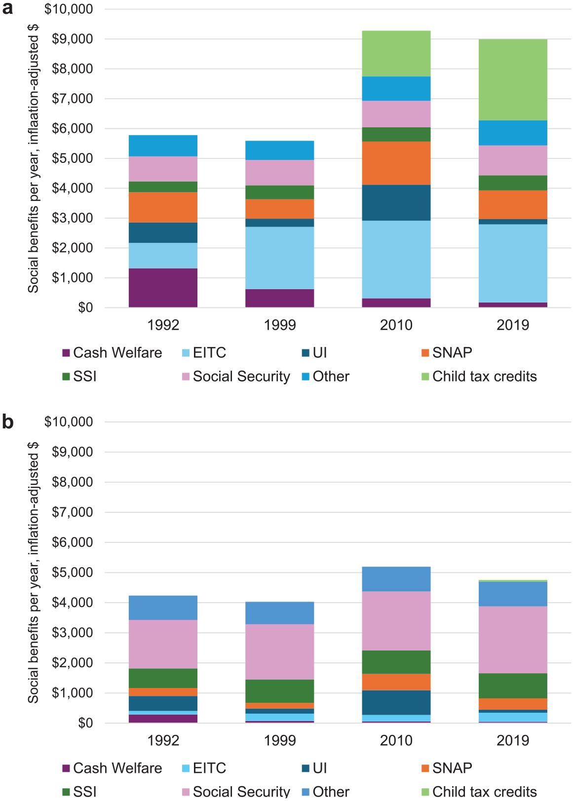
(a) Annual Income from Social Benefits over Time, Low-Income Adults with Children. (b) Annual Income from Social Benefits over Time, Low-Income Adults without Children.

Figure 3a shows the average inflation-adjusted value of benefits for low-income adults with children over time, by category. In 1992 and 1999, low-income adults with children received between $5,500 and $6,000 per year in benefits. In 2010 and 2019, the average value of benefits had increased to around $9,000 per year. While cash welfare accounted for nearly one-quarter of social benefits in 1992, by 2010, it accounted for less than 5 percent of average total benefits for low-income adults with children. This reflects in part a sharp decline in the share of low-income adults receiving any cash welfare, from 20 percent in 1992 to 4 percent in 2019. In contrast, expansion of the EITC increased both the share of low-income individuals with children receiving EITC benefits and the value of those benefits. Between 1992 and 2019, the share of low-income adults with children who reported receiving EITC increased from 59 percent to 75 percent, a 27 percent increase. Over that same period, the average value of EITC benefits more than tripled from around $850 in 1992 to $2,600 in 2019.

Changes over time in the average value of UI and SNAP benefits are related to changes in the business cycle and the share of individuals receiving these benefits (Bitler, Hoynes, and Kuka, this volume; Ganong and Liebman 2018). 1992 and 2010 represent years when the unemployment rates were reaching their highest levels in their respective business cycles. In contrast, 1999 and 2019 were low unemployment years near the peaks of their respective business cycles. During the high unemployment years of 1992 and 2010, 13 percent of these low-income individuals were receiving UI benefits, and around 30 percent reported receiving SNAP benefits. In 1999, 7 percent of individuals reported receiving UI benefits, and 20 percent reported receiving SNAP. During the business cycle peak of 2019, only 3 percent of individuals reported receiving any UI benefits, and 26 percent reported receiving SNAP. These changes in receipt are reflected in the average value of benefits received with notably more UI and SNAP receipt in 2010 than in other years shown. In 2010, average UI benefits were around $1,200, and average SNAP benefits were nearly $1,500. Average UI benefits in 2019 totaled only $176, while SNAP benefits were $962. Importantly, the CTC and ACTC (the refundable portion of the CTC) programs, which were added between 1999 and 2010, represent a large share of the increase in average total benefits. In 2019, 30 percent of benefits came from these CTCs, and 75 percent of individuals reported receiving any benefits from the ACTC.

Figure 3b repeats the exercise for individuals with no children. Notably, average total social benefits are lower for low-income adults without children, and Social Security benefits are relatively more important. The EITC benefit for childless adults is relatively modest; although the share receiving the EITC increased from 7 percent to 25 percent over this period, EITC benefits as a share of total benefits was only 6 percent in 2019. In contrast, across all years, roughly 15 percent of low-income, childless adults report receiving Social Security benefits, with the average value of benefits rising from around $1,600 to around $2,000. As a result, Social Security benefits account for nearly 50 percent of the total social benefits received by low-income, childless adults.

While Figure 3a and 3b shows the average value received from social benefits programs among low-income families, Figure 4a and 4b gives a sense of how the distributions of these benefits have shifted over time away from benefits available to nonworkers to benefits available only to those with earned income (Hoynes and Schanzenbach 2018). In Figure 4a and 4b, total family income from work is on the horizontal axis, and social benefits as a share of total income (from social benefits plus work and any other sources of income) is on the vertical axis. We limit the sample to individuals with positive total income and cap the share received from social benefits programs at one. Each dot represents the average share of income from social benefits among adults within a narrow range of family labor income, with each grouping designed to represent about 5 percent of the sample population. The location on the horizontal axis is the midpoint income within the bin, and the different shaped markers represent different survey years. Note that this approach holds labor income constant across those years. Since we have already seen that a changing share of adults are employed over time, the number of people with zero labor income varies somewhat across years (22 percent of individuals have family earned income equal to zero in 1992, compared with 26 percent of individuals in 2019).

Figure 4

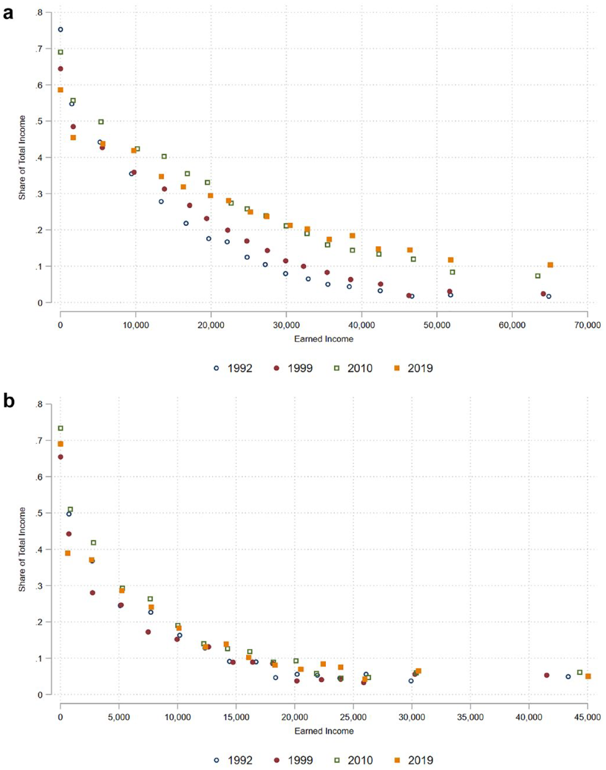
(a) Share of Income from Social Benefits over Time, Low-Income Adults with Children. (b) Share of Income from Social Benefits over Time, Low-Income Adults without Children.

Figure 4a is limited to low-income individuals with children. In 1992, adults with the lowest family income from work on average received about 75 percent of their total income from social benefits. By tracing the open blue circles across the income distribution, we can see how the share of income from benefits changes as income increases across families in 1992. The average share of income from benefits declines sharply as income from work increases, reaching an average of less than 10 percent among those earning $30,000 or more in the year. Over time, the relationship between share of income from social benefits and family earned income becomes flatter. In 1999, those in the two lowest earnings categories received a smaller share of their total income from social benefits than was the case in 1992, and those with higher work income received a higher share of their total income from social benefits compared with 1992. This is consistent with a shift in social benefits programs to provide more benefits to those who are employed, such as the expansion of the EITC. By 2010, the share of income from benefits had moved higher for those with more labor income, most noticeably those with $20,000 or more in earnings in the year. The relationship is little changed between 2010 and 2019, a period during which there were few changes to social benefits programs.

Figure 4b shows data for low-income adults without children. Compared to households with children, we make two salient observations. First, there is little difference across years, reflecting that there has been relatively little change in the design or generosity of social benefits available to childless adults over this period. Second, the share of income from social benefits declines very quickly as labor income increases, averaging around 10 percent or less after annual labor income reaches $10,000. This finding reflects that there are few and modest benefits available to nonelderly, childless adults, and those that are available are narrowly targeted at the very poorest individuals.

In results not shown, we repeat the exercises in Figures 3 and 4 separately for men and women (with and without children). The patterns for both the mean and the distribution of benefits shares are nearly identical for childless men and women. On the other hand, among adults with children, cash welfare and SNAP payments make up a larger share of total social benefits for women than they do for men. When conditioned on earnings as in Figure 4, though, the gender differences among families with children are essentially zero.

Summary and Conclusions

Many researchers have investigated the causal impacts of changes in social benefits on employment, earnings, and poverty, and they have sometimes focused on narrow groups of people (Bitler, Gelbach, and Hoynes 2003, 2006; Blank 2002; East 2018; Hoynes and Patel 2018; Hoynes and Schanzenbach 2012). These generally find that people respond to the incentives built into these programs in the expected direction, but to varying magnitudes. In this article, we step back and take a broader view that situates employment trends among low-income people within aggregate employment trends. We find that low-income employment tracks overall employment within demographic groups defined by gender and the presence of children.

We find that characteristics of low-income adults have changed over time. They have become more highly educated and less likely to be married, and the share that is Hispanic has increased. In investigating the extent to which these shifts in characteristics can help explain changes in employment, we find that little of that change can be explained by these factors.

We also find that different social benefits programs are important for low-income, childless adults compared with those with children. While social benefits programs have become more generous to low-income adults with children who have substantial earnings, they have remained relatively stable for childless adults. As expected, UI is more important for those with and without children during economic downturns (i.e., 1992 and 2010 in these figures).

Our results contribute to a growing literature documenting the shift in the structure of social benefits for nonelderly adults, especially those with children, to reward and encourage work. Low-income families with children and substantial earnings received more income—both in levels and as a share of their total incomes—from social benefits in the past decade than they did 30 years ago. On the other hand, social benefits programs are little changed for low-income families without children.

These patterns raise certain policy questions: To what extent can (and should) social benefits programs compensate low-income workers when they face periods of stagnant wage growth? Are we providing adequate protection to those who face seemingly insurmountable barriers to employment? To what extent will the downward long-term trend in employment both overall and among the low-income population continue, and how will that impact the effectiveness of an increasingly work-based safety net? As we continue to work for a better understanding of the nature of labor supply and labor demand for adults in low-income families, addressing these questions will help us design more effective policies.

Supplemental Material

sj-docx-1-ann-10.1177_00027162241290105 – Supplemental material for Work, Poverty, and Social Benefits over the Past Three Decades

Supplemental material, sj-docx-1-ann-10.1177_00027162241290105 for Work, Poverty, and Social Benefits over the Past Three Decades by Leslie McGranahan, Diane W. Schanzenbach, Lisa Barrow, Diane W. Schanzenbach and Bea Rivera in The ANNALS of the American Academy of Political and Social Science

Footnotes

Supplemental Material

Supplemental material for this article is available online.

Notes

Lisa Barrow is vice president of regional analysis in the research department of the Federal Reserve Bank of Cleveland. She is a labor economist who specializes in education topics. She served as senior economist at the Council of Economic Advisers from 2021 to 2022.

Diane W. Schanzenbach is Margaret Walker Alexander Professor in Education and Social Policy and a faculty fellow in the Institute for Policy Research at Northwestern University. She is a research associate of the National Bureau of Economic Research and an elected member of the National Academy of Education.

Bea Rivera is an associate in the labor and employment practice at Charles River Associates. She was formerly a research assistant at the Federal Reserve Bank of Chicago.

References

Abraham

Katharine G.

Kearney

Melissa S.

. 2020. Explaining the decline in the U.S. employment-to-population ratio: A review of the evidence. Journal of Economic Literature 58(3): 585–643.

Acs

Gregory

Nichols

Austin

. 2007. Low-income workers and their employers: Characteristics and challenges. Washington, DC: Urban Institute. Available from www.urban.org.

Bahk

Sung Ah

Moffitt

Robert

Smeeding

Timothy M.

. 2024. Legacies of the War on Poverty. The ANNALS of the American Academy of Political and Social Science 711: 38–56.

Bitler

Marianne P.

Gelbach

Jonah B.

Hoynes

Hilary W.

. 2003. Some evidence on race, welfare reform, and household income. American Economic Review 93(2): 293–298.

Bitler

Marianne P.

Gelbach

Jonah B.

Hoynes

Hilary W.

. 2006. What mean impacts miss: Distributional effects of welfare reform experiments. American Economic Review 96(4): 988–1012.

Bitler

Marianne

Hoynes

Hilary

. 2015. Heterogeneity in the impact of economic cycles and the Great Recession: Effects within and across the income distribution. American Economic Review 105(5): 154–160.

Bitler

Marianne

Hoynes

Hilary

. 2016. Strengthening Temporary Assistance for Needy Families. Policy Proposal 2016-04. Washington, DC: The Hamilton Project. Available from https://www.brookings.edu/wp-content/uploads/2023/01/20160520_THP_bitler_hoynes_strengthening_tanf.pdf.

Bitler

Marianne P.

Hoynes

Hilary

Kuka

Elira

. 2024. The macroeconomy and poverty. The ANNALS of the American Academy of Political and Social Science 711: 82–99.

Bitler

Marianne P.

Hoynes

Hilary W.

Schanzenbach

Diane Whitmore

. 2023. Suffering, the safety net, and disparities during COVID-19. RSF: The Russell Sage Foundation Journal of the Social Sciences 9(3): 32–59.

10.

Black

Sandra E.

Schanzenbach

Diane Whitmore

Breitwieser

Audrey

. 2017. The recent decline in women’s labor force participation. In The 51%: Driving growth through women’s economic participation, eds. Schanzenbach

Diane Whitmore

Nunn

Ryan

, 5–17. Washington, DC: The Hamilton Project.

11.

Blank

Rebecca M.

2002. Evaluating welfare reform in the U.S. Journal of Economic Literature 40(4): 1105–1166.

12.

Blank

Rebecca M.

Danziger

Sheldon H.

Schoeni

Robert F.

. 2006a. Introduction: Work and poverty during the past quarter-century. In Working and poor: How economic and policy changes are affecting low-wage workers, eds. Blank

Rebecca M.

Danziger

Sheldon H.

Schoeni

Robert F.

, 1–20. New York, NY: Russell Sage Foundation.

13.

Blank

Rebecca M.

Danziger

Sheldon H.

Schoeni

Robert F.

. 2006b. Working and poor: How economic and policy changes are affecting low-wage workers. New York, NY: Russell Sage Foundation.

14.

Butcher

Kristin F.

Luojia

Perry

Ryan

. 2024. The public charge rule and program participation among U.S. citizens. The ANNALS of the American Academy of Political and Social Science 711: 170–198.

15.

Butcher

Kristin F.

Schanzenbach

Diane Whitmore

. 2018. Most workers in low-wage labor market work substantial hours, in volatile jobs. Washington, DC: Center on Budget and Policy Priorities. Available from www.cbpp.org.

16.

David

Card

Blank

Rebecca M.

, eds. 2000. Finding jobs: Work and welfare reform. New York, NY: Russell Sage Foundation.

17.

Cascio

Elizabeth U.

2009. Maternal labor supply and the introduction of kindergartens into American public schools. Journal of Human Resources 44(1): 140–170.

18.

Cascio

Elizabeth U.

Schanzenbach

Diane Whitmore

. 2013. The impacts of expanding access to high-quality preschool education. Brookings Papers on Economic Activity (Fall): 127–178. https://www.jstor.org/stable/23723436

19.

Cengiz

Doruk

Dube

Arindrajit

Lindner

Attila

Zipperer

Ben

. 2019. The effect of minimum wages on low-wage jobs. Quarterly Journal of Economics 134(3): 1405–1454.

20.

Clemens

Jeffrey

Strain

Michael R.

. 2021. The heterogeneous effects of large and small minimum wage changes: Evidence over the short and medium run using a pre-analysis plan. National Bureau of Economic Research Working Paper 29264, Cambridge, MA.

21.

Cook

Jason B.

East

Chloe N.

. 2024. Work requirements with no teeth still bite: Disenrollment and labor supply effects of SNAP general work requirements. National Bureau of Economic Research Working Paper 32441, Cambridge, MA.

22.

Council of Economic Advisers. 2016. The long-term decline in prime-age male labor force participation. Washington, DC: Council of Economic Advisers, Executive Office of the President of the United States. Available from obamawhitehouse.archives.gov.

23.

Dillender

Marcus

Heinrich

Carolyn J.

Houseman

Susan

. 2022. Effects of the Affordable Care Act on part-time employment: Early evidence. Journal of Human Resources 57(4): 1394–1423.

24.

East

Chloe N.

2018. Immigrants’ labor supply response to Food Stamp access. Labour Economics 51: 202–226.

25.

Flood

Sarah

King

Miriam

Rodgers

Renae

Ruggles

Steven

Warren

J. Robert

Backman

Daniel

Chen

Annie

Cooper

Grace

Richards

Stephanie

Schouweiler

Megan

Westberry

Michael

. 2023. IPUMS CPS: Version 11.0 [dataset]. Minneapolis, MN: IPUMS. Available from cps.ipums.org.

26.

Gabe

Todd

Abel

Jaison R.

Florida

Richard

. 2018. Can low-wage workers find better jobs? Staff Report 846. New York, NY: Federal Reserve Bank of New York. Available from www.newyorkfed.org.

27.

Ganong

Peter

Liebman

Jeffrey B.

. 2018. The decline, rebound, and further rise in SNAP enrollment: Disentangling business cycle fluctuations and policy changes. American Economic Journal: Economic Policy 10(4): 153–176.

28.

Hoynes

Hilary W.

2000. The employment, earnings, and income of less skilled workers over the business cycle. In Finding jobs: Work and welfare reform, eds. Card

David

Blank

Rebecca M.

, 23–71. New York, NY: Russell Sage Foundation.

29.

Hoynes

Hilary W.

Patel

Ankur J.

. 2018. Effective policy for reducing poverty and inequality? The Earned Income Tax Credit and the distribution of income. Journal of Human Resources 53(4): 859–890.

30.

Hoynes

Hilary

Rothstein

Jesse

. 2017. Tax policy toward low-income families. In The economics of tax policy, eds. Auerbach

Alan J.

Smetters

Kent

, 183–225. New York, NY: Oxford University Press.

31.

Hoynes

Hilary Williamson

Schanzenbach

Diane Whitmore

. 2012. Work incentives and the food stamp program. Journal of Public Economics 96(1–2): 151–162.

32.

Hoynes

Hilary W.

Schanzenbach

Diane Whitmore

. 2018. Safety net investments in children. Brookings Papers on Economic Activity (Spring): 89–132. https://www.jstor.org/stable/26506214

33.

Jardim

Ekaterina

Long

Mark C.

Plotnick

Robert

van Inwegen

Emma

Vigdor

Jacob

Wething

Hilary

. 2022. Minimum-wage increases and low-wage employment: Evidence from Seattle. American Economic Journal: Economic Policy 14(2): 263–314.

34.

Johnson

David S.

Levy

Helen

Matsudaira

Jordan

Wolfe

Barbara L.

Ziliak

James P.

. 2024. Measuring poverty: Advances to the Supplemental Poverty Measure. The ANNALS of the American Academy of Political and Social Science 711: 20–37.

35.

Kim

Marlene

. 2000. Women paid low wages: Who they are and where they work. Monthly Labor Review 123(9): 26–30.

36.

Kuka

Elira

Shenhav

Na’ama

. 2024. Long-run effects of incentivizing work after childbirth. American Economic Review 114(6): 1692–1722.

37.

Looney

Adam

Manoli

Dayanand S.

. 2016. Are there returns to experience at low-skill jobs? Evidence from single mothers in the United States over the 1990s. Upjohn Institute Working Paper 16-255, Kalamazoo, MI.

38.

Meyer

Bruce D.

Mok

Wallace K.C.

Sullivan

James X.

. 2015. Household surveys in crisis. Journal of Economic Perspectives 29(4): 199–226.

39.

Neumark

David

Asquith

Brian

Bass

Brittany

. 2020. Longer-run effects of anti-poverty policies on disadvantaged neighborhoods. Contemporary Economic Policy 38(3): 409–434.

40.

Nichols

Austin

Rothstein

Jesse

. 2016. The earned income tax credit. In Economics of means-tested transfer programs in the United States, vol. 1, ed. Moffitt

Robert A.

, 137–218. Chicago, IL: University of Chicago Press.

41.

Schanzenbach

Diane Whitmore

Strain

Michael R.

. 2021. Employment effects of the Earned Income Tax Credit: Taking the long view. Tax Policy and the Economy 35: 87–129.

Supplementary Material

Please find the following supplemental material available below.

For Open Access articles published under a Creative Commons License, all supplemental material carries the same license as the article it is associated with.

For non-Open Access articles published, all supplemental material carries a non-exclusive license, and permission requests for re-use of supplemental material or any part of supplemental material shall be sent directly to the copyright owner as specified in the copyright notice associated with the article.

0.00 MB

0.04 MB

Work,Poverty,and Social Benefits over the Past Three Decades

Abstract

Keywords

Trends in Employment

Trends in Demographic Characteristics of the Low-Income Population

Understanding the Patterns in Employment Among the Low-Income Population

Changes in Social Benefits over Time

Summary and Conclusions

Supplemental Material

sj-docx-1-ann-10.1177_00027162241290105 – Supplemental material for Work, Poverty, and Social Benefits over the Past Three Decades

Footnotes

Supplemental Material

Notes

References

Supplementary Material