
Abstract
The present work focuses on predicting users' next place of visit using their past tweets. We hypothesize that tweets of the person have predictive power on his location and therefore can be used to predict his next place of visit. This problem is important for location based advertising and recommender based services. To predict the next place of visit, we calculate the probabilities of visiting different types of places using bank of binary classifiers and Markov models. More specifically, we train bank of binary classifiers on past tweets and calculated the probabilities of visiting next places. Since bank of binary classifiers is based on a bag-of-words model, to account for time of last visited place and place itself, we built Markov models for different time duration to calculate probabilities of visiting next place. Empirical evaluation shows that by combining the probabilities obtained from bank of binary classifiers and Markov models the accuracy of predicting next place increased from 65% to 80%.
1. Introduction
How the life would be if we know the location of desired and intended place around us anywhere in the world. Though it seems to be superficial, the development in wireless and location acquisition technology helps us to build systems that solve this problem to some extent. Because of location acquisition technology, nowadays, it is not difficult to find out the places in given proximity. The bigger challenge is in predicting places for user according to his need and intent in given proximity. The existence of microblogging services like Twitter and Facebook provides a means to know the person's values and needs in better way.
People share their thoughts and happening on Twitter along with mundane information. In recent few years, the popularity of Twitter is growing exponentially. As of now, at the time of writing this paper the number of users on Twitter are 300 million producing 500 million (https://about.twitter.com/company) tweets per day. With mundane information, people also share their activities like what they are planning, visited places, experiences of visited places, with whom they are going, how they are feeling, and so forth. Availability of such valuable information motivates us to build a system that can predict the future places of visits for the user according to their intent and behavior.
In this paper, we hypothesize that future places of visit can be predicted considering two important factors that are (i) previous visited place and (ii) recent tweets. What people write on their timeline reflects their intent and need, which have a significant role in deciding the next activity to be performed. Similarly, previous visited place also has a major role in deciding the next place to be visited. For example, after having lunch people have coffee. Based on given hypothesis we propose a novel approach for predicting next places of visit. We use bank of binary classifiers (BBC) for predicting the probability of visiting next place using recent tweets only. And to account for time of last visited place and place itself, we build Markov models (MMs) for predicting probabilities. Both BBC and MMs compute the probability of visiting next place independently with high accuracy. We show that by combining these two probabilities we can further improve the prediction accuracy. In attaining the goal of this work, we also proposed two algorithms for tagging the tweets with location and for finding out the optimum number of past tweets used for prediction. Our approach consists of the following steps: (a) assigning location to tweets if relevant information is presents; (b) extracting features from past tweets that are used to train the models; (c) building models using bank of binary classifiers; (d) using contextual information to enhance the accuracy of predicting the next place. Here contextual information is time of previous visited place and place itself.
We crawl more than 4600 Twitter timelines for exhaustive experimentation. Ground truths are extracted from these timelines using Google Places API and by analyzing tweets for mentions of visited places. We extract features from users timelines by using our proposed algorithm for finding out the optimum length of past tweets for prediction. We build models and do performance analysis. Our best model yields 80% of accuracy for top 5 predictions. We evaluate our approach on new users also and show that performances of models are similar to the seen users to model. The major contribution of this works is as follows:
Building generic models for predicting future places of visit using recent tweets only. Building Markov models for predicting next place to be visited given previous place visited and time since it is visited. Ensemble of both models to enhance the model accuracy in predicting next place.
The remainder of the paper is organized as follows. Section 2 presents the proposed approach in detail for predicting next place of visit. Next, Section 3 discusses the experiments and analysis of results. In Section 4 we review relevant literature work. Finally, Section 5 concludes the paper.
2. Proposed Approach
There are two points we want to mention before explaining the 4 steps of proposed approach. Firstly, we build the generic prediction model that captures the relationship between vocabulary used in past tweets and visited places, without considering user's demographics. The main advantage of this approach is that we do not need individual specific training data for predicting their next location.
Secondly, our focus would be the category of the establishment like restaurant, supermarket, pub, and gym, rather than the specific establishment. By doing this, both establishment owners and users can get mutual benefits. For example, if proposed system is predicting restaurant in given spatial proximity, then all the owners of restaurants in the proximity of user's location can approach user with their available offers for promotions. Along with this, the user can also have the option to choose place according to his own suitable interest.
Four steps of our proposed approach are as follows.
2.1. Assigning Location to Tweets
From here onwards we are using location and place of visit interchangeably. Assigning location to tweet is two-step process. First, filter all those tweets having geocoordinates and location information. For location information, we use a regular expression (“I'm at” or “@”). Then by using Google Places API [1] (GPA), get all the places around geocoordinates of the given tweet. If place name present in a tweet is present among places returned by GPA, then that tweet is labeled by the name and categories of location. We want to mention that GPA also returns categories of places which may be more than one. For matching the place name, we extract three words after regular expression from a tweet and find out the ratio r, with total words in each place name returned by GPA. If
2.2. Extracted Features
For predicting next place of visit, we use past tweets to infer the intent and interest of the user. We analyze from the ground truths recovered from timelines that people post activity related text before performing that activity. For example, user tweeted, “We are planning to go for some fun” before visiting the central park in New York. The time interval of activity related post may vary from weeks to hours based on the activity to be performed. For example, user interested in cricket match going to happen next month has already started tweeting about the event whereas a user interested in going to a restaurant in the evening tweets just a few hours before visiting restaurant. Therefore, we built independent binary classifiers for each category using appropriate size of the window of past tweets. Here window stands for the time window of past tweets that is to be taken to form feature vectors. The window size is found empirically for each classifier/category independently and explained in next section.
To form feature vectors, first we label past tweets (concatenation of past tweets in given window) with the categories of location, visited by the user, just after posting these past tweets. Note that the location which user has visited can have more than one category, and, therefore, the labels of past tweets may be more than one. It is worth mentioning here that while concatenating past tweets, we are not considering location tweet (tweet that has location information). To build a binary classifier for category
Toy Dataset having five instances and four different categories.
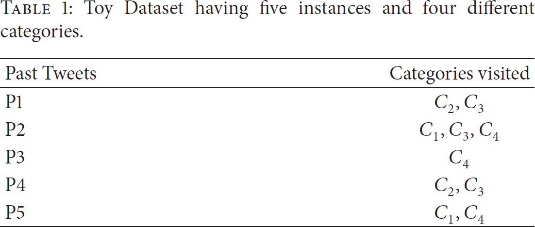
Four binary datasets constructed for each category respectively using dataset given in Table 1. Here − denotes the negative samples.

2.3. Bank of Binary Classifiers (BBC) for Predicting Future Location
For each category, we build independent binary classifier and the size of the window of past tweets for each classifier is determined empirically. The steps for determining the window size of past tweets for category
( ( ( ( ( ( ( ( ( ( ( ( ( ( ( ( ( ( ( ( (
In Algorithm 1, for each category, we vary window size w (in hours) from 6 hours to 600 hours to construct feature vectors. Then, for each window size w, we form feature vectors that are used to train the binary classifier. Finally, the window size of a particular category is set, based on the best performance of classifier among all window sizes. For constructing binary data set of each category, function getBinaryDataSet
Figure 1 shows the block diagram of prediction of places of visit using past tweets. From past tweets we form feature vector FV(

Predicting probability of visiting category
2.4. Considering Previous Visited Place and Time
We consider two other important factors in predicting next place of visit that are previously visited place and amount of time before it is visited (i.e., time duration) along with the recent tweets. For example, predicting next place of visit as restaurant, after user has visited restaurant only, within an hour, is not considered as a good prediction. For our purpose, to track the duration of time between visits of next and previous place, we discretize the time into one-hour slots. We capture the human behavior of visit in a very simplified manner by building Markov chain for different time duration. Therefore, for each time duration, we form Markov chain and transition matrix. In transition matrix 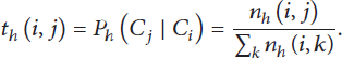
We form transition matrix for each time duration (hours) in set 
Considering independence assumption between previous visited categories we can write (2) as


In order to predict the next place of visit using past tweets and amount of time before which categories are visited by user, we combine these two probabilities that are 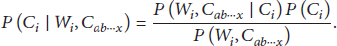
As 


3. Experiments
We have done exhaustive experiments on the data set crawled from Twitter using publicly available Twitter API. We have collected 4606 users' timelines that have tweeted at least once from New York between April 24, 2014, and April 29, 2014. Each timeline contains approximately 3200 recent tweets. Also, the tweet rate of these users is at least 20 tweets per day. Among 4606 users the number of location tweets on timelines is highly variable. Though we have started from New York the locations visited by users in our data set are around the world.
3.1. Data Sets
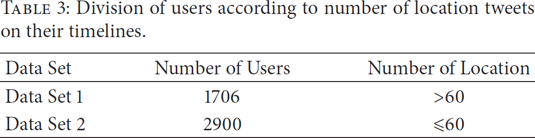
For evaluation, we divide our data set into two subsets according to the number of locations on user's timeline. Therefore, among 4606 users, those who have more than 60 location tweets (tweet that has location information) on their Twitter timeline are considered in the first subset named Data Set 1 and the remaining users in the second subset named Data Set 2. Table 3 has shown both data sets mentioned.
Division of users according to number of location tweets on their timelines.
Description of training and testing data sets.

Training Data Set (TDS). From Data Set 1, we use oldest
Testing Data Set. For evaluating the performance of models on both seen and unseen users, we use two different sets for testing, named as Test Set 1 and Test Set 2.
Test Set 1 (TS1): we use the remaining latest 50 location tweets of each user from Data Set 1 to form feature vectors. Test Set 2 (TS2): we use all location tweets from Data Set 2 to form feature vectors.
3.2. Evaluation
First we present methods to compute the accuracies of proposed models one by one in the following subsections and then propose few baselines for comparing our proposed models.
3.2.1. Using Markov Models (MMs) Only
We form transition matrix For every test instance, first we find out both time duration and categories the user has visited just before prediction. Here test instance is the location of a tweet which we want to predict. Duration is then discretized to integer value h, such that if duration lies within time interval If previously visited categories are Considering top N categories in nonascending order in the previous step (3), if we recover the ground truth, then we take this test instance as correctly classified. Hence, the accuracy of the model can be defined as follows:

3.2.2. Using Bank of Binary Classifiers (BBC)
By using the ground truth of test sets, we compute the accuracy of model as follows:
For a given test instance (location tweet) we formed feature vector By considering top N categories according to probabilities predicted by binary classifiers, if we recover the ground truth, then we take this test instance as correctly classified. The accuracy of this proposed classifier is calculated in the same way as mentioned in (11).
3.2.3. Using
(CC)
The evaluation method is similar to evaluation method illustrated for BBC. For every test instance, we compute the probability of visiting each category by using (10). Considering top N categories in nonascending order, if we recover the ground truth, then we classify this test instance as correctly classified. Accuracies of this model are also calculated in similar fashion as mentioned earlier in (11).
3.2.4. Baselines
Our proposed approach is generic and can be applied to both seen and unseen (new) users. As per our knowledge, there is no such literature available that predicts the future place of visit based on only recently used words and latest visited location without using user's demographics. Hence, for evaluating the performance of models, we proposed the following baselines.
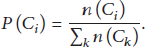
Baseline Model 1 (BM1). In this baseline, we have considered the most frequent check-in category in the training data. Let 
Baseline Model 2 (BM2). Markov models are built for predicting the next place of visit based on the latest visited location, say, 
Here, we want to mention that, in Section 2.4, we form Markov models (MMs) considering amount of time between consecutive visits. Therefore, if we use this baseline model to predict future place, we have only one transition matrix, but in MMs, we have different transition matrix depending upon the granularity of time.
Baseline Model 3 (BM3). As described in Section 2.3, we discuss the need of different window size for each category while predicting the future place of visit. This baseline is defined to show the importance of our approach for deriving window size for each category. For this, we use fixed window size for each category and show the performance against our approach used in Algorithm 1. Similar to BBC in Section 2.3, in this baseline, Naive Bayes is used as binary classifier
3.3. Results
We conduct two sets of experiments. In the first set, we compare the performance of model BBC proposed in Section 2.3 with Baseline Model 3 (BM3). In the second set of experiments, we compare the performances of proposed models with Baseline Models 1 and 2.
3.3.1.
versus BM3
The objective of this set of experiments is to show that BBC performs better when feature vectors are constructed by using window sizes derived by Algorithm 1 for training and testing. We want to recall that window size derived for category
For this, first we show the performance of the classifier on same window size for each category (BM3). One by one, we use five different window sizes that are 5, 10, 20, 30, and 100 hours. Results are shown in Figure 2. WinN represents the performance of BM3 when window size of past tweets is set to N hours. From these results, we observe that BM3 performs better when the size of a window is 10 hours for each category. Also, BM3 performs similarly on both test sets, that is, seen (TS1) and unseen (TS2), which validates that this classifier can be applied to wide variety of users. These results also support our hypothesis that words in tweets posted by users are highly correlated with the future activity or the location of that activity done by that user. By learning the relation of words and locations, BM3 infers the future location using words with high accuracy.

Performance of BM3 on different window sizes for top 5 accuracies. WinN represent the window size of N hours, where
Results shown in Figure 2 validate the existence of the relationship between words and future location. By observing the text in a window, we found out that using same window (BM3) for all categories does not model the problem appropriately. If the window size is 5 hours then the words are very few which results in erroneous predictions. But if we increase the window size, then some words may come which have no role in predicting the current location. For example, tweet like “now looking for some fun” tweeted 30 hours before has no significance in deciding the current activity. From the above results, we found optimum window size is 10 hours for BM3.
For appropriate modeling, as discussed in Section 2.2, we derive window size for each category by using Algorithm 1 for training and testing. We compare these two approaches that are BM3 (10 hours) and
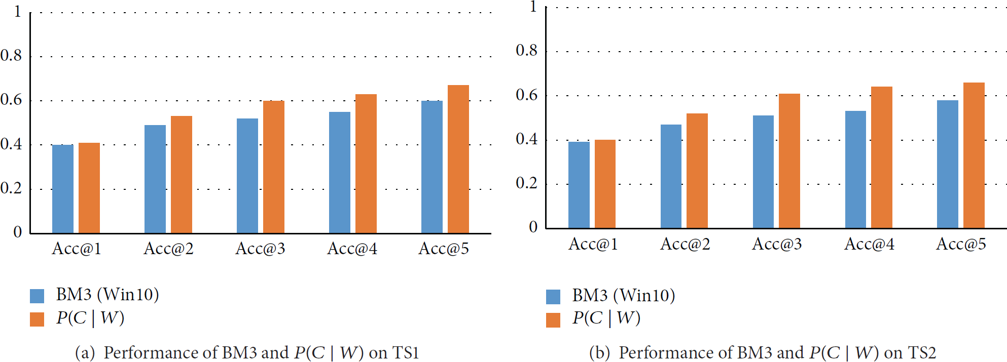
Performance of BM3 and
3.3.2. Comparison of Proposed Models with BM1 and BM2
In this section, we compare the proposed models with BM1 and BM2. The performance of our proposed models outperforms both baselines as shown in Figure 4. We can see that MMs perform much better than BM2. The reason of this improvement is that when we use BM2 only, we have only one transition matrix with no time information in it. Thus, the only input to BM2 is previous visited category. But when we use MMs for prediction, we have two input parameters that are previous visited category and the time duration when it is visited. Based on the time duration we pick the corresponding transition matrix for computing predictions. The information of visiting preference according to time is lost in BM2, hence resulting in erroneous predictions.

Comparison of proposed models with baselines.
4. Related Work
In last decade, researchers have used Twitter data for predicting various things in future. Bollen et al. [2] used tweets for predicting stock market index with high accuracy. Similarly Asur and Huberman [3] predict box-office revenues of movies in advance using related tweets.
Tweets are also explored heavily for inferring users interests for commercial purposes. References [4–6] have used different techniques over tweets for inferring user interest and show that tweets contain a lot of valuable information related to user interest.
For recommendation also people used Twitter data. For example, Sadilek et al. [7] used tweets to recommend those restaurants that user should not go. References [8–10] proposed a recommender system for news recommendations by modeling the user profile and exploiting the tweet-news relationship.
With the exponential growth in usage of smart phones, now users publish millions of tweets frequently from anywhere and at any time. Because of this, one other field emerged that studies the mobility prediction of users; that is, where the user will be? or where he was when given tweets were published? References [11–13] have shown that by using Twitter data we can predict the location of user with high accuracy. But the granularity level of predicting the user location using tweets is at either the country level or regional level. For example, Han et al. [14] predict user location, that is, country or region by identifying location indicative words (i.e., frequent word used at the specific location), in contrast to our approach where we predict locations such as shop, church, and restaurant, where granularity level is very deep.
Some of the efforts have been made for predicting user location such as restaurant and shops, but the data used there are generated by Location Based Social Networks (LBSN). Using LBSN for prediction is very different from using Twitter, as Twitter data is very unstructured and challenging in comparison to structured data of LBSN. References [15–19] have explored LBSN (Foursquare) for recommending or predicting next location to the user.
Some people used text published by users for deriving personality traits and based on common traits recommendations have been made. For deriving personality traits Linguist Inquiry and Word Count (LIWC) [20] had been used frequently. References [20–29] have shown that lexicons used by people can be used for understanding their personal values and how to use these traits for a recommendation. Though all these approaches have been used extensively in analyzing personality traits, these also have shortcomings of predefined word category correlation. Alternatively, Schwartz et al. [30] used rather different approach for using vocabulary known as open-vocabulary technique (using all set of words available on social media) in comparison to closed-vocabulary technique, Linguistic Inquiry and Word Count (LIWC) [20], where some predefined sets of words are used for deriving the personality traits. In their study, they have shown that by using the open-vocabulary approach they got higher state-of-the-art accuracy in predicting gender in comparison to LIWC by exploring latent factors that are not captured by closed-vocabulary approach. Motivated by this approach, we have used all words available on timelines for modeling the users' behavior.
5. Conclusion
In the present work, we study the problem of predicting next place of visit using tweets. We proposed a methodology for predicting next place of visit for user. For experiments, we crawled more than 4600 users' timelines from Twitter. For modeling and generating ground truths, we labeled those tweets with visited locations where relevant information is present. For labeling tweets, we propose simple pattern matching technique labeling tweets with high accuracy. We have also proposed an algorithm for deriving optimal length of window for each category for deriving feature vectors which is used in training and testing of BBC (bank of binary classifiers). From this trained model, BBC (Naive Bayes), we compute the probabilities of visiting next place. To account for the time of last places visited, we trained Markov models that also compute probabilities of visiting next places. Assuming the independence of probabilities produced by bank of binary classifiers and Markov models, we combined these two probabilities. From experiments, we found out that probabilities of visiting next place increased up to 80% from 65%. This shows that our model can be potentially used in location based advertising, intelligent resource allocation, and so forth. Also, similar performance of proposed model on both seen and unseen data sets make it applicable to wide variety of users.
Footnotes
Conflict of Interests
The authors declare that there is no conflict of interests regarding the publication of this paper.