
Abstract
Sensor nodes in wireless sensor networks are deployed to observe the surroundings for some phenomenon of interest. The fundamental issue in observing such environments is the area coverage which reflects how well the region is monitored. The nonuniform sensor nodes distribution in a certain region caused by random deployment might lead to coverage holes/gaps in the network. One of the solutions to improve area coverage after initial deployment is by sensor nodes mobility. However, the main challenge in this approach is how to increase area coverage with the least energy consumption. This research work aims to improve area coverage with minimal energy consumption and faster convergence rate. The Edge Based Centroid (EBC) algorithm is presented to improve the area coverage with faster convergence rate in a distributed network. The simulation based performance evaluations of the proposed algorithms are carried out in terms of area coverage, convergence rate, and energy efficiency. Compared to the existing works, EBC improved area coverage with faster convergence. It is concluded that the proposed algorithm has improved area coverage with faster convergence and minimal energy consumption.
1. Introduction
Wireless sensor networks (WSNs) have gained considerable worldwide attention in different research communities in recent years, due to their widespread applications in many scenarios. Such applications include battlefield surveillance, forest fire detection, disaster monitoring, and postdisaster operations [1–4]. They significantly improve the capabilities to control and monitor the physical environment. The utilization of sensor networks is transforming the traditional techniques of collecting data, linking the gap between physical and virtual world [5, 6]. In WSNs, sensor nodes can be deployed randomly or deterministically; however, they should be appropriately placed to achieve sufficient area coverage level for better monitoring of sensing field [7–9].
Although the deterministic deployment is applicable in some application, there are some working environments that are related to natural disaster areas, harsh environments, and toxic regions in which sensor deployment cannot be deterministically or manually deployed. Deploying sensor nodes with the aid of an aircraft or similar vehicles randomly is one of the possible ways in such environments. However, using this technique (random deployment), the initial landing positions of sensors cannot be uniform or controlled, due to the existence of obstacles such as buildings, trees, and wind, causing some areas of the sensing field (SF) to be more dense than others [10]. Thus, the sensor nodes may not adequately cover the SF, and the highly dense area will cause the sensor network to be an unusual or abnormal network [11, 12]. Therefore, it is essential to make use of mobile sensors, which can move iteratively to a better location that can give the required coverage.
The main goal of mobile sensor network is to improve the area coverage [13]. To achieve this goal, a group of sensors have to be relocated and deployed in more suitable locations in order to monitor the SF effectively. Mainly, WSNs in terms of mobility control are of two types: centralized and distributed. In centralized WSNs, sensors are controlled by a sink node or a central server. However, in the distributed networks, sensors are self-controlled.
Due to the nature of distributed networks that is more appealing to minimize the information exchange between the sensor nodes, no sensor has a priori information of the SF and initial positions of other sensors [14]. In addition, each sensor node has limited sensing and communication abilities which make the sensor nodes unable to obtain the entire network information [15, 16]. Therefore, sensors are deployed randomly and allowed to move and communicate with their neighbours by exchanging information related to each of them. The advantage of this kind of deployment is that sensors can be deployed and work in environments that are harsh or not easily accessible. Commonly, the SF is partitioned into small convex polygons named Voronoi [17–19], such that each polygon will contain only a single sensor node that only needs to cover its own polygon.
In this paper, a distributed movement assisted sensor deployment algorithm, the Edge Based Centroid (EBC), is proposed to enhance area coverage in a distributed mobile sensor network which can be valuable in terms of area coverage. The EBC algorithm tends to move sensor nodes towards the centroid of local Voronoi polygon, from their initial deployment position. The sensor nodes movement is iterative; this is one of the proposed algorithm's main features, in addition to the certainty of coverage increment or stability after every iteration.
The rest of this paper is organized as follows. Section 2 presents some of the related works. Section 3 describes the proposed distributed algorithm of mobile sensors. Section 4 presents the proposed EBC method. Section 5 shows the simulation results and discussion. Lastly, Section 6 is the conclusion of the paper.
2. Related Works
Recently, there exist significant works on sensor deployment and coverage related issues which have kept the area as an active research domain. Directed coverage is used to monitor the area in between two boundaries by a sensor network [20]. The appropriate location to place sensors nodes is vital [21], in monitoring smaller or larger region [22]. Sufficient coverage is essential to WSN [23], while the improvement of coverage is important after the initial deployment of sensor nodes. The distributed movement strategy is commonly used to improve the area coverage of MF by moving the sensor nodes from one location to another [24, 25]. The initial locations of deployed sensor nodes, and where to relocate them, are vital to network coverage [14]. In most of the distributed movement algorithms, monitoring field (MF) is partitioned into subareas, with different sensor node assigned to a particular location. These partitioned subareas cover the entire MF; if the sensor node assigned to monitor a particular subarea cannot detect any expected event within its subarea, no other sensor node can detect it [26]. Therefore, examination of each subarea for coverage hole and calculation of new candidate location is the responsibility of deployed sensor node in that subarea. When a sensor node is unable to cover its own subarea, then there exists a coverage hole (uncovered area).
The challenge before many current distributed movement assisted algorithms is the calculation of a new candidate location within its subarea which is not considered before relocating sensor node [27]. This has constituted a main concern to researchers for coming up with solutions that will address such problem in mobile wireless sensor network [24, 28]. In spite of calculating the new candidate location in its subarea that will enhance area coverage, many of the earlier and some current works proposed algorithms that were unable to cover their subarea adequately. However, a network with coverage holes will not be able to satisfactorily carry out its monitoring task. On the other hand, most of the distributed movement algorithms were designed to have much iteration in their local region before determining the new position. At the end of iterations, this leads to higher energy consumption incurred by sensor nodes movements.
To address those issues of sensor node relocation to a new candidate location that will enhance the area coverage, various approaches have been proposed [28, 29]. Wang et al. (2006) proposed three different distributed movement assisted sensor deployment algorithms, VEC, VOR, and Minimax, to improve the total area coverage. Voronoi diagram is used to partition the MF into n convex polygons where every polygon enclosed one sensor node only. The methods use their local polygon information to calculate the new candidate location to move sensor node. In comparison with other techniques, the VEC approach uses virtual force between two sensor nodes to push them away from each other at a certain distance. Minimax and VOR algorithms are greedy, which try to fix the largest coverage hole by moving sensor node towards the farthest polygon vertex. The sensor node close to a narrow edge of its polygon did not require it to move towards the farthest vertex. The result of such movement may not reduce coverage hole, but rather it can increased in some cases. The two vertex base methods, Minimax and VOR algorithms, are designed to move towards the farthest Voronoi polygon vertex to reduce coverage hole. But in some cases moving towards the farthest vertex with the aim of decreasing the distance may not always reduce the coverage hole, because some polygons may have a narrow shape. To further address the stated problem, four local movement methods are proposed in [24]. The calculation of new candidate locations in those algorithms is by considering circles whose centre is positioned within their respective polygons. There are some cases (rounds) in which the centroid of those circles is outside the polygons, meaning that there is no movement in that round by the affected sensor nodes. This problem makes the algorithms have more rounds before the algorithm converges. The more the rounds it takes, the more the sensor resources are being consumed; examples of resources include energy since sensors have to communicate before constructing their local polygon. Therefore, the proposed EBC distributed movement assisted algorithm addresses the highlighted problems in existing works discussed, which serves as the main differences between the proposed and current work.
3. Preliminaries
3.1. Sensing Models
The sensing model describes the possibility of event detection by sensor in monitoring field [30]. Every sensor type has its own unique sensing model which is characterized by its sensing area, accuracy, and resolution. The sensing area relies on numerous factors such as the signal strength generated from the source, distance between the sensor node and source, the rate of attenuation in propagation, and the required self-confidence sensing level [30]. In [31], a network of acoustic sensors is deployed to detect mobile vehicles. The sensor nearer to a vehicle can detect higher acoustic signal strength than the one farther away from the vehicle due to signal attenuation, and as a result there is higher confidence of detecting vehicles [31]. In this study, isotropic sensing model is considered, which means identical sensing ability in all directions [32]. Each sensing area is associated with a sensor node that is represented by a circle with the same radius. When comparing sensing coverage algorithms, this is a common assumption as in [7, 33, 34].
3.2. Voronoi Diagram
The Voronoi diagram is a basic method of partitioning an area [19]. It is one of the important computational geometry tools for resolving coverage problem of WSNs [35, 36]. The Voronoi diagram of a collection of points partitions a given place into several polygons, which represents the proximity information about a set of geometric nodes; Figure 1 is an example of Voronoi diagram. Every point in a given polygon is closer to the node in that polygon than to any other node in the plane, which is known as generating point [37]. Let us consider a given set of network sensors by
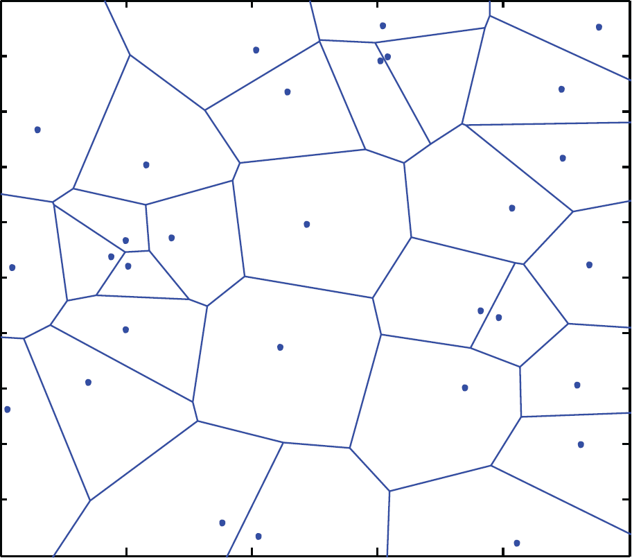
Voronoi diagram.
4. Edge Based Centroid Algorithm
In this section, detailed description of EBC algorithm is given; it includes how to carry out the collection of location information, calculation of new candidate location, sensor node relocation, and algorithm termination. The proposed method is based on Voronoi diagram that represents the nearest information about a set of sensors. Sensing and detection of an expected event in a local polygon are the responsibility of each sensor. The sensor nodes use iterative movement for relocation from one location to another in this algorithm. This is the main feature used by this method until the termination condition is fully satisfied.
4.1. Characteristics of the Network
Before going into the method of sensor deployment, it is important to highlight different assumptions of the sensor networks. The following network features are assumed:
The sensing field is a flat surface without any obstacle. All the sensor nodes are homogeneous and autonomous with the ability to locate themselves in the sensing field.
Communication topology is connected as in [38], so that sensor location information about other sensors can be obtained through appropriate communication routes. This will enable accurate calculation of its polygon.
4.2. Location Information Collection
In the first place, every sensor node
4.3. Calculation of New Candidate Location
To calculate the new candidate position in a local polygon, each sensor node will now check its local polygon for any possible coverage holes. If there exists any coverage hole, the sensor node finds a new candidate location for itself by using EBC method, so by relocating there it will eliminate or reduce the size of the coverage hole. The local coverage of local Voronoi polygon is calculated by the intersection of the polygon and the sensing circle. To determine the existence of local coverage hole (LCH) in each polygon, three possible cases of LCH occurrence are considered:
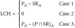
Case 1 (
).
Sensing range is fully included inside polygon as shown in Figure 2: coverage hole = polygon area (
Figure 2 illustrates the case in which the entire sensing range is covered by the polygon. In this case, it can be seen that some area of the polygon is uncovered which gives a coverage hole in that region. So the area of the polygon and sensing range inside the polygon will be calculated, and then the area of the sensing range is subtracted from the area of polygon.
Sensing range fully inside polygon.
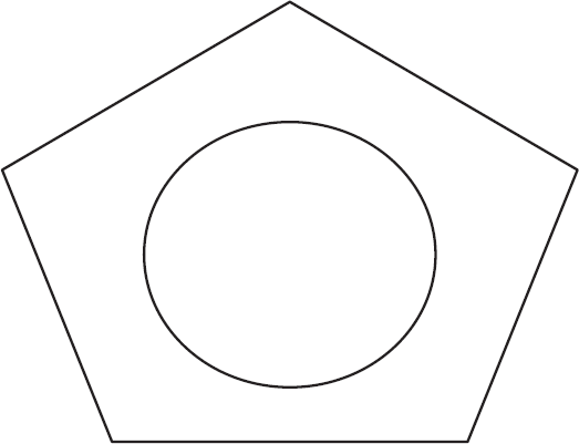
Case 2 (coverage hole = 0).
Polygon is fully covered by the sensing range as illustrated in Figure 3: coverage hole = 0.

Sensing range fully covered the polygon.
Case 3 (
).
Polygon is partially covered by the sensing range, meaning that there is an intersection between sensor node sensing range and the polygon as shown in Figure 4: coverage hole = polygon area (

Intersection between polygon and sensing range.
Figure 4 is an illustration of the case in which sensing range and the polygons are intersecting each other. So, due to that, intersection of some part of the polygon is covered by the sensing range while another part is not covered resulting in a coverage hole. However, due to the fact that we have to calculate the exact covered area from the polygon and the uncovered region which is the coverage hole too, we start by calculating area of polygon and then subtract the covered area from it; this will give the local coverage hole (LCH) of that polygon as given in

The covered polygon area by sensing range has to be calculated by subtracting it from the total polygon area. In the intersection region, a new polygon will be constructed from the big polygon to enable us to calculate the exact covered area. In constructing it, some segments may be created pending on the polygon type and sensing range area that is inside the polygon. Equation (3) represents how the covered area is being calculated:

Algorithm 1 calculates polygon and sensing range intersection in each local polygon so as to determine covered and uncovered areas, so a new candidate location to relocate the sensor node can be calculated.
(1) Find the intersection point between polygon and sensing range (2) Construct a new polygon based on the old polygon vertices that are located inside the SR and the intersection points (3) Find the area of the new constructed polygon (4) Find the area of circle segments located inside the polygon (if any)
4.3.1. Calculating New Candidate Location with EBC Algorithm
The EBC algorithm fixes coverage hole by relocating sensor node to the centroid of the polygon as shown in Figure 5. In finding the candidate location, each sensor calculates the length of all edges of the polygon (

EBC sensor deployment.
4.3.2. Polygon Edge Midpoints Calculation
To find the exact midpoint (MP) of polygon edges

4.3.3. Total Coverage of Monitoring Field Calculation
The total area coverage of the monitoring field is after calculating the local coverage of each Voronoi polygon in the sensing field of the partitioned monitoring field. The total coverage of the entire field is presented in

Step 1. For each Step 2. Repeat Step 3. For each Edge Step 4. Find the Mid-Point (MP) of Edge Step 5. Record the MP end for Edge Step 6. Consider a new polygon where the recorded MPs as Vertices Step 7. Stop when vertices are very close to each other Step 8. Considered the Candidate position as the statistical average of the vertices Loop to next polygon
4.4. Sensor Node Relocation
When the new candidate location has been calculated, with respect to the new location obtained for sensor node to relocate, the current location will be compared to the new location if there is an increase in area coverage of the sensor node that moved or else maintained its current position. Figure 6 shows the current location of the deployed sensor node and the new candidate location to be moved if the covered area of new candidate location is greater than the current local covered area. The current location is the initial deployment position of sensor node. The previous location of each sensor node is always recorded in order to avoid or control oscillation. The moving oscillation may occur when a new hole is generated due to the sensor node leaving its current location. Sensor nodes are not allowed to go back to their previous location as a control measure. Before a sensor node moves, we first check and compare the newly calculated candidate position with the previous position from the recorded position history. If the new candidate position is the same as the previous candidate position, then the sensor will not move and it will maintain the current position, and direction of movement is opposite to the previous one.

Current and new candidate location.
4.5. Termination of Algorithm
In this section, we have the criteria for terminating the program iteration. In this research work, two termination criteria are considered. Firstly, if there is no increment in the local area covered by sensor nodes in its local polygon with 1% or more. The increment is relative to the previous local coverage; always the current calculated area coverage will be compared with the previous one to ascertain the increment. Secondly, if n number of iterations is reached, which is
Input: MFL = integer // Length of Monitoring field Sensors = integer // Number of Sensor nodes deployed MR = integer // Maximum number of rounds Srange = integer // Sensing range radius Scom = integer // Sensor communication range PermeterEnergy = 8.268 // Energy consumed per 1 meter Variables Positions = [ ] // Array variable of size (Sensors, 2) to record the positions totalcov = 0 // To record the calculated coverage totalcovpercent = 0 // To record the calculated coverage percentage Round = 1 // T count number of rounds totalEnergyCons = 0 //To Record total energy consumed VD = [ ] // Array to save voronoi diagram Start (1) newpositions = [ , ] // Array of new positions (2) Positions = rand (sensors, 2) // Generating random initial positions (3) VD = Voronoi (positions) // Voronoi generation with the generated position (4) totalcov = CalculateCoverage (VD, positions) // Function to calculate total coverage (5) totalcovpercent = (totalcov/MFL2) ∗ 100 // calculating total coverage percentage (6) For each polygon in VD (7) Repeat (8) Newpolygon = [ , ] (9) For each Edge in polygon (10) Find midpoint of Edge (11) Append midpoint to new polygon (12) End For each Edge (13) Until vertices are very close to each other (14) (15) (16) (17) (18) (19) (20) IF Round ≤ MR (21) calcEnergy (positions, newposition, permeterEnergy) (22) position = newpositions (23) totalcov = newtotalcov (24) totalcovpercent = newtotalcovpercent (25) else (26) exit Loop (27) End IF Round (28) Else (29) Exit Loop (30) End IF coverage (31) Next Round (32) calculatecoverage average for all rounds (33) calculateEnergy consumption average for all rounds (34) calculateconvergence average for all rounds
5. Simulation and Results
In this section, we present the simulation result. The implementation of the proposed method is carried out in Matlab (version R2011b), on a flat surface without any obstacle of dimension 50 m × 50 m. The total number of sensors (n) deployed randomly varies between
The proposed EBC algorithm is compared with Maxmin-Vertex, Maxmin-Edge, Minmax-Edge, Minimax, VOR, and centroid algorithms in which common features among them are used in calculating sensor node new candidate location. Three different criteria are used to evaluate the performance of the EBC method against other existing algorithms under the same distributed networks system such as sensors deployment quality, energy consumption, and network convergence rate.
5.1. Sensors Deployment Quality
The deployment quality of sensor network is the area coverage by deployed sensor nodes. Sensor nodes relocate from one location to another in order to enhance their area coverage. The coverage is calculated in two steps: each sensor first calculates its local Voronoi polygon coverage, then followed by the summation of all the calculated local coverage values in the monitoring field. Figure 7 shows the coverage percentage of the proposed method and other existing methods. The final results obtained are the average values of 100 runs of each algorithm with different initial random deployment. This reveals that coverage of the sensing field increases as the number of sensor nodes increases. Comparing EBC algorithm and other existing methods, VEDGE, Maxmin-Vertex, Maxmin-Edge, Minmax-Edge, Minimax, and VOR, the results reveal that EBC has higher area coverage rising from 76% with 20 sensors to 98% with 50 sensors as shown in Figure 7. The results reveal that all the methods perform very well with the total area coverage of above 90%. Finally, the results reveal that the proposed EBC algorithm outperforms existing methods when compared in terms of area coverage. This is due to the fact that the algorithms always ensure that the new candidate location to be moved is greater than the current location.

Area coverage percentage.
5.2. Energy Consumption
The energy consumption is defined based on a sensor node local movement to a certain distance in order to minimize or eliminate a coverage hole. The movement energy consumed in the proposed EBC algorithm and existing methods is measured or calculated to determine how energy has been consumed by each of the algorithms. The consumed energy in relocating a sensor node to n meters is in two parts as in [29]: starting/braking energy and moving distance energy. For braking or stopping, the energy needed to overcome the static friction in order to move it again is also the same as the energy value to move 1 m distance as in [42]. The moving distance can be calculated as cumulative energy for the algorithm to complete the 30 rounds or the energy consumed per round. We considered the cumulative energy consumed for 30 rounds. The final cumulative consumed energy results obtained are the average values of 100 runs of each algorithm with different initial random deployment as shown in Figure 8. The results show that moving more sensor nodes or covering far distance by few sensor nodes can lead to higher energy consumption. Comparing the proposed EBC algorithm with current works, the results reveal that EBC has lower energy consumption in three scenarios ranging from 708 joules to 888 joules, except in one scenario (last scenario with 50 sensor nodes) of VOR method with 627 joules and EBC with 708 joules. The low energy consumption recorded by VOR algorithm in that scenario is due to lower area coverage of 95% achieved compared to EBC with 98%, which reveals that there is more sensor movement in EBC to achieve that coverage than VOR. The presented result in Figure 8 finally reveals that EBC algorithm outperformed the existing methods in terms of energy consumption. This is because the distance travelled by most of the sensor nodes to their new candidate location is not much, and movement takes place only if there is an increment in the area coverage.

Cumulative energy consumption.
5.3. Convergence Rate
The convergence rate is presented as the number of rounds in which a method reaches a stage in which there is no increment in area coverage based on a certain threshold value. To determine the convergence rate, we calculate the total area coverage of the covered area at each round and checked whether the area coverage increased with a threshold value of 1% or more and then we move to the next round; otherwise, the algorithm stopped at that round. Then, the number of rounds to reach convergence is recorded. Comparing the proposed EBC algorithm with existing works, the results in Figure 9 reveal that EBC algorithm has the lowest convergence rate ranging from two rounds to four rounds. This happened due to the fact that the area coverage increment in each round in EBC algorithm is less than the threshold value (1%).
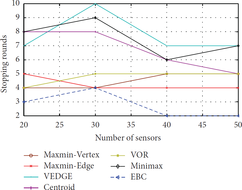
Convergence rate.
6. Conclusion and Future Work
This paper proposed Edge Based Centroid (EBC) algorithm that enhanced area coverage of monitoring field with minimal energy consumption in a mobile sensor network iteratively. The proposed EBC algorithm is based on Voronoi diagram that partitions the sensing field into polygons with one sensor node each to monitor any event in its respective subregion. The mobile sensors are moved to new calculated candidate location that is at the center position of each polygon from its current or initial location, which improves area coverage as shown by the results. Using this algorithm for sensor nodes relocation, a set of rules were applied to ensure that the center of each polygon is calculated before moving the nodes. In terms of movement energy consumption by sensor nodes, the simulation results reveal improved performance of the proposed EBC algorithm in different scenarios.
Considering the scope of this paper which is based on distributed network, real data delivery model is not considered. In future work, the performance of EBC algorithm will be analyzed in a centralized solution that has a sink node. The practical implementation of the proposed EBC algorithm on real hardware devices is needed so as to observe the real behavior of the algorithm. We aim to develop a small test bed for practical implementation of the proposed algorithm on real hardware devices and evaluate its results.
Footnotes
Competing Interests
The authors declare that they have no competing interests.
Acknowledgments
The authors would like to extend their sincere appreciation to the Deanship of Scientific Research at King Saud University for funding this research. The research is supported by Ministry of Education Malaysia (MOE) and conducted in collaboration with Research Management Center (RMC) at Universiti Teknologi Malaysia (UTM) under VOT no. R.J130000.7828.4F708.