Sage Journals: Discover world-class research

Abstract

Urban road travel time is an important parameter to reflect the traffic flow state. Besides, it is one of the important parameters for the traffic management department to formulate guidance measures, provide traffic information service, and improve the efficiency of the detectors group. Therefore, it is crucial to improve the forecast accuracy of travel time in traffic management practice. Based on the analysis of the change-point and the ARIMA model, this paper constructs a model for the massive data collected by loop detectors to forecast travel time parameters. Firstly, the preprocessing algorithm for the data of loop detectors is given, and the calculating model of the travel time is studied. Secondly, a change-point detection algorithm is designed to classify the sequence of large number of travel time data items into several patterns. Then, this paper establishes a forecast model to forecast travel time in different patterns using the improved ARIMA model. At last, the model is verified by simulation and the verification results of several groups of examples show that the model has high accuracy and practicality.

1. Introduction

The travel time (TT) refers to the average time of all vehicles to pass a section of a road, as is shown in Figure 1. If $T_{i j}$ means the time that vehicle $i (i = 1,2, \dots, m)$ travels from detector $l_{j}$ to detector $l_{j + 1}$ $(j = 1,2, \dots, n - 1)$ , then the travel time of section $[l_{1}, l_{n}]$ can be defined as $T T_{i} = \sum_{i = 1}^{m} (\sum_{j = 1}^{n - 1} T_{i j}) / m$ .

Figure 1

Distribution of the loops on the road.

Urban road travel time is an important parameter to reflect the state of traffic flow of a road [1, 2]. Based on the forecast information of travel time, the traveler can choose their travel route reasonably [3], and the traffic management department can establish impeccable guiding measures [4]. Thus, the precise forecast of travel time plays important role in improving the quality of urban traffic information service and the efficiency of detector group on the road [5], which has drawn great attention from scholars all the time.

Mori et al. give a thorough classification of the methods for travel time forecasting and they divide the forecasting model into naive model, traffic flow model, data model, and hybrid model [6]. Vlahogianni et al. give a short-term traffic forecasting method of where we are and where we are going [7]. Shao et al. give the method of real-time travel time forecasting based on the improved Kalman filter [8]. Chilukuri et al. forecast the short travel time of the highway by using microsimulation technique [9]. Yao and Zhang give the short-term forecasting algorithm of interval travel time for urban freeway by analyzing the floating car data, which provides the basis for the subsection forecast of the travel time [10]. Zhao et al. propose a forecasting algorithm based on equal interval interpolation and Sage-Husa adaptive Kalman filtering, which effectively improve the forecast accuracy of travel time [11]. Gui and Yu come up with a new idea for travel time forecast by establishing a forecast model with the selective forgetting ability, which enables the algorithm to adapt to trip conditions changes well [12].

The literatures which have been mentioned above provide some idea for this paper to forecast the travel time based on massive data collected from loop detectors. First, travel time and the traffic state of the road have a certain correlation. Besides, most of the travel time forecast models are using historical data for analysis. And the characteristics of traffic flow tend to change with the seasons and the environment in certain regularity. Thus, if the traffic flow can be divided into several state intervals, this means that the different intervals in the same pattern have the similar statistical characteristics of the mean and variance. As a result, it is easier to get the more optimized forecast result than to obtain it by using the global search.

Therefore, this paper proposes a travel time forecasting model based on change-point detection, which uses the change-point detection to identify different patterns of travel time series and set up the forecasting model by ARIMA in each of the patterns.

The rest of the content of this paper is summarized as follows: (1)

Preprocessing of the massive data collected by the loop detectors and calculation of travel time parameter.

(2)

The pattern partition of travel time series based on change-point analysis and setting up the forecasting model based on ARIMA.

(3)

Verification of the travel time forecasting model based on actual data.

2. Identification and Correction of the Loop Detector's Data

Because of the reasons such as the detector fault, the fault of communication system, and the environmental factor, the real-time detector data contain some unpredictable data missing or invalid data. Therefore, it is necessary to preprocess the data collected by the traffic detectors [13]. So this paper gives the basic rules to identify and correct loop detector's data based on practical experience.

Basic Rule 1. When the data of traffic volume, speed, and occupancy rate is negative or null, it is recorded as the error data. When the data of volume is significantly greater compared to the maximum volume of road ( $Q_{m a x} = f_{c} C T / 60$ ), it is recoded as the error data. When the data of speed is significantly greater compared to the maximum allowable speed or capacity of the urban road, it is recorded as the error data. When the data of occupancy rate is not less than 100%, it is recorded as error data.

Basic Rule 2. When the data of occupancy rate is greater than some reasonable threshold such as 95% and the data of speed is greater than the normal range such as 5 km/h, it is recorded as the error data. When the speed is zero and the volume is not zero, the data is the error data. When the volume is zero and the occupancy rate is not zero, the data is the error data. When the average effective vehicle length ( $AEVL (m) = (10 \times v \times h) / q$ , v: speed $〈km/h〉$ ; h: occupancy rate $〈%〉$ ; and q: volume $〈vehicle volume / {(lane/hour)}^{- 1}〉$ ), is beyond reasonable limits (such as $AEVL \in [1.5 m, 30 m]$ ), it is the error data.

Basic Rule 3. Each data item should be recorded similarly by n piece of data in time t before it. And the data should be done in first-order difference. If the difference value of first-order does not belong to the reasonable change range made by n data before it, this data can be defined as the abruptly changing distortion data.

The data collected by the detectors can be expressed as four-tuple structure, that is $[t, q, v, h]$ . Based on the basic rules which have been discussed above, this paper proposes an algorithm to accomplish the real-time identification and correction of loop detector's data.

Algorithm 1.

Step 1. It is determining $Q_{m a x}$ , $V_{m a x}$ , and $H_{m a x}$ according to the actual situation of the detectors on the road. Test all of the data; if $q > Q_{m a x}$ or $v > V_{m a x}$ or $h > H_{m a x}$ , the data will be defined as error data.

Step 2. When the occupancy rate $h > H_{1}$ $(H_{1} = 95 %)$ and $v > V_{1}$ $(V_{1} = 5 km/h)$ , the data is recorded as the error data.

Step 3. When $v = 0 (km/h)$ and $q \neq 0$ (vehicle number/(lane/hour)⁻¹), the data is the error data.

Step 4. When $q = 0$ (vehicle number/(lane/hour)⁻¹) and $v \neq 0 & & h \neq 0$ , the data will be defined as error data.

Step 5. Calculate the average effective vehicle length (AEVL) according to the current detected data. If $AVEL \notin [1.5,30]$ , exclude this data.

Step 6. It is using the reasonable and nearest data to replace those error data which have been found in Steps 1–5.

Step 7. It is using the first-order differential operation to process data. If the difference value does not belong to the reasonable change range made by the differential mean value and variance of n piece of data before it (such as $[\bar{d} - ε_{0} * σ_{d}, \bar{d} + ε_{0} * σ_{d}]$ ), this data can be defined as the abruptly changing distortion data. Then use $p_{n - 1} + (1 / ε_{0}) * d_{n}$ to replace it.

3. Calculation of Travel Time Based on the Data from Loop Detector

Using the preprocessed data, the travel time parameter values can be calculated [14]. The calculation result of the travel time parameter is usually related to the speed of the vehicle on the road.

Assume the speed is conformed to liner change and the upstream and downstream of each section of the road have a detector and each trip chain has multiple parts, so that $v_{i} (t)$ , speed of the vehicle between detector k and detector $k + 1$ , can be expressed as

\begin{matrix} v_{i} (t) = V (k, d) + \frac{s_{i} (t) - s_{k}}{s_{k + 1} - s_{k}} (V (k + 1, d) - V (k, d)) . \end{matrix}

(1)

$s (t) = \int v (t) d t$ , and this equation is a standard differential equation. Due to differential equations it is very difficult to obtain exact solutions; generally we need to seek an approximation to replace it. So $s (t)$ can be obtained by formula

\begin{matrix} s_{i} (t) = s_{i}^{0} + (\frac{V (k, d) (s_{k + 1} - s_{k})}{V (k + 1, d) - V (k, d)} + s_{k + 1} - s_{k}) \cdot (e^{[(V (k + 1, d) - V (k, d)) / (s_{k + 1} - s_{k})] (t - t_{i}^{0})} - 1) . \end{matrix}

(2)

$s_{k + 1}, s_{k}$ stand for the location of detectors $k + 1$ and k. $V (k, d)$ stands for the speed of detector k in time period d and also is the slope of the vehicle motion curve. $s_{i} (t)$ stands for specific motion trajectories of time period d within road section k. ${s_{i}^{0}, t_{i}^{0}}$ is the initial state of the vehicle entering ${k, d}$ range. If $V (k + 1, d) = V (k, d)$ , formula (2) is

\begin{matrix} s_{i} (t) = s_{i}^{0} + V (k, d) (t - t_{i}^{0}) . \end{matrix}

(3)

According to formulas (1), (2), and (3), the formula for time calculation of the road section based on the vehicle moving track can be divided into two situations: (1)

When the speed is fast, consider the following:

\begin{matrix} s_{i}^{0} + (\frac{V (k, d) (s_{k + 1} - s_{k})}{V (k + 1, d) - V (k, d)} + s_{i}^{0} - s_{k}) \cdot (e^{[(V (k + 1, d) - V (k, d)) / (s_{k + 1} - s_{k})] (t - t_{i}^{0})} - 1) > s_{k + 1}, \\ s_{i}^{*} = s_{i} (t_{i}^{*}) = s_{k + 1} . \end{matrix}

(4)

The approximate result for the travel time of the road section is

\begin{matrix} t_{i}^{*} \approx t_{i}^{0} + \frac{(s_{k + 1} - s_{k})}{V (k + 1, d) - V (k, d)} \ln (\frac{V (k, d) (s_{k + 1} - s_{k}) / (V (k + 1, d) - V (k, d)) + s_{k + 1} - s_{k}}{V (k, d) (s_{k + 1} - s_{k}) / (V (k + 1, d) - V (k, d)) + s_{i}^{0} - s_{k}}) . \end{matrix}

(5)

(2)

When the speed is slow, consider the following:

When $s_{i} (t_{d + 1}) < s_{k + 1}$ , the travel time obtained by formula (2) is

\begin{matrix} t_{i}^{*} = t_{i}^{0} + \frac{s_{k + 1} - s_{i}^{0}}{V (k, d)} . \end{matrix}

(6)

This algorithm based on the method mentioned above can be summarized as follows.

Algorithm 2.

Step 1. Launch vehicles, and select sections ( $K = 1$ ).

Step 2. For vehicle in ${s_{i}^{0}, t_{i}^{0}}$ and ${k, d}$ , use formulas (2), (3), (5), and (6) to calculate ${t_{i}^{*}}$ and ${s_{i}^{*}}$ when it runs out of the area. If $s_{i}^{*} = s_{k + 1}$ , set $k = k + 1$ and move to next section. Otherwise, $t_{i}^{*} = t_{d + 1}$ , set $d = d + 1$ , and move to the next data collection period.

Step 3. If $k \geq m$ , it means that the vehicle has arrived at the destination. Record the departure time and arrival time of the vehicle and then stop. Otherwise go back to Step 2 to recalculate the travel time.

Step 4. Set $i = i + 1$ . The number of $i + 1$ vehicles has continuous headway at ${s_{i + 1}^{0}, t_{i + 1}^{0} + h}$ . If $t_{i + 1}^{0} + h > n$ , stop. That indicates that the calculation of the specified time period has been completed.

This algorithm is firstly assuming the motion trajectory of the vehicle on the road and then through using the location-time curve gets the time at which a vehicle runs out of the detector area to obtain the travel time [15]. This method of travel time estimation through time space motion trajectory has high accuracy. The error between the results of the calculation in [13, 16] and the result of this algorithm is below 6%, which means that this algorithm's result is acceptable.

4. Forecast Model for Short-Term Travel Time Based on ARIMA

4.1. Change-Point Searching

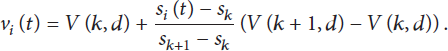
Because the traffic data has different numerical characteristics in different time periods, it can be divided into numbers of similar small states by conditional change-point searching, which can effectively improve the fitting degree of the model. In [17, 18], a new algorithm for state division based on the demand variation of the observation function is introduced. The mean and the variance of the sequence can be expressed by statistical formula.

Whole sequence is

\begin{matrix} {{\bar{x}}_{i}|}_{1}^{n} = \frac{\sum_{i = 1}^{n} x_{i}}{n}, \\ Dev ({x_{i}|}_{1}^{n}) = \sum_{i = 1}^{n} {(x_{i} - {{\bar{x}}_{i}|}_{1}^{n})}^{2} . \end{matrix}

(7)

Convex (concave) wave is

\begin{matrix} {{\bar{x}}_{t}|}_{l_{j - 1}}^{l_{j}} = \frac{(x_{l_{j - 1}} + \dots + x_{l_{j}})}{(l_{j} - l_{j - 1} + 1)}, \\ Dev ({{\bar{x}}_{i}|}_{l_{j - 1}}^{l_{j}}) = \sum_{t = l_{j - 1}}^{l_{j}} {(x_{t} - {{\bar{x}}_{t}|}_{l_{j - 1}}^{l_{j}})}^{2}, \\ j = 2, \dots, k . \end{matrix}

(8)

{l_{j}}

is valley point of peak carve or peak points of the valley curve.

The observation function decides whether to retain the possible change-point. Before that, the control parameter and observation function values of the minimum state variable are required.

Observation function is

\begin{matrix} T (w) = (\frac{B (w, {x_{i}|}_{1}^{n})}{B (w + 1, {x_{i}|}_{1}^{n})}), w = 0,1, \dots, J - 1, \\ B (w, {x_{i}|}_{1}^{n}) = \{\begin{cases} \sum_{g = 0}^{w - 1} Dev ({x_{t}|}_{b^{(g)}}^{b^{(g + 1) - 1}}) + Dev ({x_{t}|}_{b^{(w)}}^{n}), & w = 1, \dots J, \\ Dev ({x_{i}|}_{1}^{n}), & w = 0 . \end{cases} \end{matrix}

(9)

$\{b^{(w)}\}$ is the index set of all J points on the curve and $b^{(0)} = x_{l_{1}} = x_{1}$ .

The algorithm is as follows.

Algorithm 3.

Step 1. Make the travel time series into carve, u represents the time of cycles, w represents the number of change-points, and $e_{e}$ is the auxiliary variable. Set $u = 1$ , $w = 1$ , $e_{e} = 0$ , and $β_{j} = l_{j}$ , $j = 1, \dots, k$ .

Step 2. Select two convex waves along the axis of time from $β_{u}$ on the carve, such as $(β_{u} - β_{u + 1} - β_{u + 2})$ . Then calculate $t^{*}$ :

\begin{matrix} A (β_{u}, β_{u + 1}, β_{u + 2}) = \sum_{t = β_{u}}^{β_{u + 1}} {(x_{t} - {{\bar{x}}_{t}|}_{β_{u}}^{β_{u + 1}})}^{2} + \sum_{t = β_{u + 1} + 1}^{β_{u + 2}} {(x_{t} - {{\bar{x}}_{t}|}_{β_{u + 1} + 1}^{β_{u + 2}})}^{2}, \\ M (β_{u}, t_{1}^{*}, β_{u + 2}) = \max (\sum_{t = β_{u}}^{t} {(x_{t} - {{\bar{x}}_{t}|}_{β_{u}}^{t})}^{2} + \sum_{t = t + 1}^{β_{u + 2}} {(x_{t} - {{\bar{x}}_{t}|}_{t + 1}^{β_{u + 2}})}^{2}), \\ m (β_{u}, t_{2}^{*}, β_{u + 2}) = \min (\sum_{t = β_{u}}^{t} {(x_{t} - {{\bar{x}}_{t}|}_{β_{u}}^{t})}^{2} + \sum_{t = t + 1}^{β_{u + 2}} {(x_{t} - {{\bar{x}}_{t}|}_{t + 1}^{β_{u + 2}})}^{2}) . \end{matrix}

(10)

Step 3. Change-point estimation is

\begin{matrix} R_{u} = \frac{2 A (β_{u}, β_{u + 1}, β_{u + 2})}{(M (β_{u}, t_{1}^{*}, β_{u + 2}) + m (β_{u}, t_{2}^{*}, β_{u + 2}))}, \\ c r_{u} = \frac{M (β_{u}, t_{1}^{*}, β_{u + 2})}{m (β_{u}, t_{2}^{*}, β_{u + 2})} . \end{matrix}

(11)

Consider the following:

(1)

If $M (β_{u}, t_{1}^{*}, β_{u + 2}) \approx m (β_{u}, t_{2}^{*}, β_{u + 2})$ , $1 \leq c r_{u} < 1.3$ , and the sequence change is gently, you do not need to set change-point in $(l_{u}, l_{u + 2})$ .

(2)

If $R_{u} \leq (1 / 4) + 3 / 2 (c r_{u} + 1)$ , regardless of whether $t_{1}^{*} = β_{u + 1}$ , there is $b^{(w)} = β_{u + 1}$ .

(3)

If $1 \geq R_{u} \geq (1 / 4) + 3 / 2 (c r_{u} + 1)$ , seek the nearest peak or valley point of $β_{u + 1}$ and set the left one as $β_{u + 1}^{L}$ and right one as $β_{u + 1}^{R}$ . If $\exists t_{c} \in \{β_{u + 1}^{L}, β_{u + 1}^{R}\}$ have $Dev (β_{u}, t_{c}, β_{u + 2}) = \min (Dev (β_{u}, β_{u + 1}^{L}, β_{u + 2}), Dev (β_{u}, β_{u + 1}^{R}, β_{u + 2}))$ . Then $b^{(w)} = t_{c}$ .

(4)

If $R_{u} > 1$ , then $b^{(w)} = t_{2}^{*}$ .

(5)

Make effective judgments for $b^{(w)}$ offered by (2), (3), and (4); if $T (w - 1) - 1 > ε_{0}$ , keep this change-point; otherwise remove it.

Step 4. If you have $b^{(w)}$ , then $u = u + 1$ , $β_{u} = b^{(w)}$ , $β_{u + 1} = β_{u + 1}$ , $β_{u + 2} = β_{u + 2}$ , $w = w + 1$ , and $e_{e} = 0$ . Otherwise, $e_{e} = 1$ , $β_{u} = β_{u}$ , $β_{u + 1} = β_{u + 1 + e e}$ , and $β_{u + 2 + e e} = β_{u + 2 + e e}$ . When $β_{u + 2} = β_{k}$ , the searching is complete and the algorithm ends. Otherwise go back to Step 2.

The paper [18] has provided a complete method on how to improve this kind of algorithm. However, there has been a crucial control parameter $e_{0}$ for which the algorithm does not give the specific processing formula. That algorithm sets $e_{0}$ as a constant value such as 0.5. In this paper, we will carry out several experiments with different $e_{0}$ , which provide reference to the parameter of travel time inferred from detectors' data.

4.2. ARIMA Forecasting Model

The preprocessing of the time series short-term forecasting model includes stationary test and random test. If the time series is nonstationary, it needs to be transformed into stationary series by differential operation. In this circumstance, the ARIMA model is converted to ARMA model. The sequence of d order differences is expressed as

\begin{matrix} \nabla^{d} x_{t} = \sum_{i = 1}^{d} {(- 1)}^{d} C_{d}^{i} x_{t - i} . \end{matrix}

(12)

ARIMA $(p, d, q)$ model can be expressed as

\begin{matrix} Φ (B) \nabla^{d} x_{t} = Φ_{p} (B) ε_{t}, \\ E (ε_{t}) = 0, \\ V a r (ε_{t}) = σ_{ε}^{2}, \\ E (ε_{t} ε_{s}) = 0, s \neq t, \\ E x_{s} ε_{t} = 0, \forall s < t . \end{matrix}

(13)

The order number p, q of ARIMA $(p, d, q)$ model is based on Autocorrelation Coefficient (ACF) and Partial Autocorrelation Coefficient (PACF) of ARMA after differential operation. And, according to the characteristics of PACF and ACF coefficients, the model identification is carried out.

For random inspection, the data collected by the detector is a large density data point, so the calculation result of travel time is also a large sample of high density, which needs to test the hypothesis by using Q statistics:

\begin{matrix} Q = n \sum_{k = 1}^{m} {\hat{ρ}}_{k}^{2} ~ χ^{2} (m) (m is delay-stage) . \end{matrix}

(14)

When Q is less than the quintile of $χ_{1 - α}^{2} (m)$ , the sequence is pure random sequence. However, when the travel time is modeled by the ARIMA model, if the sample space becomes small, the modified LB statistics can be used:

\begin{matrix} LB = n (n + 2) \sum_{k = 1}^{m} (\frac{{\hat{ρ}}_{k}^{2}}{n - k}) . \end{matrix}

(15)

Because there is only a short-term significant correlation in the sequence, the test for the hypothesis is only for Q and $LB$ with short-term delay-stage, which is generally m less than 10.

After differential operation, the ARIMA model is degraded to the standard ARMA model; its standard form is

\begin{matrix} x_{t} = μ + \frac{Φ_{p} (B)}{Φ_{p} (B)} ε_{t} . \end{matrix}

(16)

In the formula,

\begin{matrix} ε_{t} ~ W N (0, σ_{t}^{2}), \\ Φ_{p} (B) = 1 - θ_{1} B - \dots - θ_{p} B^{p}, \\ Φ_{p} (B) = 1 - φ_{1} B - \dots - φ_{q} B^{q} . \end{matrix}

(17)

There are $p + q + 2$ unknown parameters in ARMA model: $ϕ_{1}, ϕ_{2}, \dots, ϕ_{p}, θ_{1}, θ_{2}, \dots, θ_{q}, μ, σ_{ε}^{2}$ . Matrix estimation is usually used to obtain the value of μ and $σ_{ε}^{2}$ .

Calculate the expectation and variance of formula (16) on each side and get

\begin{matrix} \hat{μ} = E (x) = \bar{x} = \frac{\sum_{1}^{n} x_{i}}{n}, \\ σ_{ε}^{2} = \frac{\sum_{1}^{n} {(x_{i} - \bar{x})}^{2}}{n} = \frac{1 + φ_{1}^{2} + \dots + φ_{p}^{2}}{1 + θ_{1}^{2} + \dots + θ_{p}^{2}} σ_{x}^{2} . \end{matrix}

(18)

The parameters of the equation are reduced to the number of $p + q$ . Least square estimation is used to estimate the parameters of the ARMA model which is obtained by differential operation.

In the case of ARMA $(p, q)$ , the parameter vector is

\begin{matrix} \tilde{β} = {(ϕ_{1}, \dots, ϕ_{p}, θ_{1}, \dots, θ_{q})}^{'}, \\ F_{t} (\tilde{β}) = ϕ_{1} x_{t - 1} + ϕ_{2} x_{t - 2} + \dots + ϕ_{p} x_{t - p} + ε_{t} - θ_{1} ε_{t - 1} - θ_{2} ε_{t - 2} - \dots - θ_{q} ε_{t - q} . \end{matrix}

(19)

Thus, overall observed sum of squared residuals of the sample is

\begin{matrix} Q (\tilde{β}) = \sum_{1}^{n} ε_{t}^{2} = \sum_{1}^{n} {(x_{t} - F_{t} (\tilde{β}))}^{2} . \end{matrix}

(20)

Set the objective function for parameter estimation as $\min Q (\tilde{β})$ and use the weighted least squares method to solve the parameters.

The essence of the weighted least square method is to transform the original data to obtain the new explanatory variables and explained variable. Assume that $x_{i}$ is time series data and ω is the weight of this point, so that weighted least square method is

\begin{matrix} x_{i}^{'} = x_{i} \cdot ω_{i} (x^{'} refers to travel time after transformation) . \end{matrix}

(21)

Then, use (

x_{1}^{'}, \dots, x_{n}^{'}

) to do the least square parameter estimation of ordinary ARIMA model; we can get the optimal parameter vector

{\tilde{β}}^{'}

of the model in weighted transformation. In this way, the formula for the weighted forecast formula is

\begin{matrix} F_{t} ({\tilde{β}}^{'}) = φ_{1}^{'} x_{t - 1} + φ_{2}^{'} x_{t - 2} + \dots + φ_{p}^{'} x_{t - p} + ε_{t} - θ_{1}^{'} ε_{t - 1} - θ_{2}^{'} ε_{t - 2} - \dots - θ_{q}^{'} ε_{t - q} . \end{matrix}

(22)

After removing the weight, the final forecast value is obtained:

\begin{matrix} F_{t} (\tilde{β}) = \frac{F_{t} ({\tilde{β}}^{'})}{ω_{t}} . \end{matrix}

(23)

5. Application Example

5.1. Preprocessing of the Massive Data from Loop Detectors

This paper takes the actual data of 2nd ring road in a big city as an example (detector number is $020^{* *}$ ; line number is Lan 1–Lan 6; date is on Mar. 3rd, 2013; data collection time is 24 hours; sampling interval is 2 minutes; parameters are traffic volume, speed, and occupancy rate; and the total number of data points is 720) to verify the travel time forecasting model based on loop detectors which has been mentioned above. The actual data of Lan 1 is shown in Figure 2.

Figure 2

Data distribution of Lan 1's volume-speed-occupancy rate in 24 hours.

In Figure 2, mutation points can be observed in the data series of all the three parameters. In fact, the data of traffic conditions cannot change more than 500% times within two minutes. So it can be concluded that there are abnormal or distorted data in the actual data and it is necessary to filter those data.

According to Algorithm 1, we can finish the data cleaning. Firstly, according to the definition, the control parameters based on the basic traffic flow principle and the actual physical meaning are set up in Table 1.

Table 1

Selection of filtering model's parameters.

Parameter name	Abbreviation	Experimental values
Section maximum flow	$q_{m a x}$	$q_{m a x}$ = 3600/30
Section maximum speed	$v_{m a x}$	$v_{m a x}$ = 150
Section maximum occupancy rate	$o_{m a x}$	$o_{m a x}$ = 100
Constraints of occupancy rate and speed	$H_{1}$ , $V_{1}$	$H_{1} = 95$ , $V_{1} = 5$

$q :$ volume 〈vehicle volume/(lane/hour)⁻¹ 〉; v: speed 〈km/h〉; and o: occupancy rate $〈%〉$ .

Under the control of parameters listed in Table 1, we can finish the data cleaning to find out the data beyond the maximum control range or contrary to the theory of traffic flow. The result is shown in Figure 3.

Figure 3

Fault data points of filtering intermediate state search.

Use a one-dimensional matrix to record the effectiveness of each record. All the initial value of the matrix is 1. When the abnormal data is detected, the corresponding matrix value is changed into 0. From Figure 3, there is a series of error data points at the time 3:00–6:00, which is consistent with the original graph shown in Figure 4.

Figure 4

Comparison between the actual data and the results of the filter's intermediate state.

Because these error data points do not have actual physical meaning, they are replaced by the closest normal record. After the cleaning, the figure of volume-speed-occupancy rate is shown in Figure 5.

Figure 5

Result of filter's intermediate state.

Data quality has been improved to a certain extent, especially for the speed data. But there still has been mutation in the filtering results. Test the first-order differential of the data to determine the mutation data. The first-order difference graph of intermediate state is shown in Figure 6.

Figure 6

First-order difference graph of intermediate state.

Control parameter of differential operational is $e_{0}$ . Assuming that $e_{0} = 3$ is the parameter of the reasonable change region, if the actual value of the first-order is exceeded three times of the standard deviation control range, change the corresponding position of the effective matrix into 0.

When $e_{0} = 3$ , there are 83 abnormal data points as is shown in Figure 7, which account for 11.5% of the total record. This result is too strict for the data of detectors, so we can increase the value of $e_{0}$ to release the strictness for change range of the data as is shown in Table 2.

Table 2

Result of the filter by different parameters.

$e_{0}$ value	$e_{0} = 3$	$e_{0} = 4$	$e_{0} = 5$
Number of change ranges beyond	83	34	21
Rate of the data beyond	11.5%	4.7%	2.1%

Figure 7

Distortion data distribution when $e_{0} = 3$ .

According to the results shown in the table, $e_{0} = 4$ is more reasonable. Figure 8 is comparison chart between the final result of the filter and the original data, and it can be seen that the algorithm has basically achieved the requirements of the loop detector data's cleaning and preprocessing.

Figure 8

Comparison of the source data and the filter result.

From Figure 3 it can be seen that the algorithm has a small correction for the traffic data and the data with the occupancy rate, but the algorithm has better effect on the speed data. In the process of predicting travel time, the speed of the detector is often used only, which means that the algorithm can be simplified so that it only needs to produce speed data.

Because only the speed data is processed, we need to set the upper and lower limit of speed and the limit of first-order differential change range to restrict data. As a result of using the detector data to calculate and predict travel time, we need three continuous detector's data points to simulate the travel time forecast in whole road network. The sketch map is shown in Figure 9.

Figure 9

Distribution of the three serial detectors on the road.

Under the condition that $e_{0} = 3$ , the filter result of speed after cleaning of the three detectors is as shown in Figures 10, 11, and 12.

Figure 10

Filter result of the speed data of Detector 1.

Figure 11

Filter result of the speed data of Detector 2.

Figure 12

Filter result of the speed data of Detector 3.

As shown in Figures 10~12, the red correction curve basically achieved a reasonable correction of the distortion data.

5.2. Calculation of Travel Time Parameters

Use the travel time conversion model given by formulas (5) and (6); we can do the travel time conversion according to the speed data. For example, when one calculates the travel time driving from east to west, the vehicles pass through sections $\{Detector 1, Detector 2\}$ and $\{Detector 2, Detector 3\}$ . The result is shown in Figure 13 and the unit of time is s/m.

Figure 13

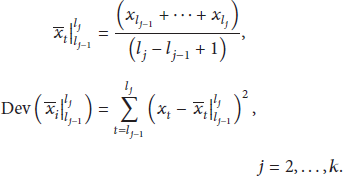
Travel time calculation result from $\{Detector 1, Detector 2\}$ to $\{Detector 2, Detector 3\}$ .

5.3. Pattern Partition of Travel Time Series Based on Change-Point Analysis

Because it is not clear how to choose $e_{0}$ up to the size of the sample, we select 7 values to search the change-point. The result is in Table 3.

Table 3

Result of change-point searching of each section.

$e_{0}$	Searching result of change-point	Number of change-points
0.01	$\{1, 25,59,70,77,90,224,319,326,342,357,376,379,390,393,414,415\}$	17
0.02	$\{1, 25,90,224,375,380,384,390,393,414\}$	10
0.05	$\{1, 225,375,380,390,393,412\}$	7
0.07	$\{1, 225,380,393,412\}$	5
0.1	$\{1, 411\}$	2
0.12	$\{1, 416\}$	2
0.15	$\{1\}$	1

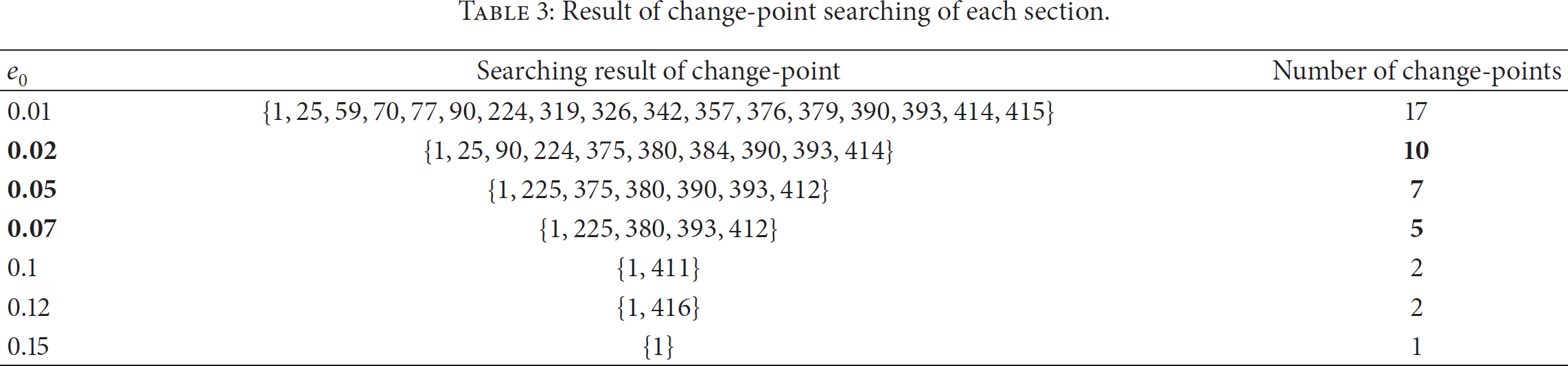
According to the characteristics of the travel time series, we need to select the result that has 5 to 10 change-points. So $e_{0} = 0.07$ , $e_{0} = 0.05$ , and $e_{0} = 0.02$ are all reasonable control parameters. The results of all the reasonable circumstance are shown in Figure 14. We use different colors to indicate different state.

Figure 14

Result of the global state change-point searching.

According to the time sequence diagram, the results of the algorithm are basically completed, and the travel time series is decomposed into a series of time periods with practical meaning.

On the situation of $e_{0} = 0.07$ and $e_{0} = 0.05$ , there are 90 important change-points that were missed. So $e_{0} = 0.02$ and ${1, 25,90,224,375,380,384,390,393,414}$ are ideal controlling parameter and result of change-point control. And the travel time is divided into 9 divisions: 6:00~6:50, 6:50~9:00, 9:00~13:28, 13:28~18:30, 18:30~18:38, 18:38~18:50, 18:50~18:56, 18:56~19:48, and 19:48~23:00.

Then, if we assume that this moment is 17:00, we can predict the travel time of 17:02 and 17:04. The historical data of the forecast model is shown in Figure 15.

Figure 15

Historical data of the forecast model.

5.4. Travel Time Forecasting Based on ARIMA Model

To sum up, we choose ARIMA model to build up the forecast model and regress the parameter. Using the data of 221~330 collected by Detector 1 at the time 13:28~17:00 and testing the time sequence, we found it is a nonrandom stationary sequence. The fix order result of the ARIMA model for the time of 13:28~17:00 is $(2,0, 0)$ .

After the weighted least squares are transformed into ordinary least squares, we use four kinds of weight function to do the fitting experiment and also have the error analysis to the output results. The forecast results of different weight functions are as in Table 4.

Table 4

ARIMA model and forecast result of different weight functions.

Weight functions	Fitting equations	Forecast value on 17:02	Forecast value on 17:04
Square-root	$x_{t}^{'} = 0.000321317 + 0.726226 x_{t - 1}^{'} + 0.191767 x_{t - 2}^{2}$	0.208528	0.206241
Square	$x_{t}^{'} = 0.0000607593 + 0.798534 x_{t - 1}^{'} + 0.204619 x_{t - 2}^{2}$	0.213584	0.215573
Growth rate curve	$x_{t}^{'} = 0.000340756 + 0.717946 x_{t - 1}^{'} + 0.193551 x_{t - 2}^{2}$	0.209668	0.208116
Liner	$x_{t}^{'} = 0.000948595 + 0.617164 x_{t - 1}^{'} + 0.110425 x_{t - 2}^{2}$	0.206278	0.202864

Actual value on 17:02: 0.20577.

Actual value on 17:04: 0.196385.

Error analysis result is shown in Table 5 and we can see that the crucial index MAPE has a certain degree of reduction at the proximal point.

Table 5

Error matrix of different model fittings.

Weight functions	ME	MAE	MAPE	MSE
Square-root (global)	−0.000361064	0.01288	7.10089	0.000279502
Square (global)	−0.000751537	0.0133415	7.34701	0.000294168
Growth rate curve (global)	−0.000697771	0.0131061	7.22872	0.000289045
Liner (global)	$1.36255 * 1 0^{- 17}$	0.0120611	6.72481	0.000258082
Square-root (proximal point)	−0.00357858	0.0134934	6.29296	0.000200429
Square (proximal point)	−0.00703095	0.0144531	6.74308	0.000263613
Growth rate curve (proximal point)	−0.00513248	0.0133818	6.24778	0.000211068
Liner (proximal point)	0.000443646	0.0113057	5.27639	0.000140726

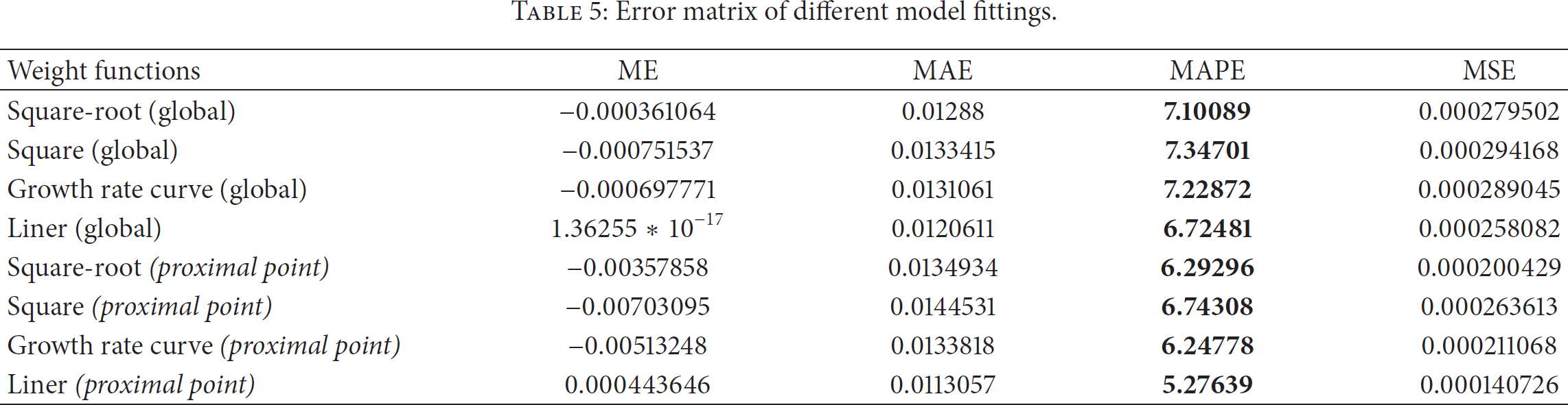
The forecast results of four different weighting functions can meet the basic requirements of the accuracy error of 10%. At the same time, we can know that the linear weight function has good fitting and forecasting effect on the experimental data. The linear weighting function is the optimal weight function for this forecast according to the statistics in Table 5.

6. Conclusion

This paper uses the change-point detection algorithm to divide travel time series into several patterns and set up forecasting model through ARIMA for different patterns based on massive data collected by the loop detectors on the roads. Different from traditional forecasting methods, it is easier to get the more optimized forecasting result than to obtain it by using the global search because the different intervals in same pattern have similar statistical characteristics of the mean and variance. In the process of dividing the travel time series, the calculation of algorithm is complicated and the derivation of control parameters is only obtained by experiments, which still needs research in the future.

Footnotes

Conflict of Interests

The authors declare no conflict of interests.

Authors' Contribution

Guangyu Zhu designed the forecasting model of travel time based on the change-point detection algorithm and wrote the paper; Li Wang designed the preprocessing algorithm and performed the data preprocess and revised the paper. Peng Zhang and Kang Song analyzed the data.

Acknowledgments

This work is supported by the National Science Foundation of China (nos. 61572069 and 61503022), the Fundamental Research Funds for the Central Universities (no. 2014JBM211), the Open Project Program of Key Laboratory of System Control and Information Processing, Ministry of Education, Shanghai Jiaotong University (no. Scip201507), Beijing Municipality Key Laboratory of Urban Traffic Operation Simulation and Decision Support, Beijing Transportation Research Center, the project of the Department of Traffic and Transportation of Hebei Province (no. A0201-150505), and The National Key Technology Support Program (no. 2014BAG01B02).

References

Z.-P.

Liu

Y.-C.

Liu

F.-Q.

An improved adaptive exponential smoothing model for short-term travel time forecasting of urban arterial street

Acta Automatica Sinica 2008 34 11 1404 1409

10.3724/sp.j.1004.2008.01404

2-s2.0-57249106547

Hollander

Liu

Estimation of the distribution of travel times by repeated simulation

Transportation Research Part C: Emerging Technologies 2008 16 2 212 231

10.1016/j.trc.2007.07.005

2-s2.0-38849085706

Jiang

G.-Y.

Technologies and Application of the Identification of Road Traffic Condition

Beijing, China

Communications Press

2004 (Chinese)

Gramaglia

Bernardos

C. J.

Calderon

Virtual induction loops based on cooperative vehicular communications

Sensors 2013 13 2 1467 1476

10.3390/s130201467

2-s2.0-84875181325

Zhang

Rice

J. A.

Short-term travel time prediction

Transportation Research Part C 2003 11 3-4 187 210

10.1016/s0968-090x(03)00026-3

2-s2.0-0042664086

Mori

Mendiburu

Álvarez

Lozano

J. A.

A review of travel time estimation and forecasting for Advanced Traveller Information Systems

Transportmetrica A: Transport Science 2015 11 2 119 157

10.1080/23249935.2014.932469

2-s2.0-84921438905

Vlahogianni

E. I.

Karlaftis

M. G.

Golias

J. C.

Short-term traffic forecasting: where we are and where we're going

Transportation Research Part C: Emerging Technologies 2014 43 part 1 3 19

10.1016/j.trc.2014.01.005

2-s2.0-84902550333

Shao

Zhang

A study of route travel time forecast method based on real data of urban expressway network

China Civil Engineering Journal 2003 36 1 16 20

Chilukuri

B. R.

Laval

J. A.

Guin

Microsimulation-based framework for freeway travel time forecasting

Transportation Research Record 2014 2470 34 45

10.3141/2470-04

10.

Yao

Zhang

A new algorithm of short—term travel time prediction for urban expressway

Journal of Wuhan University of Technology (Transportation Science & Engineering) 2013 6 1133 1137

11.

Zhao

Wang

Liu

Prediction of expressway travel time based on adaptive interpolation kalman filtering

Journal of South China University of Technology 2014 2 109 115

12.

Gui

Trip travel time forecasting based on selective forgetting extreme learning machine

Mathematical Problems in Engineering 2014 2014 7

829256

10.1155/2014/829256

13.

Jou

Y.-J.

Wen

Y.-H.

Lee

T.-T.

Cho

H.-J.

Missing data treatment on travel time estimation for ATIS

Proceedings of the IEEE International Conference on Systems, Man and Cybernetics (SMC ′03)

October 2003

Washington, DC, USA

IEEE

102 107

10.1109/ICSMC.2003.1243799

14.

Wang

A new method of real-time information collection in intelligent transportation system

Systems Engineering 2005 23 2 86 89

15.

Cai

Duan

Bourgeois

A. G.

Delay efficient opportunistic routing in asynchronous multi-channel cognitive radio networks

Journal of Combinatorial Optimization 2015 29 4 815 835

10.1007/s10878-013-9623-y

MR3327409

ZBL1321.90032

2-s2.0-84877631500

16.

VanLint

J. W. C.

Zijpp

N. J.

An improved travel time estimation algorithm using dual-loop detectors

Proceedings of the Annual Meeting of the Transportation Research Board

2003

Washington, DC, USA

17.

Cai

Goebel

Lin

Size-constrained tree partitioning: approximating the multicast k-tree routing problem

Theoretical Computer Science 2011 412 3 240 245

10.1016/j.tcs.2009.05.031

MR2789646

2-s2.0-78650610629

18.

Zhu

Yan

A kind of demand-forecasting model based on analysis of demand booming and principle of naive forecasting

Systems Engineering: Theory & Practice 2004 24 5 22 33

A Kind of Urban Road Travel Time Forecasting Model with Loop Detectors

Abstract

1. Introduction

2. Identification and Correction of the Loop Detector's Data

Algorithm 1.

3. Calculation of Travel Time Based on the Data from Loop Detector

Algorithm 2.

4. Forecast Model for Short-Term Travel Time Based on ARIMA

4.1. Change-Point Searching

Algorithm 3.

4.2. ARIMA Forecasting Model

5. Application Example

5.1. Preprocessing of the Massive Data from Loop Detectors

5.2. Calculation of Travel Time Parameters

5.3. Pattern Partition of Travel Time Series Based on Change-Point Analysis

5.4. Travel Time Forecasting Based on ARIMA Model

6. Conclusion

Footnotes

Conflict of Interests

Authors' Contribution

Acknowledgments

References