An Efficient Large-Scale Sensor Deployment Using a Parallel Genetic Algorithm Based on CUDA

Abstract

We have employed evolutionary computation to solve the optimization problem of sensor deployment in battlefield environments. A genetic algorithm has the advantage of delivering results of a higher quality than simple computational algorithms, but it has the drawback of requiring too much computing time. This study aimed not only to shorten the computing time to as close to real-time as possible by using the Compute Unified Device Architecture (CUDA) but also to maintain a solution quality that is as good as or better than the case when the proposed algorithm is not used. In the proposed genetic algorithm, parallelization was applied to speed up the fitness evaluation requiring heavy computation time. The proposed CUDA-based design approach for complex and various sensor deployments is validated by means of simulation. We parallelized two parts in Monte Carlo simulation for the fitness evaluation: moving lots of tested vehicles and calculating the probability of detection (POD) for each vehicle. The experiment was divided into CPU and GPU experiments depending on arithmetic unit types. In the GPU experiment, the results showed similar levels for the detection probability by GPU and CPU, and the computing time decreased by approximately 55-56 times.

1. Introduction

For several decades, a number of studies have been conducted on wireless sensor networks (WSNs), which have now become an essential component in the Internet of Things (IoT) in recent years [1]. WSNs consist of a large number of miniaturized low power sensors. Data is collected through these sensors wirelessly and stored in sinks, which then transfer the collected data to other networks.

Currently, WSNs are used in many areas such as real-time monitoring and automation in industrial fields, traffic surveillance and control, continuous health care, military target tracking, and environmental monitoring. Unlike commonly used wired and wireless networks, WSNs have many limitations to consider, such as battery life, computation capability, and communications. WSNs are very much application oriented; therefore, they require a customizable design according to application environments, and they require cross-layer optimization in the communication protocol stack. For this reason, WSNs require a wide range of research in multiple fields, including MAC, data routing, and transport protocols. WSN deployment is also considered one of the major WSN design factors and it has a significant effect on the performance measurement index, such as connectivity between sensors, efficient network coverage, and the network life cycle. Therefore, WSN deployment requires considerable research. In recent years, several well-organized survey studies on issues relating to WSN deployment have been published [1, 2]. In general, WSN is deployed in planned and random deployment methods. In random deployment, sensors are thrown into the region of interest (RoI) randomly, which could be in a disaster area or in war zones using airplanes. On the other hand, in the case of planned deployment, the location where sensors are deployed is determined beforehand to aim for maximum coverage, minimum power consumption, and strengthening of network connectivity. This deployment method is mainly used in border surveillance, facility intrusion detection, or procedural health care. It is also used in inaccessible ROIs into which sensors can be moved for deployment. In reality, various design objects, such as heterogeneous sensors and a large number of sensor deployments, characterize issues regarding planned deployment, which is an NP-hard problem [3]. Thus, it shows a tendency of rapidly increasing computing time to determine optimal solutions, depending on the size of the problem. To reduce the computing time, we applied parallelization techniques using GPU. There are four approaches for the planned deployment of WSNs: computational geometry, artificial potential field, genetic algorithm (GA), and particle swarm optimization. We have chosen the GA as our approach, which is a popular heuristic method.

There are several fundamental design factors in WSNs, such as the sensing model, sensor mobility, and network coverage and connectivity. Sensing models are divided into binary and probabilistic sensing models. In a binary sensing model [4, 5], a sensor has a simple fixed sensing radius and the object is detected if an object is present in the sensing radius; otherwise, it is not detected. In the probabilistic sensing model [6], various factors, such as noise and barriers, capable of affecting the accuracy of the sensor reading are taken into consideration. Depending on sensor mobility, WSNs are divided into static and mobile WSNs. A mobile WSN consists of sensors that have sensing, processing, communication, and mobile capabilities. A mobile WSN offers the advantage of redeployment and the ability to control sensor deployment after the initial random deployment and reconfiguration to restore networks that were disconnected because of energy depletion and environmental changes. However, a static WSN is assumed for this study. The WSN coverage can be classified into three methods: area coverage, point coverage, and barrier coverage [6, 7]. We have used the barrier coverage method [8], which deals with the general detection of all movement crossing over sensor barriers.

Korea presents special circumstances, because the country is divided into South and North. More than 70% of the terrain in Korea is mountainous, and guerrilla-like battles would be crucial to determine the fate of war. Mountainous terrain is characterized by the fact that it is extremely difficult to detect enemies with the naked eye at night and particularly it is almost impossible to precisely detect the size of enemies in a large area. To solve this problem, a variety of existing sensor deployment techniques can be applied, but it is still a highly complex problem to deploy sensors efficiently and rapidly while taking topographical characteristics into consideration [9]. We studied sensor deployment to detect movements of enemy troops and to enable us to cope with the unique circumstances presented by the mountainous terrain in Korea. As a result, we proposed the paralleled sensor deployment optimization method using GPU to obtain near real-time results by applying evolutionary computation.

The contributions of this paper include the following: (i) based on real environments, we used two types of sensors and three scenarios with different terrains and varied the number of sensors from 15 to 200 for comparison between CPU and GPU experiments; (ii) we not only shortened the computing time to as close to real-time as possible by using the CUDA but also maintained solution qualities that are as good as the results shown in the CPU test; (iii) we took an elaborated parallelized approach based on CUDA for complex and various sensor deployments.

The remainder of this paper is organized as follows: Section 2 explains CUDA and generational GA. Section 3 introduces related work for our subject handled in this paper. In Section 4, we present the problem definition and in Section 5 we explain the proposed parallel GA. Section 6 describes the environments of our experiment and Section 7 analyzes the results. The paper ends with conclusions in Section 8.

2. Preliminaries

2.1. CUDA (Compute Unified Device Architecture)

In November 2006, NVIDIA introduced CUDA [11], a general purpose parallel computing platform and programming model that leverages the parallel compute engine in NVIDIA GPUs to solve many complex computational problems in a more efficient way than on a CPU. CUDA comes with a software environment that allows developers to use C as a high-level programming language. Other languages, application programming interfaces, or directives-based approaches are supported, such as FORTRAN, DirectCompute, and OpenACC.

The advent of multicore CPUs and many-core GPUs means that mainstream processor chips are now parallel systems. Furthermore, their parallelism continues to scale with Moore's law. The challenge is to develop application software that transparently scales its parallelism to leverage the increasing number of processor cores, much as 3D graphics applications transparently scale their parallelism to many-core GPUs with widely varying numbers of cores. The CUDA parallel programming model is designed to overcome this challenge while maintaining a low learning curve for programmers familiar with standard programming languages such as C. At its core are three key abstractions—a hierarchy of thread groups, shared memories, and barrier synchronization—that are simply exposed to the programmer as a minimal set of language extensions.

These abstractions provide fine-grained data parallelism and thread parallelism, nested within coarse-grained data parallelism and task parallelism. They guide the programmer to partition the problem into coarse subproblems that can be solved independently in parallel by blocks of threads, and each subproblem into finer pieces that can be solved cooperatively in parallel by all threads within the block. This decomposition preserves language expressivity by allowing threads to cooperate when solving each subproblem and at the same time enables automatic scalability. Indeed, each block of threads can be scheduled on any of the available multiprocessors within a GPU, in any order, concurrently or sequentially, such that a compiled CUDA program can be executed on any number of multiprocessors, and only the runtime system needs to know the physical multiprocessor count.

This scalable programming model allows the GPU architecture to span a wide market range by simply scaling the number of multiprocessors and memory partitions: from the high-performance enthusiast GeForce GPUs and professional Quadro and Tesla computing products to a variety of inexpensive, mainstream GeForce GPUs.

2.2. Genetic Algorithm

Algorithm 1 shows the pseudocode of a typical GA [12]. In this algorithm, if we define that n is the number of solutions in the population, we randomly create n new solutions. The evolution starts from the population of completely random individuals and the fitness of the whole population is determined. Each generation consists of several operations such as selection, crossover, mutation, and replacement. All individuals in the current population are replaced with new individuals to form a new population. Finally, this generational process is repeated until a termination condition has been reached. In a typical GA, the whole number of individuals in a population and the number of reproduced individuals are fixed at n and k, respectively. The percentage of individuals who will be copied to the new generation is defined as the ratio of the number of new individuals to the size of the parent population, $k/n$ , which we termed the “generation gap.”

Algorithm 1:Pseudocode of a typical genetic algorithm.

Create an initial population of size n;

repeat  {

 for   $i=1$   to  k  {

  choose ${\mathrm{p}\mathrm{a}\mathrm{r}\mathrm{e}\mathrm{n}\mathrm{t}}_1$ and ${\mathrm{p}\mathrm{a}\mathrm{r}\mathrm{e}\mathrm{n}\mathrm{t}}_2$ from the population;

   ${\mathrm{o}\mathrm{f}\mathrm{f}\mathrm{s}\mathrm{p}\mathrm{r}\mathrm{i}\mathrm{n}\mathrm{g}}_i$  = crossover ( ${\mathrm{p}\mathrm{a}\mathrm{r}\mathrm{e}\mathrm{n}\mathrm{t}}_1$ , ${\mathrm{p}\mathrm{a}\mathrm{r}\mathrm{e}\mathrm{n}\mathrm{t}}_2$ );

   ${\mathrm{o}\mathrm{f}\mathrm{f}\mathrm{s}\mathrm{p}\mathrm{r}\mathrm{i}\mathrm{n}\mathrm{g}}_i$  = mutation ( ${\mathrm{o}\mathrm{f}\mathrm{f}\mathrm{s}\mathrm{p}\mathrm{r}\mathrm{i}\mathrm{n}\mathrm{g}}_i$ );

 }

 replace (population, [ ${\mathrm{o}\mathrm{f}\mathrm{f}\mathrm{s}\mathrm{p}\mathrm{r}\mathrm{i}\mathrm{n}\mathrm{g}}_1,{\mathrm{o}\mathrm{f}\mathrm{f}\mathrm{s}\mathrm{p}\mathrm{r}\mathrm{i}\mathrm{n}\mathrm{g}}_2,\dots ,{\mathrm{o}\mathrm{f}\mathrm{f}\mathrm{s}\mathrm{p}\mathrm{r}\mathrm{i}\mathrm{n}\mathrm{g}}_k$ ]);

}  until (stopping condition);

return the best solution;

In this study, we use a generational GA of which generation gap is 1. Figure 1 shows the process of our GA of which each part is briefly described in Table 1.

Table 1

GA used in the experiment.

GA parameters	Descriptions
Encoding	A vector of integer pairs (2D coordinates).
Population initialization	Creation of m random solutions.
Selection	Once $2^t$ solutions are selected randomly from the solution group, the best quality solution is chosen ( $t=3$ ).
Crossover	Creating an offspring by the genetic recombination of two parents. Each integer pair (a grid point) is randomly copied from the first or the second parent.
Mutation	Changing each gene of the offspring at the rate of 5 percent. Each integer pair (a grid point) in the offspring is randomly selected, and each integer value of the pair is added or subtracted by a small amount.
Replacement	If the solution quality of an offspring is better than that of the worst individual in the population, we replace it with the worst one.

Figure 1

Flow chart of the proposed generational GA.

3. Related Work

We have studied sensor deployment using a GA from a number of studies on WSNs. Table 2 compares studies that aimed to solve WSN deployment problems by using the GA.

Table 2

Comparison between genetic-based algorithms for WSN deployment.

Algorithm	Type of GA	Objective(s)	Type of sensors	Encoding	Sensing model
Yoon and Kim [13]	Normalized	(i) Maximize coverage	Heterogeneous	Integer	Deterministic
Kima et al. [14]	Generational	(i) Minimize travel time, find optimal location of sensors	Homogeneous	Binary	Probabilistic
Shi and Zhou [15]	Niche (real-coded)	(i) Maximize coverage	Homogeneous	Real-number	Deterministic
Unaldi et al. [16]	Generational, steady-state	(i) Maximize the quality of coverage of a WSN	Homogeneous	Integer	Probabilistic
Jourdan and de Weck [17]	Standard, multiobjective	(i) Maximize coverage (ii) Maximize lifetime	Homogeneous	Real-number	Deterministic
Jourdan and de Weck [18]	Standard, multiobjective	(i) Maximize coverage (ii) Maximize survivability (iii) Minimize number of sensors	Homogeneous	Real-number	Deterministic
Carter and Ragade [19]	Microbial	(i) Cover a set of target points (ii) Minimize number of sensors	Heterogeneous; (acoustic and image)	Binary	Deterministic
Carter and Ragade [20]	Microbial	(i) Cover a set of target points (ii) Minimize number of sensors	Homogeneous; (infrared)	Binary	Probabilistic
Deif and Gadallah [21]	Variable-length	(i) Cover a set of target points (ii) Maximize coverage (iii) Minimize cost	Heterogeneous; (nonisotropic)	Integer	Deterministic
Ta et al. [7]	Generational	(i) Minimize number of sensors	Homogeneous	Integer	Deterministic
Indhumathi and Venkatesan [22]	Generational	(i) Maximize coverage	Heterogeneous	Binary	Deterministic

A study by Yoon and Kim [13] proposed an efficient GA for the solution of the maximum coverage sensor deployment problem (MCSDP) with a maximum detection area. The authors created a novel normalization method, which was especially developed for the MCSDP with efficient evaluation functions and they proposed a novel sensor deployment methodology that was suited to the characteristics of the GA. They used a binary sensing model and diversified a sensing type and the radius of the detection range. In the MCSDP, the same solution was obtained from various types of representations, because the sizes of the genotype and phenotype spaces differed from each other, thereby causing degradation of execution performance, which was then alleviated by using the proposed normalization method. The evaluation functions derived results by combining the detection ranges of all sensors. In their experiment, in which the GA was used, the number of samples was set to 100,000. Further, once the final solution was obtained, the number of samples was set to 1 million to increase the accuracy of the result by recalculating it, thereby increasing its efficiency. Furthermore, as the generation of the GA evolved, the number of samples was increased gradually in the experiment, thereby reducing the computing time approximately by half, and achieving considerable performance improvement in terms of quality.

Kim et al. [14] studied methods for increasing the accuracy of time measurements for running vehicles on the highway. Previously, a travel time was estimated based on speed data measured via fixed sensors, but it was inaccurate, because it differed from the actual travel time. The authors took the characteristics of the highway (interchange connections, exits, and accidents) into consideration in the experiment as well as various setup options depending on the traffic volume, time of day, and incident duration. In the experiment, a microscopic traffic simulation model and GA were employed. The authors reduced the experimental time dramatically by omitting the simulation process, which was required every time when measuring fitness, instead of using an evaluation method of travel time via the speed data measured according to sensor positions produced from simulation results using the maximum number of sensors. The maximum number of sensors was 594 sensors and the gap between sensors was 76.2 m. The total distance in the experimental section was approximately 47.044 km. Binary encoding of 594 bits, which corresponded to the maximum number of sensors, was used. An activated sensor was indicated by bit 1, while an inactivated sensor was indicated by bit 0. In the experimental results, the error of travel time estimation was reduced to less than 10% and showed a better accuracy over 90% than existing measurement methods for most traffic situations. The best performance was revealed when using 60 sensors.

In a study by Shi and Zhou [15], a two-step strategy was used: the quality of the initial solution was increased up to a certain level using virtual force (VF) and then sensor deployment was optimized using a GA. They used 30 fixed sensors and 20 mobile sensors in a 100 × 100 area and 20 mobile sensors were used for optimal sensor deployment by means of VF and GA. The experiment was divided into VF, real-coded GA (RCGA), virtual force GA (VFGA), virtual force crossover GA (VFCGA), and virtual force mutation GA (VFMGA). The mean probability of detection (POD) of the experimental result showed the performance of VF, RCGA, VFGA, VFCGA, and VFMGA to be 83.79%, 96.53%, 97.53%, 95.83%, and 95.17%, respectively, indicating that VFGA performed the best.

Unaldi et al. [16] studied an optimal sensor deployment method in which a wavelet-transform- (WT-) based mutation operator was applied to a steady-state GA (S-GA) in three-dimensional (3D) terrain. Their proposed algorithm maximized the detection area by using a probabilistic sensing model and line of sight (LOS) algorithm proposed by Bresenham. The LOS algorithm can perform a relatively fast computation because it does not require interpolation computation in 3D environments. The sensing target area is divided into subregions depending on the number of sensors, and a subregion is composed of multiple pixels and a sensor is positioned at a specific pixel. The representation of each solution consists of a subregion and pixel numbers. When the specific detected pixel was within sensing range and there was a LOS between two pixels, then it was regarded as detected. This means that there was a height difference between a pixel located where a specific sensor was located and the detected pixel due to 3D terrain characteristics, and a virtual line was drawn between two pixels. If there was no pixel that went beyond that virtual line, it was regarded as detected. A single-point cross-operation was used, and a random mode and a WT-based attractiveness mode were compared for mutation operation. Furthermore, the WT-based mutation operation was divided into a method allowing a sensor to move only within a subregion and a method allowing a sensor to move between subregions, and the two methods were compared. The generational GA and S-GA were also compared. The S-GA experiment, in which the location of the sensor was set up to enable it to move between subregions and used a WT-based mutation operator, had the highest average POD of 76.3%.

Jourdan and de Weck [17] employed multiobjective GA (MOGA) to achieve the optimal deployment of n fixed sensors in a 2D plain. Their objectives were to maximize the coverage and lifetime of the WSNs. They used a binary sensing model and configured all sensors to have the same communication radius and sensing radius. Representation of solutions was expressed in a coordinate set of all sensors and each solution was ranked according to its area coverage and lifetime. Real-number encoding and random single-point crossover were used. In [18], Jourdan and de Weck applied the results of their study to three specific surveillance scenarios. The first scenario had three objectives: coverage maximization, minimization of deployed sensors, and maximization of distance between deployed sensor and hostile building under surveillance to ensure the maximum survival of networks. The objectives of the second and third scenarios were to minimize the number of deployed sensors while maximizing WSN coverage. The difference between the second and third scenarios was the different coverage type. The barrier coverage was maximized in the second scenario, while the area coverage was maximized in the third scenario. The experimental results showed samples of a pareto optimal set in nondominated deployments for each scenario, and the results offered guidance as to how trade-off information between competing objectives should be presented to a network designer. Their study had the advantage of being flexible enough to apply the result to design objectives of various sets, but their study had two drawbacks. First, it could derive incorrect results with a low accuracy due to the use of a binary sensing model. Second, it lacked practicality as their study assumed RoIs that only consisted of plains without obstacles.

Carter and Ragade [20] aimed to solve the problem by covering the target locations (target points) of a finite set by using predetermined sensors. They attempted to solve two deployment objectives (i.e., to minimize the number of deployed sensors and guarantee coverage of all target points) by using microbial GA [23]. They used two sensors: acoustic and image sensors. For acoustic sensors, a binary sensing model was applied, whereas the field-of-view metric [24] was applied for image sensors. Their study extended a previous study [19] by adding probabilistic coverage determination methods.

Feng et al. [25] studied the optimal placement of pyroelectric infrared (PIR) sensors in developing the infrared motion sensing system for human motion localization. They used a GA in optimizing both the deployment and the modulated field of view of the PIR sensors for improving the localization performance. The average and maximum localization errors were used to evaluate the localization performance. The numerical analysis was also presented to offer guidance on the searching spaces of the design parameters in implementing GA optimization.

Watfa and Commuri [26] studied the optimal 3-dimensional sensor deployment strategy. They rigorously analyzed the deployment problem in a 3D space in WSNs. They tried to solve the problem of determining the minimum number of sensor nodes that guarantee complete coverage. A regular hexagonal lattice arrangement was applied to solve the problem. In the present study, a real terrain was divided into a 2D grid and aimed to use optimal sensor deployment capable of maximizing the detection of moving vehicles. We took the topographical characteristics into consideration and acoustic and FLIR sensors were used. In the present study, a Monte Carlo simulation method was employed and a large performance improvement was achieved by using parallel processing with GPUs. The parts to which parallel processing was applied were POD computation in the fitness function and POD computation due to movement of the vehicle. We aimed to improve the practical applicability by reflecting the real topographical information and overcoming the disadvantage of a GA, namely, slow computing speed.

4. Problem Definition

4.1. Terrain and Obstacles

Real terrain of 5 km by 5 km was divided according to a 50 × 50 grid (Figure 2) and the size of each grid point was set to 100 m × 100 m. For a grid point in hilly terrain, the detection capacity of the sensor was reduced by a certain value [9, 10]. We used three different scenarios: one of them is plain and the other two are with hilly terrain. Figure 3 shows the terrain of Scenarios 1 and 2 and the yellow parts represent hilly terrain. A POD at each grid point was calculated after the sensors were deployed and PODs were calculated by using a setting that enabled a vehicle to be detected or not detected based on the PODs whenever a vehicle passed through each grid point. Figure 4 shows the approximate location of Figures 3(a) and 3(b) on a map of the Korean Peninsula.

Figure 2

Grid model of the battlefield for sensor deployment.

Figure 3

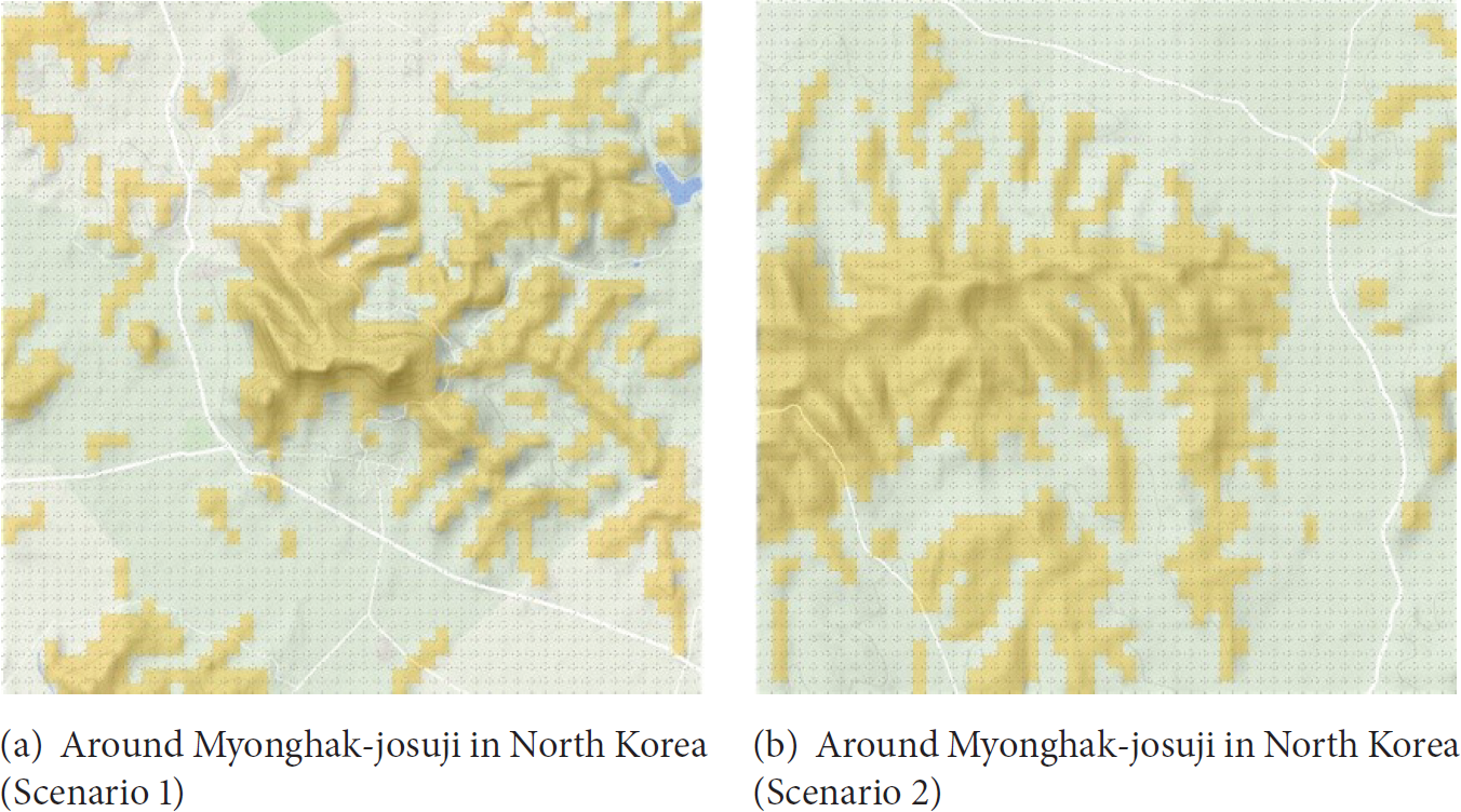
Map where hilly terrain information is applied.

Figure 4

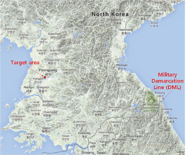
Location of DML and experimental target area on Korean Peninsula.

In Section 6.1, we give a detailed explanation of our modeling and simulator. In the modeling of Scenarios 1 and 2, we represented the grid model of Figure 2 as a two-dimensional integer array having 50 × 50 sizes. If a grid point is higher than 100 meters above the sea level, the element of the array has value 1 as hill, otherwise 0 as plain. We developed a sensor deployment simulator using C and CUDA-C languages on NVIDIA CUDA platform 7.0.

4.2. Type of Sensors and Detectable Range by Sensor

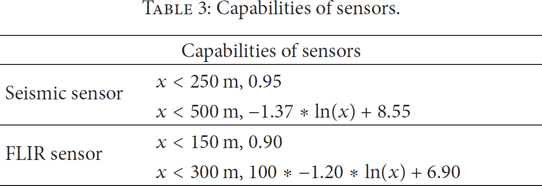
Seismic and FLIR sensors as shown in Table 3 were used for the experiment [10]. For seismic sensors, if the distance between the grid point and sensor was less than 250 m, a detectable range was set at 95%, if a distance was less than 500 m and larger than 250 m, a range was set at $(-1.37\times \ln \left(\mathrm{d}\mathrm{i}\mathrm{s}\mathrm{t}\mathrm{a}\mathrm{n}\mathrm{c}\mathrm{e}\right)+8.55)$ , and if the distance was more than 500 m, the range was set at 0%. For FLIR sensors, if the distance between the grid point and the sensor was less than 150 m, a detectable range was set at 90%, if the distance was less than 300 m and larger than 150 m, the range was set at $(-1.20\times \ln \left(\mathrm{d}\mathrm{i}\mathrm{s}\mathrm{t}\mathrm{a}\mathrm{n}\mathrm{c}\mathrm{e}\right)+6.90)$ , and if the distance was more than 300 m, the range was set at 0%.

Table 3

Capabilities of sensors.

Capabilities of sensors
Seismic sensor	$x<\mathrm{250}$  m, 0.95
	$x<\mathrm{500}$  m, $-\mathrm{1.37}\ast \ln (x)+\mathrm{8.55}$
FLIR sensor	$x<\mathrm{150}$  m, 0.90
	$x<\mathrm{300}$  m, $\mathrm{100}\ast -\mathrm{1.20}\ast \ln (x)+\mathit{6.90}$

4.3. POD Calculation at Each Grid Point

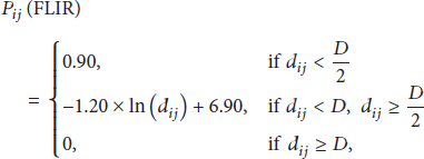
After a certain number of grid sensors were deployed, the distance between a single grid point and sensors is calculated. Equations (1) and (2) mean the probabilities that a single grid point could be detected by a seismic sensor and an FLIR sensor around the grid point, respectively. Each probability is accumulated for the process of (3), and this accumulated value is POD of the grid point. An example of POD calculation is shown in Section 5.1, in Algorithm 3 and Figure 5. Equation (3) represents the POD equation for a single grid point, where $p_j$ is the POD at each grid point, n is the number of deployed sensors, and k is a sequence number of the grid point (0–2499). In the case of $j\in \left\{\mathrm{1,2},\dots ,m\right\}$ , $p_j$ is the probability for detecting a target at grid point j and $d_{ij}$ is the distance between sensor i and grid point j. Constant D is 500 in the case of seismic sensors, and 300 in the case of FLIR sensors. In the POD computation, the condition of the hilly terrain was taken into consideration, applying the reduction rate of 65% when the grid point was on a hillside [9, 10]:

$$\begin{array}{cc}& P_{ij}\left(\mathrm{s}\mathrm{e}\mathrm{i}\mathrm{s}\mathrm{m}\mathrm{i}\mathrm{c}\right)=\left\{\begin{array}{cc}\mathrm{0.95},\hfill & \text{if\hspace{0.17em}\hspace{0.17em}}{d}_{ij}<\frac{D}{\mathrm{2}}\hfill \\ -\mathrm{1.37}\times \ln \left(d_{ij}\right)+\mathrm{8.55},\hfill & \text{if\hspace{0.17em}\hspace{0.17em}}{d}_{ij}<D,\hspace{0.17em}\hspace{0.17em}{d}_{ij}\ge \frac{D}{\mathrm{2}}\hfill \\ \mathrm{0},\hfill & \text{if\hspace{0.17em}\hspace{0.17em}}{d}_{ij}\ge D,\hfill \end{array}\right.\end{array}$$

(1)

$$\begin{array}{cc}& P_{ij}\left(\mathrm{F}\mathrm{L}\mathrm{I}\mathrm{R}\right)=\left\{\begin{array}{cc}\mathrm{0.90},\hfill & \text{if\hspace{0.17em}\hspace{0.17em}}{d}_{ij}<\frac{D}{\mathrm{2}}\hfill \\ -\mathrm{1.20}\times \ln \left(d_{ij}\right)+\mathrm{6.90},\hfill & \text{if\hspace{0.17em}\hspace{0.17em}}{d}_{ij}<D,\hspace{0.17em}\hspace{0.17em}{d}_{ij}\ge \frac{D}{\mathrm{2}}\hfill \\ \mathrm{0},\hfill & \mathrm{i}\mathrm{f}\hspace{0.17em}\hspace{0.17em}{d}_{ij}\ge D,\hfill \end{array}\right.\end{array}$$

(2)

$$\begin{array}{cc}& P\left(p_j\right)=P_{\mathrm{1}j}+{\displaystyle \sum }_{i=\mathrm{2}}^n\hspace{0.17em}{\displaystyle \prod }_{k=\mathrm{1}}^{i-\mathrm{2}}\left(\mathrm{1}-P_{ij}\right).\end{array}$$

(3)

Figure 5

Method for parallelizing POD calculation of each cell in the GPU.

4.4. POD Calculation

For each moving vehicle x position was selected randomly from 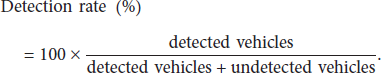$x=\left\{\mathrm{0,1},\dots ,49\right\}$ and it was moved in an increasing direction of y, as shown in Figure 6. Whenever a vehicle passed through each grid point, the POD at each grid point was compared with the random value and if the POD was larger, then it was regarded as detected. The detected vehicles value was increased when it was detected while y was within a range of 0–47; otherwise, the undetected vehicles value was increased when it was not detected, calculating the POD (fitness) of each solution as indicated in

$$\begin{array}{cc}& \text{Detection\hspace{0.17em}\hspace{0.17em}rate\hspace{0.17em}\hspace{0.17em}}\left(\%\right)=\mathrm{100}\times \frac{\text{detected\hspace{0.17em}\hspace{0.17em}vehicles}}{\text{detected\hspace{0.17em}\hspace{0.17em}vehicles}+\text{undetected\hspace{0.17em}\hspace{0.17em}vehicles}}.\end{array}$$

(4)

Figure 6

Probability of possible moving direction of vehicles and of moving direction [9, 10].

5. CUDA-GA Design

5.1. Parallel POD Calculation

In the CPU experiments, the process requiring the longest computation time was the fitness evaluation which consisted of two parts: POD calculation of each grid point and calculation of detection rate according to vehicle movement. Table 4 and Figure 5(b) show the structure of grid and block. A grid has 50 × 100 × 1 blocks and each block has 50 × 1 × 1 threads. A thread was in charge of a POD calculation.

Table 4

Grid and block dimensions of POD calculation.

	Dimensions
Blocks per grid	$$\left(x,y,z\right)=\left(\mathrm{50,100,1}\right)$$
Threads per block	$$\left(x,y,z\right)=\left(\mathrm{50,1},\mathrm{1}\right)$$

Algorithm 2 shows the pseudocode of POD kernel function on NVIDIA CUDA platform. It concurrently calculates every POD per generation. The return values of the kernel function are 250,000 PODs per generation. Coordinates $(x,y)$ of all sensors are stored in two one-dimensional arrays, respectively. sensors_x is the pointer of x-coordinate array and sensors_y is that of y-coordinate array. In the kernel function, the arrays are copied to shared memory which is shared by all threads in a block. The shared memory is very fast and reduces memory latency. $(c,r)$ is a coordinate of a grid point which has a POD. From the grid point $(c,r)$ , the distance with all sensors was calculated and sorted by ascending order. A POD is calculated by accumulating the probability calculated by (1) or (2) according to the order of sensors. It takes $O(n)$ time to copy system memory into GPU shared memory. The process of POD calculation at each grid point also takes $O(n)$ time. The total time complexity becomes a linear time with respect to the number of sensors.

Algorithm 2:Pseudocode of POD calculation.

// n: # of sensors;

// $x[1,\dots ,n]$ ,   $y[1,\dots ,n]$ : coordinates of sensors in system memory;

// $sx[1,\dots ,n]$ , $sy[1,\dots ,n]$ : coordinates of sensors in GPU shared memory;

//   ${gt}_{\mathrm{i}\mathrm{d}}$ : unique index of each thread in GPU;

// c: column number of a current grid point; r: row number of a current grid point

if threadIdx.x is zero then

  for  $i\leftarrow 0$  to  $n-1$  do

   $sx[i]\leftarrow x[i]$ ; $sy[i]\leftarrow y[i]$ ;

  end for

end if

_⁢_syncthreads(); // wait all threads in this block;

// sorting sensors in ascending distance order around the grid point ( $c,r$ );

POD ← 0.0; // POD: probability of detection at the grid point ( $c,r$ );

for  $i\leftarrow 0$  to  $n-1$  do

 d ← distance between the grid point ( $c,r$ ) and sensors [i];

 st ← kind of sensors [i]; // SEISMIC or FLIR

  if st is SEISMIC then

   if   $d\le \mathrm{250}$   then  $\mathrm{P}\mathrm{O}\mathrm{D}$   +=  $(1-\mathrm{P}\mathrm{O}\mathrm{D})\ast \mathit{0.95}$ ;

   else if   $d<\mathrm{500}$   then  $\mathrm{P}\mathrm{O}\mathrm{D}$   +=  $(1-\mathrm{P}\mathrm{O}\mathrm{D})\ast (-\mathit{1.3738}\ast \ln (d)+\mathit{8.5464})$ ;

   end if

  else if st is FLIR then

   if  $d\le \mathrm{150}$    then    $\mathrm{P}\mathrm{O}\mathrm{D}$   +=  $(1-\mathrm{P}\mathrm{O}\mathrm{D})\ast \mathit{0.90}$ ;

   else if  $d<\mathrm{300}$    then    $\mathrm{P}\mathrm{O}\mathrm{D}$   +=  $(1-\mathrm{P}\mathrm{O}\mathrm{D})\ast (-\mathit{1.2}\ast \ln (d)+\mathit{6.9})$ ;

   end if

  end if

end for

Algorithm 3:Example of POD calculation of a grid point.

(a) Probability of cell (4, 2) being detected by sensor (5, 1), which is located at the closest distance.

(b) Probability of not being detected at (a) × Probability of cell (4, 2) being detected by sensor (2, 2)

  which is the next closest distance.

(c) Probability of not being detected at (b) × Probability of cell (4, 2) being detected by sensor (6, 4)

  which is the next closest distance.

(d) Probability of not being detected at (c) × Probability of cell (4, 2) being detected by sensor (4, 6)

  which is the next closest distance.

The CPU experiment used a method that sequentially calculated the POD per generation for each solution. The calculated POD value was input into each grid point, and when a vehicle passed through the grid point, the probability of being detected was calculated by comparing the POD at each grid point with the newly generated random value, to determine whether the vehicle was detected or not. Figure 5(a) shows an example in which the POD is calculated at grid point $(x,y)=(\mathrm{4,2})$ when two seismic sensors and two FLIR sensors were deployed. Algorithm 3 shows the procedure for calculating the POD when the grid point is $(\mathrm{4,2})$ . The POD is the sum of probability values from (a) to (d). Figure 5(b) shows the setup of blocks and threads used to calculate the PODs in parallel at all grid points within the solution group. It consists of 50 blocks, each of which contains 50 threads, thereby enabling 2,500 PODs to be calculated simultaneously.

5.2. Calculation of Vehicle Movement in Parallel

Each vehicle was moved according to the moving direction probability in Figure 7, as shown in Figure 6. Each vehicle sequentially passes through the region of interest and vehicles have no interference with each other. In the GPU experiment, vehicles of all solutions (100 solutions × 30 vehicles) were moved in parallel to calculate the POD of each solution. Whenever a vehicle moves into other grid points, y-coordinate is changed. In the case that y-coordinate is larger than or equal to 47, the vehicle is regarded to have arrived at the destination as in [10].

Figure 7

Example of vehicle movement path passing through target area.

In the fitness evaluation of a solution, each of thirty vehicles independently passes through the region of interest in its own workspace, in parallel. Table 5 and Figure 8 show the structure of a grid and blocks of vehicle movements.

Table 5

Grid and block dimensions of vehicle movement.

	Dimensions
Blocks per grid	$$\left(x,y,z\right)=\left(\mathrm{100,1},\mathrm{1}\right)$$
Threads per block	$$\left(x,y,z\right)=\left(\mathrm{30,1},\mathrm{1}\right)$$

Figure 8

Vehicle movements for each thread in the GPU.

Algorithm 4 gives the pseudocode of calculating detection ratio according to the vehicle movements. $\mathrm{P}\mathrm{O}{\mathrm{D}}_{\mathrm{g}\mathrm{r}\mathrm{i}\mathrm{d}}$ is a variable of having 250,000 PODs in all solutions and it is given as a parameter. Whenever a vehicle moves into other grid points, we check whether or not the vehicle is detected. In the case that the vehicle is detected, the value of detected variable increases by 1, otherwise that of undetected variable increases by 1. Time complexity of Algorithm 4 is $O(r)$ , where r is the number of rows in given grid model.

Algorithm 4:Pseudocode of vehicle movements.

// detected: detected count, undetected: undetected count;

// x: column number of a current grid point;

// y: row number of a current grid point;

// $r\leftarrow$  random value $[0,\dots ,\mathrm{100}]$ ; $rf$  ← float random value [ $\mathit{0.0},\dots ,\mathit{1.0}$ ];

// ${\mathrm{P}\mathrm{O}\mathrm{D}}_{\text{grid}}$ : PODs of a grid;

//   $t_{\mathrm{i}\mathrm{d}}$ : unique id of each thread in a block;

repeat

  if $r\le 2$    then   y−−; // moving to back;

  else if    $r\le 7$    then ; // hold current position;

  else if    $r\le \mathrm{14}$    then   x−−; // moving to right;

  else if    $r\le \mathrm{21}$    then   x++; // moving to left;

  else if    $r\le \mathrm{43}$    then   x−−, $y++$ ; // moving to right and forward;

  else if    $r\le \mathrm{65}$    then   x++, $y++$ ; // moving to left and forward;

  else if    $r\le \mathrm{100}$    then   y++; // moving to forward;

  end if

  if    $\mathrm{P}\mathrm{O}{\mathrm{D}}_{\mathrm{g}\mathrm{r}\mathrm{i}\mathrm{d}}[t_{\mathrm{i}\mathrm{d}}]$ > rf   then detected++;

  else   undetected++;

  end if

until   ( $y<\mathrm{47}$ );

6. Experimental Setup

The performance was compared and evaluated by using a CPU and GTX970 GPU. If the number of degrees of freedom in the t distribution was 30 or larger, the approximation can be statistically meaningful in our experiments [27]. We performed 30 independent tests for this reason. All types of experiments were repeated 30 times and the mean and standard deviation of the optimal solution for each experiment were calculated to compare the quality of the solution. The time required to complete the experiments was measured by dividing the performance time into the GA execution time, evaluation function execution time, POD calculation time, and vehicle movement and POD calculation time, and the average of each execution time was calculated for the experimental results. For each solution, 30 vehicles were run to calculate the POD. The type of experiment was set as follows: First, it was divided into CPU and GPU experiments. Second it was divided into seismic and FLIR sensors, in which a different sensing range was specified for each sensor. Third, the number of deployed sensors was diversified by using 15, 25, 50, 100, 150, and 200 sensors. Finally, three topographical scenarios were used.

We used a general desktop computer to optimize sensor deployment on specific area of 5 km by 5 km. The price of the computer was around $500. We could improve computing speed using CUDA after an NVIDIA GeForce GTX 970 and a 500 W power supply unit were installed. The graphic card and the power supply unit cost about $700.

6.1. Test Environments

We developed a sensor deployment simulator using C and CUDA-C languages on NVIDIA CUDA platform 7.0. It has various setup options such as the types of arithmetic units, the number and types of sensors, and GA parameters. The simulator consists of three parts: one is a generational GA, another is the fitness function of CPU, and the third is that of GPU.

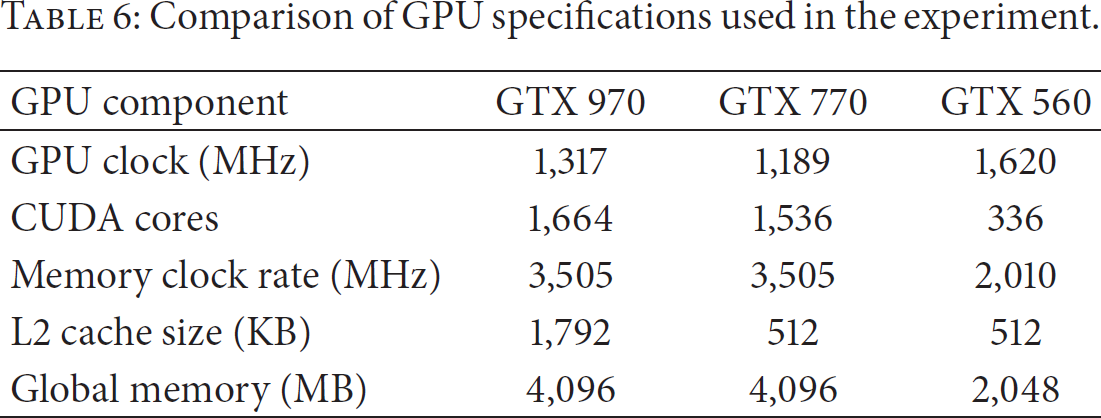
In the CPU experiment, a PC with Intel Core2 duo quad core 3.0 GHz processors and 4 GB memory was used. In the GPU experiment, NVIDIA GeForce GTX graphic cards were mounted in the same PC that was used in the CPU experiment. Table 6 shows the information for the three different GPUs used in our tests. The important factors are CUDA cores and L2 cache size. L2 cache is used in shared memory and registers. The L2 cache improves performance for the CUDA applications in the aspects of memory access patterns. NVIDIA GeForce GTX 970 has three times more L2 cache than the other two GPUs, and it can speed up in memory usage if we use L2 cache in an efficient way. CUDA cores are useful to process a lot of small tasks.

Table 6

Comparison of GPU specifications used in the experiment.

GPU component	GTX 970	GTX 770	GTX 560
GPU clock (MHz)	1,317	1,189	1,620
CUDA cores	1,664	1,536	336
Memory clock rate (MHz)	3,505	3,505	2,010
L2 cache size (KB)	1,792	512	512
Global memory (MB)	4,096	4,096	2,048

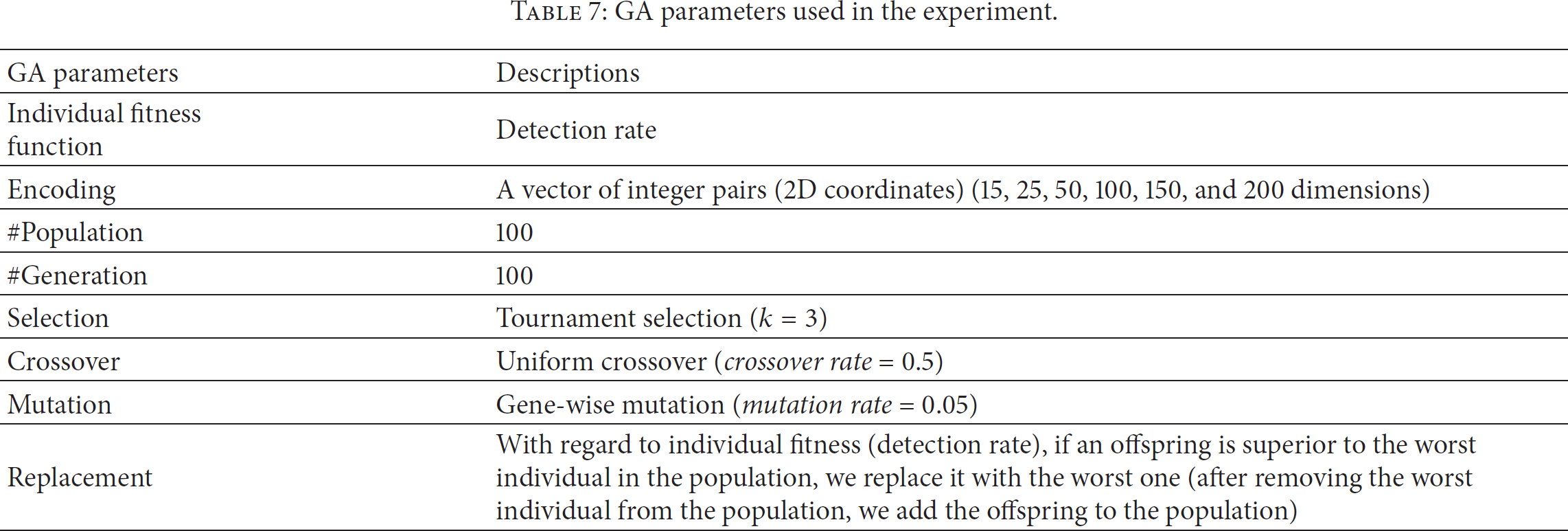
6.2. GA Parameters Configuration

Table 7 shows the configuration of the GA parameters for the experiment. The 2D grid was encoded by using a list of ( $x,y$ ) coordinates. The first part of the listed coordinates refers to seismic sensors, whereas the second part refers to the listed coordinate of the FLIR sensor.

Table 7

GA parameters used in the experiment.

GA parameters	Descriptions
Individual fitness function	Detection rate
Encoding	A vector of integer pairs (2D coordinates) (15, 25, 50, 100, 150, and 200 dimensions)
#Population	100
#Generation	100
Selection	Tournament selection ( $k=3$ )
Crossover	Uniform crossover (crossover rate= 0.5)
Mutation	Gene-wise mutation (mutation rate= 0.05)
Replacement	With regard to individual fitness (detection rate), if an offspring is superior to the worst individual in the population, we replace it with the worst one (after removing the worst individual from the population, we add the offspring to the population)

6.3. Maximum Coverage

The theoretically possible maximum coverage was calculated as follows. The POD was calculated for a single sensor, and the calculated PODs were summed, followed by division by the total number of grid points, 2,500. A single seismic sensor and a single FLIR sensor can cover 69 and 25 grid points maximally, respectively, as shown in Figure 9. The sum of the PODs at 69 grid points, each with a value larger than 0 based on a single seismic sensor, was 40.412 and it showed 1.616% of coverage. The sum of the PODs at 25 grid points, each with a value larger than 0 based on a single FLIR sensor, was 14.038 and it showed 0.561% of coverage. In (5), which calculates the maximum coverage, $C_{\mathrm{s}\mathrm{e}\mathrm{i}\mathrm{s}\mathrm{m}\mathrm{i}\mathrm{c}}$ was 1.616% and $C_{\mathrm{F}\mathrm{L}\mathrm{I}\mathrm{R}}$ was 0.561%. The parameter #cells represents the size of the grid, which was 2,500. #seismic was the number of seismic sensors and #FLIR was the number of FLIR sensors. Table 8 shows the theoretically possible maximum coverage calculated as per the number of sensors deployed using

$$\begin{array}{cc}& M=C_{\mathrm{s}\mathrm{e}\mathrm{i}\mathrm{s}\mathrm{m}\mathrm{i}\mathrm{c}}\times \frac{\#\mathrm{s}\mathrm{e}\mathrm{i}\mathrm{s}\mathrm{m}\mathrm{i}\mathrm{c}}{\#\mathrm{c}\mathrm{e}\mathrm{l}\mathrm{l}\mathrm{s}}+C_{\mathrm{F}\mathrm{L}\mathrm{I}\mathrm{R}}\times \frac{\#\mathrm{F}\mathrm{L}\mathrm{I}\mathrm{R}}{\#\mathrm{c}\mathrm{e}\mathrm{l}\mathrm{l}\mathrm{s}}.\end{array}$$

(5)

Table 8

Maximum coverage rate according to the number and type of sensors.

Instances	Seismic sensor	FLIR sensor	Coverage of seismic sensor (%)	Coverage of FLIR sensor (%)	Maximum coverage (%)
Instance 1	7	8	11.3	4.5	15.8
Instance 2	12	13	19.4	7.3	26.7
Instance 3	25	25	40.4	14.0	54.4
Instance 4	50	50	80.8	28.1	100
Instance 5	75	75	100	42.1	100
Instance 6	100	100	100	56.2	100

Figure 9

Coverage of a sensor.

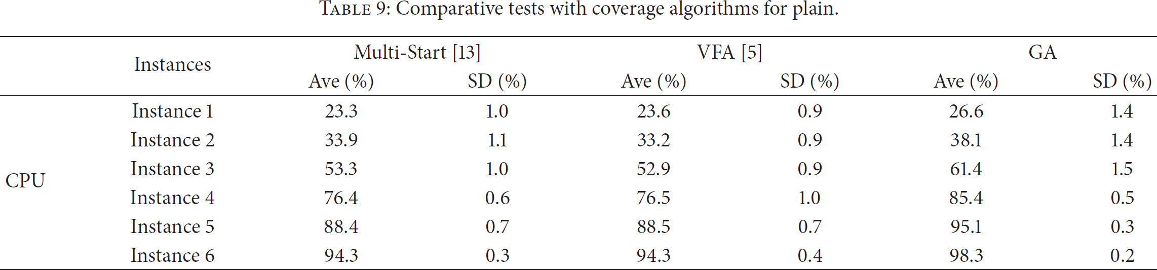
7. Experimental Results

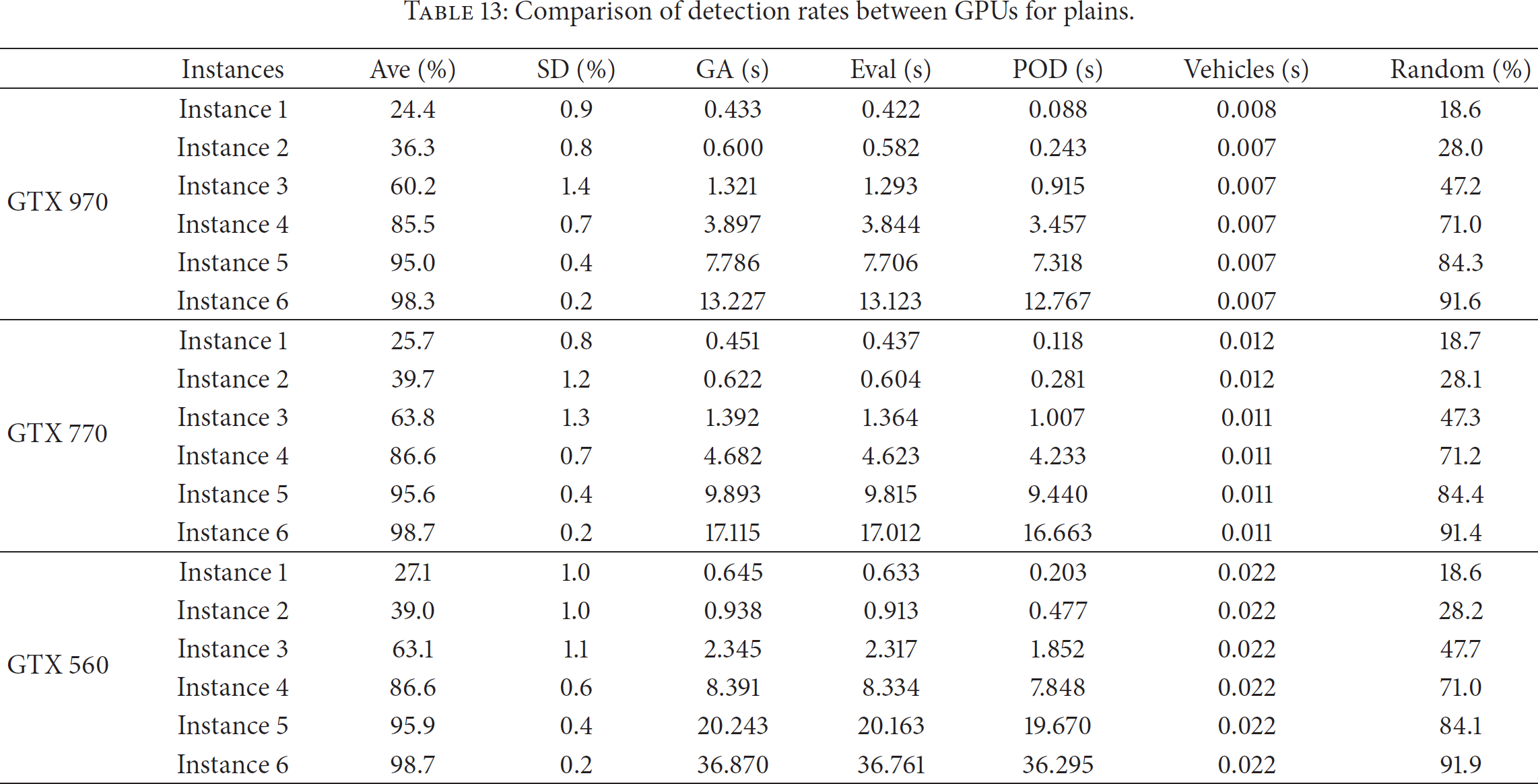
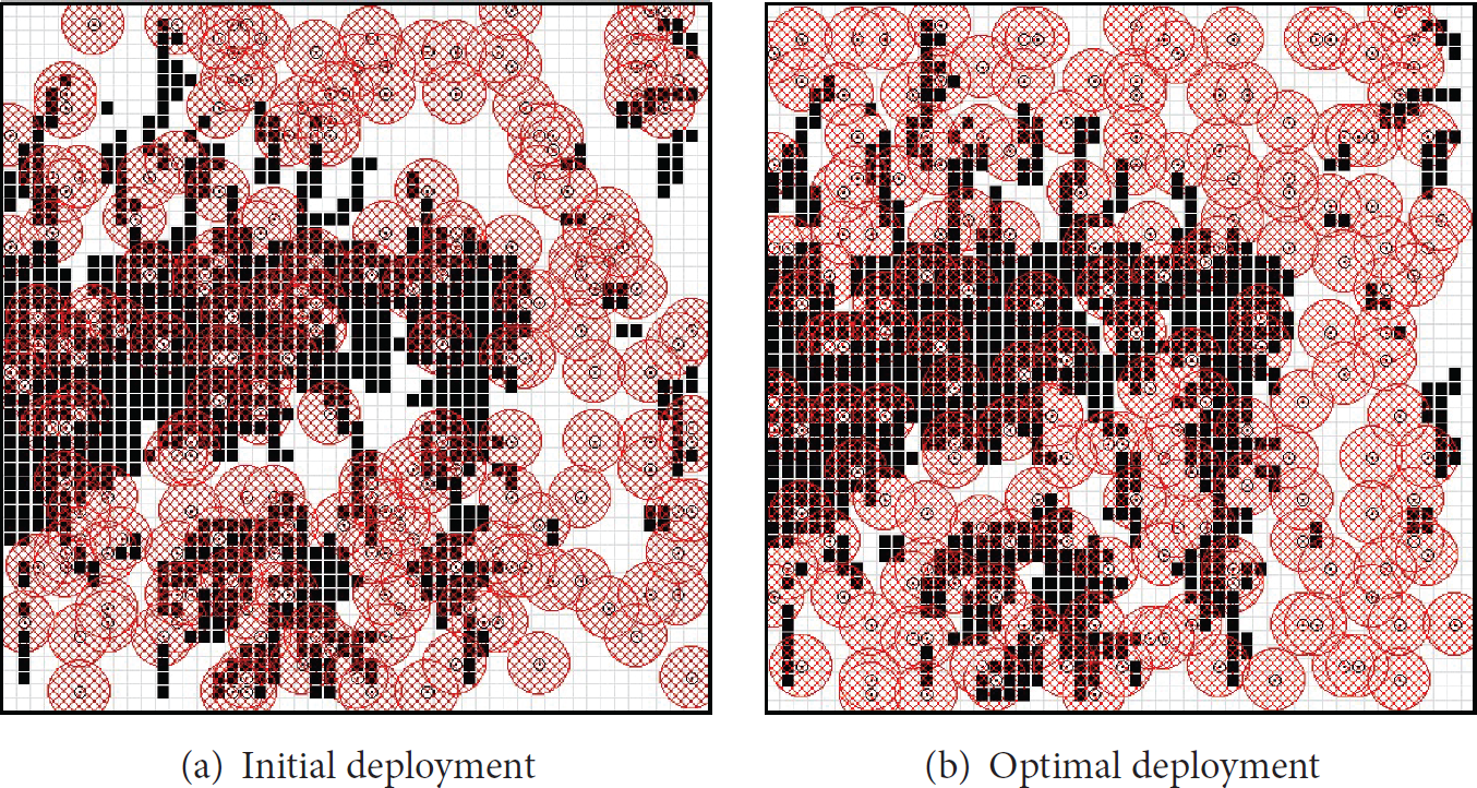
All values in Tables 9–13 are the average results of 30 experiments. Table 9 shows the results of comparative tests with coverage algorithms such as Multi-Start [13], VFA [5], and the proposed GA, which were obtained using the same computing time for fair comparison. The results of Multi-Start and VFA were superior to those of the initial random deployment, which are given in the last column of Table 10. Multi-Start showed better qualities than VFA when the number of sensors was 50 or under. However, in the case that the number of sensors was above 50, the qualities of VFA were better than or equal to those of Multi-Start. The proposed GA was the best among all tests. Tables 10–12 show experimental results according to the terrain type and the CPU and GPU results according to the number of deployed sensors. Tables 10–12 show that as the number of deployed sensors increased, the POD also increased constantly, while the standard deviation decreased gradually, indicating a conversion of the solution groups. Table 13 shows the comparative results of detection rates between GPUs for plains. Figure 16 shows computing time according to the number of vehicles in GPU tests. The computing time slightly increases even though the number of vehicles shows drastic change. The reason is that moving of vehicles is concurrently processed in CUDA. Figures 17–19 show the initial deployments and the optimal deployments, which were obtained by the proposed GA, of the tested scenarios. Initial deployment is a very important factor which influences the detection rates. We initially deployed sensors following a uniform distribution to make tests fair.

Table 9

Comparative tests with coverage algorithms for plain.

	Instances	Multi-Start [13]		VFA [5]		GA
		Ave (%)	SD (%)	Ave (%)	SD (%)	Ave (%)	SD (%)
CPU	Instance 1	23.3	1.0	23.6	0.9	26.6	1.4
	Instance 2	33.9	1.1	33.2	0.9	38.1	1.4
	Instance 3	53.3	1.0	52.9	0.9	61.4	1.5
	Instance 4	76.4	0.6	76.5	1.0	85.4	0.5
	Instance 5	88.4	0.7	88.5	0.7	95.1	0.3
	Instance 6	94.3	0.3	94.3	0.4	98.3	0.2

Table 10

Experimental results for plain.

	Instances	Ave (%)	SD (%)	GA (s)	Eval (s)	POD (s)	Vehicles (s)	Random (%)
GTX 970	Instance 1	24.4	0.9	0.433	0.422	0.088	0.008	18.6
	Instance 2	36.3	0.8	0.600	0.582	0.243	0.007	28.0
	Instance 3	60.2	1.4	1.321	1.293	0.915	0.007	47.2
	Instance 4	85.5	0.7	3.897	3.844	3.457	0.007	71.0
	Instance 5	95.0	0.4	7.786	7.706	7.318	0.007	84.3
	Instance 6	98.3	0.2	13.227	13.123	12.767	0.007	91.6
CPU	Instance 1	26.6	1.4	11.080	11.070	N/A	N/A	19.5
	Instance 2	38.1	1.4	25.950	25.936	N/A	N/A	29.1
	Instance 3	61.4	1.5	79.101	79.073	N/A	N/A	48.7
	Instance 4	85.4	0.5	237.074	237.022	N/A	N/A	72.7
	Instance 5	95.1	0.3	456.122	456.041	N/A	N/A	85.3
	Instance 6	98.3	0.2	743.208	743.108	N/A	N/A	92.7

∗Ave: average of detection rates, SD: standard deviation of detection rates, GA: computing time of genetic algorithm, Eval: fitness function computing time, POD: POD computing time, Vehicles: computing time according to vehicle movement, and Random: detection rates when random deployment is applied.

Table 11

Experimental results of Scenario 1.

	Instances	Ave (%)	SD (%)	GA (s)	Eval (s)	POD (s)	Vehicles (s)	Random (%)
GTX 970	Instance 1	22.3	0.8	0.433	0.423	0.089	0.008	16.8
	Instance 2	32.9	1.0	0.624	0.604	0.244	0.007	25.2
	Instance 3	53.7	1.0	1.349	1.316	0.915	0.007	42.2
	Instance 4	76.2	0.7	3.908	3.854	3.460	0.007	63.0
	Instance 5	84.7	0.4	7.793	7.716	7.320	0.007	74.9
	Instance 6	87.9	0.2	13.245	13.139	12.779	0.007	81.5
CPU	Instance 1	25.0	1.3	10.527	10.517	N/A	N/A	17.7
	Instance 2	35.5	1.3	25.360	25.345	N/A	N/A	26.2
	Instance 3	55.7	1.2	77.559	77.533	N/A	N/A	43.3
	Instance 4	77.8	1.0	232.520	232.469	N/A	N/A	64.7
	Instance 5	86.3	0.7	449.369	449.292	N/A	N/A	76.4
	Instance 6	89.9	0.3	728.997	728.892	N/A	N/A	82.9

Table 12

Experimental results of Scenario 2.

	Instances	Ave (%)	SD (%)	GA (s)	Eval (s)	POD (s)	Vehicles (s)	Random (%)
GTX 970	Instance 1	22.6	0.8	0.430	0.420	0.089	0.008	16.4
	Instance 2	33.3	1.0	0.595	0.578	0.243	0.007	24.7
	Instance 3	53.0	1.1	1.317	1.290	0.913	0.007	40.8
	Instance 4	74.6	0.7	3.903	3.851	3.459	0.007	62.0
	Instance 5	83.0	0.5	7.807	7.729	7.324	0.007	73.4
	Instance 6	86.3	0.4	13.246	13.139	12.780	0.007	80.2
CPU	Instance 1	25.1	1.3	10.482	10.472	N/A	N/A	17.3
	Instance 2	35.5	1.7	25.271	25.256	N/A	N/A	25.4
	Instance 3	54.7	1.1	77.486	77.460	N/A	N/A	42.6
	Instance 4	75.1	0.4	234.460	234.409	N/A	N/A	63.5
	Instance 5	84.0	0.2	449.728	449.652	N/A	N/A	75.1
	Instance 6	87.3	0.3	730.183	730.076	N/A	N/A	81.7

Table 13

Comparison of detection rates between GPUs for plains.

	Instances	Ave (%)	SD (%)	GA (s)	Eval (s)	POD (s)	Vehicles (s)	Random (%)
GTX 970	Instance 1	24.4	0.9	0.433	0.422	0.088	0.008	18.6
	Instance 2	36.3	0.8	0.600	0.582	0.243	0.007	28.0
	Instance 3	60.2	1.4	1.321	1.293	0.915	0.007	47.2
	Instance 4	85.5	0.7	3.897	3.844	3.457	0.007	71.0
	Instance 5	95.0	0.4	7.786	7.706	7.318	0.007	84.3
	Instance 6	98.3	0.2	13.227	13.123	12.767	0.007	91.6
GTX 770	Instance 1	25.7	0.8	0.451	0.437	0.118	0.012	18.7
	Instance 2	39.7	1.2	0.622	0.604	0.281	0.012	28.1
	Instance 3	63.8	1.3	1.392	1.364	1.007	0.011	47.3
	Instance 4	86.6	0.7	4.682	4.623	4.233	0.011	71.2
	Instance 5	95.6	0.4	9.893	9.815	9.440	0.011	84.4
	Instance 6	98.7	0.2	17.115	17.012	16.663	0.011	91.4
GTX 560	Instance 1	27.1	1.0	0.645	0.633	0.203	0.022	18.6
	Instance 2	39.0	1.0	0.938	0.913	0.477	0.022	28.2
	Instance 3	63.1	1.1	2.345	2.317	1.852	0.022	47.7
	Instance 4	86.6	0.6	8.391	8.334	7.848	0.022	71.0
	Instance 5	95.9	0.4	20.243	20.163	19.670	0.022	84.1
	Instance 6	98.7	0.2	36.870	36.761	36.295	0.022	91.9

In the plain experiment of Table 10, the “Ave” values of the GPU and CPU were 98.3% and 98.3%, respectively, which showed a similar quality, whereas the value of “Eval” revealed that the GPU experiment had a computing speed that was 56 times faster than that of the CPU. Figure 10 shows confidential interval using $3\sigma$ values. In the CPU test, huge computing time for fitness evaluation is caused by POD calculation, and the computing time of POD is significantly improved by parallel processing.

Figure 10

Confidential interval graph of plains.

In Scenario 1 experiment of Table 11, the “Ave” values of the GPU and CPU were 89.9% and 87.9%, which showed a comparable quality in Figure 11, while “Eval” revealed that the computing speed in the GPU experiment was about 55 times faster than for the CPU. In Scenario 2 experiment of Table 12, the “Ave” values of the GPU and CPU were 87.3% and 86.3%, which showed the CPU experiment had a slightly better result. However, the results of CPU and GPU tests were included within the span of the error bar in Figure 12. In the “Eval,” the computing time of the GPU experiment was about 56 times faster than for the CPU.

Figure 11

Confidential interval graph of Scenario 1.

Figure 12

Confidential interval graph of Scenario 2.

Table 13 presents a comparison of the results of GPU performance on a plain. The experimental results show that the computing speed of the GTX970 was faster overall than those of the other GPUs, followed by the GTX770. In the case of Instance 6, the GTX970 was approximately 1.3 times and 2.8 times faster than the GTX770 and GTX560, respectively. The GTX770 was approximately 2.16 times faster than the GTX560. The above results seem to indicate that CUDA cores between the GPUs affected the computing speed, and it was the most influential factor with the most influence. The PODs of all solutions were calculated in parallel, and the number of the POD tasks is 250,000. The calculation is repeated every generation. The POD calculation does not require high performance and a lot of small POD tasks are very suitable to be processed in GPU, concurrently. Thus, the more CUDA cores GPU has, the more arithmetic operations could be achieved in parallel. The computing time of GPU also could also be improved.

Figure 13 shows a graph comparing the computing time in GPU and CPU experiments according to the scenarios and the deployment of sensors and Figure 14 shows a graph comparing the computing time between GPUs for plains. Figure 15 shows an example of the convergence results among the experiments.

Figure 13

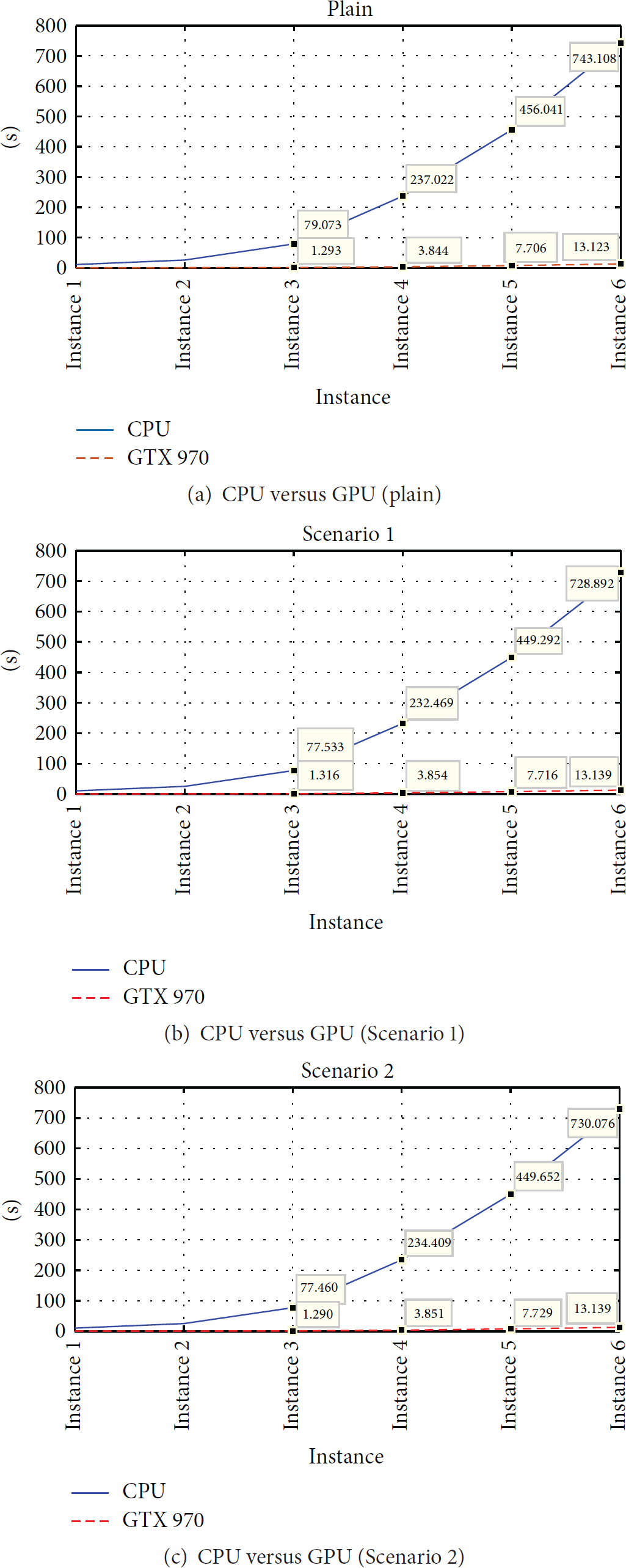
Comparison of CPU and GPU computing time according to scenarios and the number of sensors.

Figure 14

Comparison of computing time between NVIDIA GeForce GPUs.

Figure 15

An example of convergence results of the sensor deployment.

Figure 16

Computing time according to the number of vehicles.

Figure 17

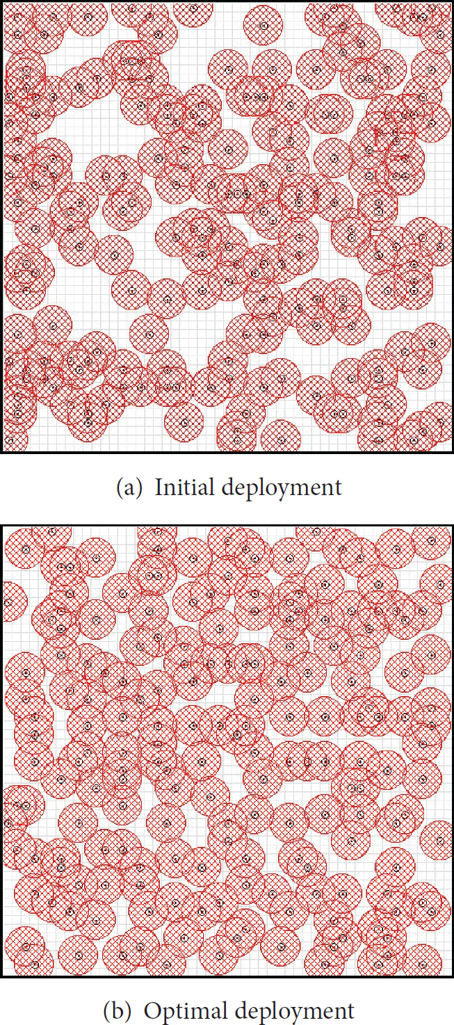
Optimization of sensor deployment on a plain.

Figure 18

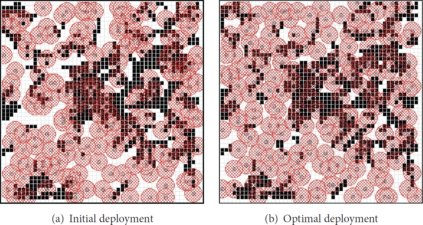
Optimization of sensor deployment on Scenario 1.

Figure 19

Optimization of sensor deployment on Scenario 2.

8. Conclusion

This paper describes the use of a generational GA and probabilistic sensing models in WSN environments to discuss issues relating to barrier coverage. The parts representing the POD calculation and vehicle movements were processed in parallel to improve the efficiency in terms of the computing time when using a generational GA. A comparison of the CPU and GPU experiments showed that the quality of the results of the GPU experiment approximated that of the CPU experiment, while the computing speed became approximately 55-56 times faster. Through experiments in which several GPUs were compared on plains, the GPU specification was analyzed to understand which factors influenced the computing time. In the future, we will use various GA operators, which are convenient for 2D problem solution, for example, [12], and aim to improve the qualities of the solutions. We intend to perform sensor deployment more realistically by taking into consideration factors such as mobile sensors [6], weather impact [28], lifetime, and various deployment methods [29–32] and topographical circumstances, by increasing the parallelization level to enable the computing time to approximate real-time.