Pilot-Less Time Synchronization for OFDM Systems: Application to Power Line Receivers

Abstract

Power line networks provide high-speed broadband communications without the need for new wirings. However, these networks present a hostile environment for high-speed data communications. The most common modulation method used in such systems is OFDM, since it copes effectively with noise, multipath, fading selectivity, and attenuation. A potential drawback of OFDM is its sensitivity to receiver synchronization imperfections, such as timing and sampling frequency offsets. Although several approaches have been proposed for estimating the time and frequency offset, they are based on the use of pilot sequences that are not available in power line communication standards. More importantly, they focus on isolated algorithms for compensating either time or frequency offsets without providing a complete, low complexity, OFDM receiver architecture that mitigates jointly time and frequency errors. This paper focuses on providing an OFDM receiver architecture that can be compatible with many power line standards. Extensive simulation studies show under realistic channel and noise conditions that the proposed receiver provides enhanced robustness to synchronization imperfections as compared to conventional approaches.

1. Introduction

Transmission of data through power line networks has become the preferred connectivity solution to homes and offices [1–3]. Indoor power line networks can offer high-speed data without the need for new wires by using an already-existing infrastructure that is much more pervasive than any other wired system. However, power line networks were originally designed for the transmission and distribution of energy signals at 50 or 60 Hz and as a result they present a hostile environment for high-speed data communications.

A widely adopted method of encoding digital data prior to transmission in power line mediums is the OFDM technique. OFDM ability to cope with severe channel conditions that are present in such networks (e.g., high impulsive noise) has led to its adoption by many industrial consortia for power lines such as the High-Definition Power Line Communication (HDPLC) Alliance [4], the HomePlug Power Line Alliance (HPA) [5], the Universal Power Line Association (UPA) [6], and the ITU-T Gigabit Home Networking (G.hn) [7]. Although it deals effectively with impulsive noise by dividing noise impulses among all the OFDM subcarriers due to the discrete Fourier transform (DFT) operation in the receiver, a potential drawback of OFDM is its sensitivity to receiver synchronization imperfections (e.g., time and sampling frequency errors). Several approaches have been proposed for estimating the time and frequency offset either jointly or individually [8–15].

Specifically, the authors in [8] present a symbol-timing and carrier frequency synchronization method for OFDM systems operating over multipath fading environments. The proposed method uses a specifically designed training sequence, achieving a steep roll-off timing metric trajectory. This type of training symbol achieves some improvement in timing estimation for time-varying multipath Rayleigh fading channels. Also, the work in [9] exploits an interleaved subcarrier-allocation scheme that can be used to fully take advantage of the frequency domain diversity of OFDMA systems. Simulation results also show that the proposed scheme is robust to carrier frequency offset (CFO) estimation errors. However, this approach targets wireless standards and proposes the usage of some extra features that are not employed by the PLC standards. The authors in [10] proposed a solution that deals with CFO estimation by designing OFDM pilot sequences that are periodic in the time domain. The fractional CFO is estimated in closed form by measuring the phase rotations between the repetitive parts of the received preambles, while the integer CFO is estimated in a joint fashion with the MIMO channel matrix by resorting to the Maximum Likelihood (ML) principle. This work is not applicable to a standard that is pilot-less-like [7]. Similarly, the work in [11] incorporates periodic preambles as proposed in wireless standards while pilots are also inserted with a fixed spacing in order to assist the ML Carrier Frequency Offset Estimation Algorithms.

Despite the insights onto the design of isolated algorithms for efficient time and frequency offset estimation and correction in OFDM systems, the aforementioned works are based on the use of pilot sequences that are not available in power line communication standards. The authors in [15] provide a solution for time synchronization that use intrablock phase rotations, achieving significant performance improvements over conventional pilot-assisted estimators relying on interblock phase rotations. In this paper, motivated by the lack of pilot-less schemes for mitigating synchronization imperfection in base band OFDM systems, we propose a complete receiver architecture for broadband PLC systems operating over low and medium voltage networks. The proposed scheme provides a coarse time estimation and mitigation in the time domain using a farrow filter interpolator, followed by a fine estimation at the frequency domain that is based on phase rotations estimated individually for each OFDM symbol. Extensive simulation studies carried out by using a frame format that is adopted in many power line communication standards [4–7] and realistic channel and noise models have shown that the proposed scheme offers robustness against the severe channel and noise conditions that are present in a power line medium, outperforming relevant pilot-less schemes.

The remainder of this paper is organized as follows. In Section 2, we briefly review a baseband OFDM system and the PHY frame structure adopted in PLC standards. In Section 3, we present the different imperfections introduced due to sampling clock errors and symbol-timing offset errors. In Sections 4 and 5, we present the proposed sampling frequency and time offset estimation and mitigation schemes. In Section 6, the performance of the proposed method is evaluated through extensive simulation by selecting parameters in line with power line communication standards. Finally, Section 7 presents a discussion related to prospective difficulties for hardware implementation and Section 8 concludes the paper.

2. OFDM Signal Model and Preliminaries

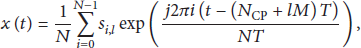
Let us initially consider an OFDM system with N subcarriers as shown in Figure 2. Let

$$\begin{array}{cc}& {\mathbf{s}}_l={\left[\begin{array}{ccc}{s}_{\mathrm{1},l}& \cdots & s_{N,l}\end{array}\right]}^T\end{array}$$

(1)

be a set of N time domain symbols $s_{i,l}$ at the output of the Constellation Mapper which are forwarded at the input of the inverse discrete Fourier transform (IDFT) unit, where l denotes the OFDM symbol time index and i denotes the subcarrier frequency index. The output of the inverse DFT unit may be written as

$$\begin{array}{cc}& {\mathbf{u}}_l={\mathbf{F}}_N^H{\mathbf{s}}_l,\end{array}$$

(2)

where ${\mathbf{F}}_N$ is the normalized $N\times N$ IDFT matrix with elements

$$\begin{array}{cc}& {\left[{\mathbf{F}}_N\right]}_{k,l}=\frac{\mathrm{1}}{\sqrt{N}}{w}_n^{\left(k-\mathrm{1}\right)\left(l-\mathrm{1}\right)},\hspace{1em}k,l=\mathrm{0},\dots ,N-\mathrm{1},\end{array}$$

(3)

with $w_n=e^{-j\left(\mathrm{2}\pi /N\right)}$ and $k,l$ denoting the row and column numbers. The lth OFDM symbol ${\mathbf{u}}_l$ is forwarded at the CP Adder, where the time domain OFDM symbol ${\widehat{\mathbf{u}}}_l$ of length $M=N+N_{\mathrm{C}\mathrm{P}}$ and duration $T_s$ sec is formed by adding a CP of length $N_{\mathrm{C}\mathrm{P}}$ at the beginning of vector ${\mathbf{s}}_l$ . This operation may be described in matrix form as follows:

$$\begin{array}{cc}& {\mathbf{x}}_l={\mathbf{A}}_{\mathrm{C}\mathrm{P}}{\mathbf{u}}_l=\left[\begin{array}{c}\begin{array}{cc}{\mathbf{0}}_{\left(N-N_{\mathrm{C}\mathrm{P}}\right)\times N}& {\mathbf{I}}_{N_{\mathrm{C}\mathrm{P}}}\end{array}\\ {\mathbf{I}}_N\end{array}\right]{\mathbf{u}}_l.\end{array}$$

(4)

The $M\times \mathrm{1}$ OFDM symbol ${\mathbf{x}}_l$ is windowed overlapped and added with the two adjacent $l-\mathrm{1}$ , $l+\mathrm{1}$ OFDM symbols, interpolated, and digitally upconverted by half the signals spectrum, so that all signal energy lies in the positive part of the spectrum. We will use the term upshifting to address this digital IF upconversion from here on.

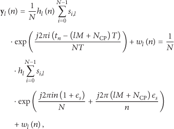
In the receiver side, under the assumption that there is no sampling frequency offset, the baseband signal undergoes digital IF downconversion, a procedure from here on addressed as downshifting and then downsampled at a rate $T=T_s/M$ . We assume that in discrete time model the channel is composed of $L+\mathrm{1}$ independent multipath components, each of which has a gain $h_k$ and delay $k\times T$ , $k=\mathrm{0},\dots ,L$ . The channel taps are assumed to be constant over one OFDM symbol and the received lth OFDM time domain symbol may be written in matrix form as

$$\begin{array}{cc}& {\mathbf{y}}_l={\mathbf{H}}_l{\mathbf{x}}_l+\mathbf{w},\end{array}$$

(5)

where ${\mathbf{H}}_l$ is an $M\times M$ toeplitz matrix with $h_{\mathrm{0}}$ on the main diagonal and $h_{\mathrm{1}},\dots ,h_L$ on the subdiagonals and w is the noise vector. Further details related to the power line channel and noise models are provided in the section that follows.

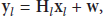
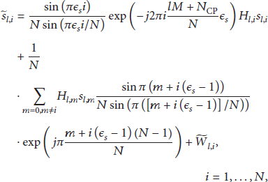
Assuming that we have perfect knowledge of the boundaries of each OFDM symbol in the payload frame section, the lth block of time domain samples ${\mathbf{y}}_l$ passes through the CP removal unit of the OFDM demodulator, where the first $N_{\mathrm{C}\mathrm{P}}$ samples are discarded. This operation may be written in matrix form as

$$\begin{array}{cc}& {\mathbf{z}}_l={\mathbf{R}}_{\mathrm{C}\mathrm{P}}{\mathbf{y}}_l=\left[\begin{array}{cc}{\mathbf{0}}_{N\times N_{\mathrm{C}\mathrm{P}}}& {\mathbf{I}}_N\end{array}\right]{\mathbf{y}}_l,\end{array}$$

(6)

where ${\mathbf{z}}_l=\left[z_{l,\mathrm{1}},\dots ,z_{l,N}\right]$ and $z_{l,i}$ correspond to samples obtained by sampling at time indices $t_{l,i}=\left(i+N_{\mathrm{C}\mathrm{P}}+l\times N\right)T$ . Then, vector ${\mathbf{z}}_l$ passes through the DFT unit whose output reads as

$$\begin{array}{cc}& {\mathbf{r}}_l={\mathbf{F}}_N{\mathbf{z}}_l=\underset{{{\mathbf{H}}_{\mathbf{d}}}_l}{\underbrace{{\mathbf{F}}_N{\mathbf{R}}_{\mathrm{C}\mathrm{P}}{\mathbf{H}}_l{\mathbf{A}}_{\mathrm{C}\mathrm{P}}{\mathbf{F}}_N^H}}{\mathbf{s}}_l+\tilde{\mathbf{w}}={{\mathbf{H}}_{\mathbf{d}}}_l{\mathbf{s}}_l+\tilde{\mathbf{w}},\end{array}$$

(7)

where the entries of $\tilde{\mathbf{w}}={\mathbf{F}}_N\mathbf{w}$ correspond to the frequency domain (FD) representation of noise. Unlike most other communication channels, noise in the power line channel cannot be described by the classical approach of additive white Gaussian noise (AWGN). The following section provides details related to the adopted models for simulating several effects caused by power line channel and noise characteristics [16, 17].

The matrix ${{\mathbf{H}}_{\mathbf{d}}}_l$ is a diagonal matrix with the channel frequency response in the main diagonal:

$$\begin{array}{cc}& {{\mathbf{H}}_{\mathbf{d}}}_l=\mathrm{diag}\left\{\left[H_{\mathrm{0}},\dots ,H_{N-\mathrm{1}}\right]\right\},\\ H_i={\displaystyle \sum }_{k=\mathrm{0}}^L{h}_k{e}^{-\mathrm{2}\pi \sqrt{-\mathrm{1}}ki/N}.\end{array}$$

(8)

The aforementioned diagonalization directly occurs from the fact that ${\mathbf{R}}_{\mathrm{C}\mathrm{P}}{\mathbf{H}}_l{\mathbf{A}}_{\mathrm{C}\mathrm{P}}$ has a circulant structure, and therefore equalization is possible with $\mathcal{O}(N)$ operations.

2.1. Power Line Channel and Noise Model

2.1.1. Channel Model

The channel frequency (impulse) response models the (i) attenuation that is the loss of the power of the signal during its propagation and it depends on the physical length of the channel and the transmission frequency band, (ii) multipath and reflection effects that are caused by the impedance mismatches and mostly dependent on both the physical characteristics and the physical topology of the channel, and (iii) crosstalk between adjacent wires due to electromagnetic coupling. The statistical description of in-home power line channel is based on the work performed in [18], where channel measurements have been conducted in the 0 to 100 MHz range. In particular, it has been shown that the power delay profile has a statistical distribution that could be well described by Weibull and Gaussian distributions.

2.1.2. Noise Model

The additive noise in broadband power line communication channels can be separated into five classes according to Figure 1:

• (i)

Colored noise that results mainly from the summation of harmonics of mains cycle and different low power noise sources present in the system. It has a relatively low power spectral density (PSD), varying with frequency and over time in terms of minutes or even hours.

(ii)

Narrow-band noise that is mostly sinusoidal signals, with modulated amplitudes. This type of noise is mainly caused by ingress of broadcast stations in the long, medium, and short wave broadcast bands. The received level is generally varying during daytime.

(iii)

Impulsive noise that is generated mostly by electrical appliances plugged into the power line network and is classified to (i) periodic impulsive noise synchronous with the AC cycle and (ii) periodic impulsive noise asynchronous with the AC cycle and nonperiodic impulsive noise.

The coloured, narrow-band, and periodic impulsive asynchronous with the AC cycle noise types usually remain stationary over periods of seconds and minutes or sometimes even for hours and may be summarized as background noise. The periodic impulsive noise synchronous with the AC cycle and the nonperiodic impulsive noises are time variant in terms of microseconds and milliseconds. During the occurrence of such impulses the PSD of the noise is perceptibly higher and may cause bit or burst errors in data transmission.

Figure 1

Power line channel model.

Figure 2

Block diagram of an OFDM tarnsmitter.

(i) Color Background Noise Model. According to [18], it can be described by the background power noise density A (dBm/Hz) via the following equation:

$$\begin{array}{cc}& A\left(f\right)=A_{\infty }+A_{\mathrm{0}}{e}^{-f/f_{\mathrm{0}}},\end{array}$$

(9)

where $A_{\infty }$ is the power density for $f\to \infty$ and $A_{\mathrm{0}}$ is the differences between $A_{\infty }$ and $A_{\mathrm{0}}$ . $A_{\mathrm{0}}$ follows a normal distribution, $A_{\infty }$ follows uniform distribution, and $f_{\mathrm{0}}$ is modeled by a shifted exponential distribution with parameters that are defined in [19].

(ii) Narrow-Band Noise Model. The narrow-band interference noise can be modeled as a sum of N multiple sine noise with different amplitudes (deterministic model):

$$\begin{array}{cc}& A\left(t\right)={\displaystyle \sum }_{i=\mathrm{1}}^N{A}_i\left(t\right)\sin \left(\mathrm{2}\pi f_{i}t+{\varphi }_i\right),\end{array}$$

(10)

where N is a number of waves of different frequencies $f_i$ , amplitudes, and phases. The amplitude $A_i\left(t\right)$ is a constant in the simplest case but it can be considered as amplitude modulated for better approximation of AM-broadcast signals. The phase ${\varphi }_i$ is randomly selected from interval $[\mathrm{0,2}\pi ]$ and is not depending on time. The carrier may either be separately synthesized in the time domain or jointly in the frequency domain with help of an IFFT. Further details related to the selection of the aforementioned parameters based on the distances of the radio stations may be found in [18].

(iii) Impulsive Noise Model. To simulate the impulsive noise for the PLC channel we used the Middleton Class A Noise (AWCN) model. The probability density function (PDF) of the real and imaginary part of the complex noise according to this model are approximated by

$$\begin{array}{cc}& p_z\left(z\right)={\displaystyle \sum }_{m=\mathrm{1}}^{\mathrm{3}}\frac{e^{-A}{A}^m}{m!}\frac{e^{{\left|z\right|}^{\mathrm{2}}}/\mathrm{2}{\sigma }_m^{\mathrm{2}}}{\mathrm{2}\pi {\sigma }_m^{\mathrm{2}}}\end{array}$$

(11)

with

$$\begin{array}{cc}& {\sigma }_m^{\mathrm{2}}={\sigma }^{\mathrm{2}}\left(\frac{m/A+\Gamma }{\mathrm{1}+\Gamma }\right),\end{array}$$

(12)

where A is the impulsive index which measures the average number of impulses over the signal period and

$$\begin{array}{cc}& \Gamma =\frac{{\sigma }_g^{\mathrm{2}}}{{\sigma }_i^{\mathrm{2}}}\end{array}$$

(13)

is the Gaussian to impulsive power-ratio (GIR) with Gaussian noise variance ${\sigma }_g^{\mathrm{2}}$ , impulsive noise power ${\sigma }_i^{\mathrm{2}}$ , and total variance ${\sigma }^{\mathrm{2}}={\sigma }_g^{\mathrm{2}}+{\sigma }_i^{\mathrm{2}}$ .

2.2. PHY Frame Structure

The format of the PHY frame is presented in Figure 3. The PHY frame usually includes a preamble, a header, and a payload. The preamble is intended to assist the receiver in detecting, synchronizing to the frame boundaries, and acquiring the physical layer parameters such as channel estimation and OFDM symbol alignment. The preamble consists of a small number of sections as shown in Figure 3. Each section comprises $K_i$ repetitions of an OFDM symbol employing subcarrier spacing $K_i\times f_{\mathrm{s}\mathrm{c}}$ , where $f_{\mathrm{s}\mathrm{c}}$ denotes the subcarrier spacing of the payload symbols and $K_i$ is usually a small integer value. The number of repetitions ( $K_i$ ) and the size of each OFDM symbol $S_i$ ( $N_{S_i}$ samples) in the preamble may change from section to section.

Figure 3

PHY frame structure in time domain.

3. Synchronization Imperfections

In this work we focus only on baseband systems and thus we assume that there is no RF modulator/demodulator. The transmitter baseband part includes inverse discrete Fourier transform (IDFT), CP, windowing, and frequency upshift (see Figure 1). The following considerations motivate us to study the functionalities at an OFDM receiver, in the presence of sampling clock errors and symbol-timing offset errors (we ignore completely carrier frequency offsets since we assume that there is no RF modulator and demodulator at the transceiver and receiver, resp.) which have to be estimated and compensated. More specifically, we assume that (i) the sampling time at the receiver $T^{\prime }$ is not identical to the transmitter sampling time T and (ii) the frame boundaries (i.e., when each preamble section starts and as a result the start of the payload OFDM symbols) are unknown at the receiver. Therefore, the part of the receiver controlling the removal of the CP interval from each payload symbol will usually be offset from its ideal setting by a time $ϵT$ . The received samples at the output of the DFT unit at the receiver that occur by sampling at time indices $t_{l,i}^{\prime }=\left(i+N_{\mathrm{C}\mathrm{P}}+l\times N\right)T^{\prime }$ will be denoted by ${\tilde{\mathbf{r}}}_l$ .

To be able to demodulate efficiently the transmitted signal, we need (i) initially to estimate some flag indicating the first symbol of the frame, the first symbol of each preamble section, and the first symbol of the payload section (frame boundaries) and (ii) then estimate and mitigate the frequency offset due to the inaccuracies of the transmitter and receiver oscillators. The incorporation of the error effects to the time domain baseband model at the output of the frame detector will be the basis for optimizing the receiver components in the following section.

3.1. Frame Boundaries Detection

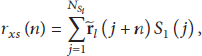
For the detection of frame arrival at the receiver, the received signal is correlated with itself with a delay of one short symbol, given by

$$\begin{array}{cc}& r_{xx}\left(n\right)={\displaystyle \sum }_{j=\mathrm{1}}^{N_{S_i}}{\tilde{\mathbf{r}}}_l\left(j+n\right){\tilde{\mathbf{r}}}_l\left(j+n+N_{S_i}\right),\end{array}$$

(14)

where x denotes the received signal in the time domain, $r_{xx}\left(n\right)$ is the correlation output at the time index n, and $N_{S_i}$ is the length of the short symbol. To smooth the output curve of the autocorrelation process described above, a moving average filter may be also used. The incoming frame can be detected by comparing the magnitude of autocorrelation result at time index n with a specific threshold. In order to be able to detect the preamble section boundaries, we make use of a combination of the aforementioned autocorrelator and the following cross-correlator:

$$\begin{array}{cc}& r_{xs}\left(n\right)={\displaystyle \sum }_{j=\mathrm{1}}^{N_{S_i}}{\tilde{\mathbf{r}}}_l\left(j+n\right)S_{\mathrm{1}}\left(j\right),\end{array}$$

(15)

where $S_{\mathrm{1}}=\left[s_{\mathrm{1}},\dots ,s_{N_{S_{\mathrm{1}}}}\right]$ denotes a preamble short OFDM symbol in time domain. For the detection of the preamble transition we detect a cross-correlation peak combined with a change in the sign of the autocorrelator. Figures 4 and 5 provide the theoretical and practical output of the procedure described above.

Figure 4

Execution example of frame boundaries detector.

Figure 5

Illustration of $r_{xx}$ versus n and $r_{xs}$ versus n.

3.2. Effects of Timing and Sampling Frequency Offset

The receiver OFDM symbol window controlling the removal of the guard interval will usually deviate from its ideal setting introducing a specific timing offset that needs to be estimated and removed. In addition, a sampling frequency offset is also introduced primarily because of the tolerances of quartz oscillators with respect to temperature variations. In the presence of a fixed sampling frequency error the effects that arise after the DFT unit at the receiver are (i) an amplitude reduction, (ii) a phase shift of each QAM symbol $s_{\mathrm{1},i}$ , and (iii) intercarrier interference (ICI) due to loss of orthogonality between the subcarriers. The transmitted baseband OFDM signal can be described as

$$\begin{array}{cc}& x\left(t\right)=\frac{\mathrm{1}}{N}{\displaystyle \sum }_{i=\mathrm{0}}^{N-\mathrm{1}}{s}_{i,l}\exp \left(\frac{j\mathrm{2}\pi i\left(t-\left(N_{\mathrm{C}\mathrm{P}}+lM\right)T\right)}{NT}\right),\end{array}$$

(16)

where l is the OFDM symbol, k is the subcarrier index, T is the sample duration, N is the FFT size, and $N_{\mathrm{C}\mathrm{P}}$ and $M=N+N_{\mathrm{C}\mathrm{P}}$ are the guard interval length and the OFDM symbol length, respectively. With the relative sampling frequency offset (SFO) ${ϵ}_s=(T^{\prime }-T)/T^{\prime }$ the received time domain signal may be written as in [8]:

$$\begin{array}{cc}& {\mathit{y}}_l\left(n\right)=\frac{\mathrm{1}}{N}{h}_l\left(n\right){\displaystyle \sum }_{i=\mathrm{0}}^{N-\mathrm{1}}{s}_{i,l}\exp \left(\frac{j\mathrm{2}\pi i\left(t_n-\left(lM+N_{\mathrm{C}\mathrm{P}}\right)T\right)}{NT}\right)+w_l\left(n\right)=\frac{\mathrm{1}}{N}{h}_l{\displaystyle \sum }_{i=\mathrm{0}}^{N-\mathrm{1}}{s}_{i,l}\exp \left(\frac{j\mathrm{2}\pi in\left(\mathrm{1}+{ϵ}_s\right)}{N}+\frac{j\mathrm{2}\pi \left(lM+N_{\mathrm{C}\mathrm{P}}\right){ϵ}_s}{n}\right)+w_l\left(n\right),\end{array}$$

(17)

where $t_n=\left(lM+N_{\mathrm{C}\mathrm{P}}\right)T^{\prime }+n{T}^{\prime }$ and $w_l(n)$ is samples of noise. After FFT the frequency domain samples at the receiver side becomes

$$\begin{array}{cc}& {\tilde{s}}_{l,i}=\frac{\sin \left(\pi {ϵ}_{s}i\right)}{N\sin \left(\pi {ϵ}_{s}i/N\right)}\exp \left(-j\mathrm{2}\pi i\frac{lM+N_{\mathrm{C}\mathrm{P}}}{N}{ϵ}_s\right)H_{l,i}{s}_{l,i}+\frac{\mathrm{1}}{N}{\displaystyle \sum }_{m=\mathrm{0},m\ne i}{H}_{l,m}{s}_{l,m}\frac{\sin \pi \left(m+i\left({ϵ}_s-\mathrm{1}\right)\right)}{N\sin \left(\pi \left(\left[m+i\left({ϵ}_s-\mathrm{1}\right)\right]/N\right)\right)}\exp \left(j\pi \frac{m+i\left({ϵ}_s-\mathrm{1}\right)\left(N-\mathrm{1}\right)}{N}\right)+{\tilde{W}}_{l,i},\hspace{1em}i=\mathrm{1},\dots ,N,\end{array}$$

(18)

where ${\tilde{W}}_{l,i}$ is the frequency domain samples of noise and $H_{l,m}$ is the channel frequency response at the mth frequency bin and $\sin \left(\pi i{ϵ}_s\right)/N\sin \left(\pi i{ϵ}_s/N\right)\cong \mathrm{1}$ .  

4. Sampling Frequency Offset Estimation and Mitigation at Time Domain

In this section we will give a brief description of the methods applied for estimating and mitigating the effects of the difference between the sampling period $T^{\prime }$ at the receiver and T at the transmitter, leading to a relative sampling frequency error ${ϵ}_s=(T^{\prime }-T)/T^{\prime }$ , so called sampling frequency offset.

4.1. SFO Acquisition

Initially, the estimation of the sampling frequency offset denoted by ${ϵ}_s$ can be performed by exploiting the structure of the preamble and comparing the phases between successive repeated symbols on all the frequency bins at the FD. The phase difference between the FFT values of the successive received preamble symbols has two main causes [9]: (i) either carrier frequency offset or (ii) sampling frequency offset. Since we have assumed that there is no carrier frequency offset, the phase difference is exclusively attributed to SFO. At this point it should be pointed out that in the PLC case, the accuracy of applying the conventional FFT and estimating the phase difference is significantly reduced, due to the presence of impulsive noise and the fact that the power signal contains multiple harmonics.

To overcome this limitation, a special FFT algorithm, so called all phase FFT (APFFT), [20] is often employed. According to this algorithm, a vector that consisted of two repeated known symbols is initially formed:

$$\begin{array}{cc}& {\mathbf{r}}_{l\mid l+\mathrm{1}}=\left[r_{l,\mathrm{1}},\dots ,r_{l,N}\mid r_{l+\mathrm{1,1}},\dots ,r_{l+\mathrm{1},N}\right].\end{array}$$

(19)

Then, the ouput is computed as

$$\begin{array}{cc}& {\mathcal{R}}_l={\mathbf{F}}_N\left[{\mathbf{C}}_{\text{:},\mathrm{1}}+{\mathbf{C}}_{\text{:},\mathrm{2}}+\cdots +{\mathbf{C}}_{\text{:},N}\right],\end{array}$$

(20)

where ${\mathit{C}}_{:,i}$ denotes the i column of the circulant matrix C with ${\mathbf{C}}_{:,\mathrm{1}}={\left[r_{l+\mathrm{1,1}},r_{l,N},\dots ,r_{\mathrm{2},N}\right]}^T$ .

Similarly, from symbols ${\mathbf{r}}_{l+\mathrm{1}\mid l+\mathrm{2}}$ we are able to calculate ${\mathcal{R}}_{l+\mathrm{1}}$ and it can be easily shown that

$$\begin{array}{cc}& {\mathcal{R}}_{l+\mathrm{1}}\left(i\right)={\mathcal{R}}_l\left(i\right)e^{-\mathrm{2}\sqrt{-\mathrm{1}}\pi {ϵ}_{s}i}.\end{array}$$

(21)

The SFO ${ϵ}_s$ can then be estimated from the ith APFFT output of consecutive symbols that are spaced N samples apart, as follows:

$$\begin{array}{cc}& \widetilde{{ϵ}_{s_i}}=\frac{\mathrm{1}}{\mathrm{2}\pi i}\angle \frac{{\mathcal{R}}_l\left(i\right)}{{\mathcal{R}}_{l+\mathrm{1}}\left(i\right)}.\end{array}$$

(22)

At this point it should be noted that in practice the repeated symbols of the 1st preamble section have length $N_s<N$ . In order to reduce the complexity of the aforementioned estimator an APFFT unit of length $L_s<N_s$ could be employed. In that case (22) may be rewritten as

$$\begin{array}{cc}& \widetilde{{ϵ}_{s_i}}=\frac{N_s}{\mathrm{2}\pi i{L}_s}\angle \frac{{\mathcal{R}}_l\left(i\right)}{{\mathcal{R}}_{l+\mathrm{1}}\left(i\right)}.\end{array}$$

(23)

To efficiently exploit the estimation based on each output i of the APFFT unit a least square estimator may be used (LS Fit unit in Figure 6(c)). The output of this estimator can be written as

$$\begin{array}{cc}& \widetilde{{ϵ}_s}={\left({\mathbf{f}}^T\mathbf{f}+\delta \right)}^{-\mathrm{1}}{\mathbf{f}}^T\varphi ,\end{array}$$

(24)

where $\mathbf{f}={\left[\mathrm{0,2}\pi L_s/N_s,\dots ,\mathrm{2}\pi L_s(N_s-\mathrm{1})/N_s\right]}^T$ , $\varphi =\left[{\varphi }_{\mathrm{0}},\dots ,{\varphi }_{N_s-\mathrm{1}}\right]$ , ${\varphi }_i=\angle {\mathcal{R}}_l(i)/{\mathcal{R}}_{l+\mathrm{1}}(i)$ , and δ is a samll constant (i.e., $\delta =\mathrm{1}{\mathrm{0}}^{-\mathrm{4}}$ ).

Figure 6

Block diagram of an OFDM receiver, robust to timing and sampling frequency errors.

Similarly to the initial SFO estimation process, tracking of the SFO variations can be performed in a similar way by autocorrelating the APFFT outputs of consecutive CPs that are spaced L samples apart. The measured slope of the phase differences (including phase difference and time filtering) will provide the SFO estimation. A block diagram of the operations described above is given in Figure 6(c).

4.2. Farrow Sample Rate Converter (SRC)

This unit evaluates the new sample values at arbitrary points between the existing samples by utilizing a digital interpolation filter. The input sequence $\dots ,x(\left(n_l\mathrm{2}\right)T^{\prime }),x(\left(n_l\mathrm{1}\right)T^{\prime }),x(n_l{T}^{\prime }),x(\left(n_l+\mathrm{1}\right)T^{\prime }),x(\left(n_l+\mathrm{2}\right)T^{\prime }),\dots$ is formed of the uniformly spaced samples with respect to the sampling interval $T^{\prime }$ . The new sample $y(lT)$ , also called the interpolant, occurs between the samples $x(n_{l}Tx)$ and $x((n_l+\mathrm{1})Tx)$ , at the point $lT=n_l{T}^{\prime }+{\mu }_l{T}^{\prime }$ , where $n_l$ is the basepoint index and ${\mu }_l$ is the fractional interval. The fractional interval can take any value in the range $\mathrm{0}\le {\mu }_l<\mathrm{1}$ . An efficient implementation of a lagrange polynomial interpolation filter can be realized by using a farrow structure [21] as the one shown in Figure 6(d).

5. Time Offest Estimation and Mitigation at Frequency Domain

Sampling timing offset (STO), significantly downgrades the system performance and is attributed to the fact that the equalizer (EQ) coefficients estimated by the probe frame are outdated. To be compatible with the power line standards, we choose to estimate the equalizer coefficients by exploiting the presence of a probe frame (PROBE CE EQcoeffs) which are transmitted between the data frames. Ideally, if channel estimation and equalization were performed at each frame, then we would not suffer from any STO issues. However, in a real life scenario, we need to compensate the STO, by appropriately adjusting the phase of the equalizer coefficients that are going to be applied in each frame. The referenced coefficients for STO estimation are the EQ coefficients estimated from the preamble section (Preamble CE EQ). To be more specific, we initially estimate the phase shift between the corresponding coefficients of the Preamble CE EQ and the PROBE CE EQcoeffs. Motivated by the fact that the resulting shifts correspond to a series of values that can be fitted by a line, we choose to estimate the line parameters (e.g., slope and offset) by using a least square (LSfit) procedure similar to that presented in (24). The estimated slope corresponds to the STO, while the offset value is caused mainly by the mismatch between the phase shifts of the RX downshifter and the TX upshifter, due to their free-running nature. After deriving these parameters, we compensate the phase of each PROBE CE EQ coefficient by performing a simple fixed point multiplication of the stored EQ coefficient with a value that corresponds to the phase mismatch between the preamble and probe coefficients. In hardware, this operation is efficiently implemented by using a cordic rotation [22]. At this point, it should be also mentioned that during the LSfit procedure, we need to take also into account the subcarrier masking (SM) values defined by the corresponding standard.

6. Performance Evaluation

We have developed a MATLAB simulator that incorporates both the transmitter and receiver blocks presented in Figures 2 and 6, while the channel and noise have been modeled accordingly. In order to introduce a sampling frequency offset we have used the farrow structure described above. Integer STO is caused by frame boundary detection errors; that is, the start of the frame flag raised some samples earlier or later. Finally, to introduce fractional STO we took advantage of the interpolation unit at the transmitter. By starting our sample collection at the receiver from any of the available interpolation factor samples that correspond to a noninterpolated sample we can simulate fractional STO with a step quantized to 1/interpolation factor. We have considered the channel and noise models presented in Section 2. For the AWCN noise the GIR ratio was set to 0.05.

In the following subsection, we present the results of our experiments. The PHY layer parameters are presented in Table 1. A sampling frequency offset equal to 40 ppm and a timing offset of 1.3 samples were introduced.

Table 1

System parameters.

Parameter	Value
OFDM Payload Symbol Length (N)	2048
Cyclic Prefix Length ( $N_{\mathrm{C}\mathrm{P}}$ )	512
Window Value β	256
Interpolation factor	10
Sampling frequency offset values	40 ppm
Timing offset values	−1.3 samples
Constellation	QAM 64
OFDM Preamble Symbol Length ( $N_{S_1}$ )	256
Number of preamble sections	7 + 2
Bandplan	50 MHz
Payload Subcarrier Spacing	24.4140625 kHz
Preamble Subcarrier Spacing	195.3205 kHz

In Figure 7 we plot the Constellation diagrams for the fifth payload OFDM symbol at (a) the output of the equalizer, (b) the output of the phase corrector with the decision directed phase tracker deactivated, where it is clearly shown that phase distortion due to residual SFO is evident, and (c) the output of the phase corrector with the decision directed phase tracker activated, where residual SFO has been compensated. Any phase corruption is mitigated when both SFO corrector and phase tracker are enabled.

Figure 7

Scatterplot of equalized symbols with (a) farrow SRC and phase corrector disabled, (b) farrow SRC enabled and phase corrector disabled, and (c) farrow SRC enabled and phase corrector enabled.

In Figure 8 we provide the phase shift between the received and the original OFDM symbols measured at each subcarrier at the output of the receiver DSP blocks. More specifically, we plot the phase shifts (a) at the output of the equalizer, before the phase corrector, (b) at the output of the phase corrector with the decision directed phase tracker deactivated, and (c) at the output of the phase corrector with the decision directed phase tracker activated. When the phase tracker is deactivated (case b) the effect of residual SFO is demonstrated, with the phase slope increasing with the count of OFDM symbols. At this point, it should also be noted that the phase tracker measurement period is two OFDM symbols hence OFDM symbols 3 and 5 have the best phase error compensation.

Figure 8

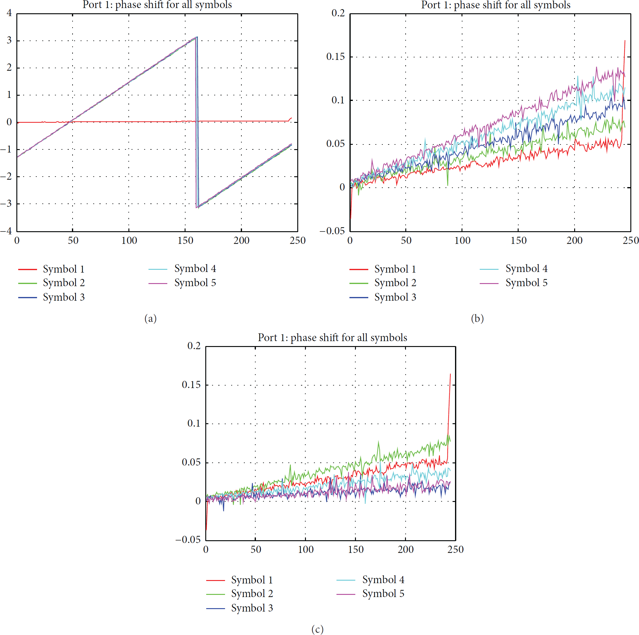
These plots are taken from probe symbols in the frequency domain only, that is, (a) equalizer output, (b) rotator output (phase tracker off), and (c) rotator output (phase tracker on). Farrow SRC is always on.

Finally, we performed an extensive evaluation by enabling and disabling the farrow filter. We assumed 16 QAM symbol. The STO was set to 0.124 samples and the SFO at 200 ppm, while we transmitted in total ${\mathrm{10}}^{\mathrm{6}}$ symbols. In Figure 9 we provide the measured mean square error at the output of the QAM demapper for different measured SNR values at the receiver.

Figure 9

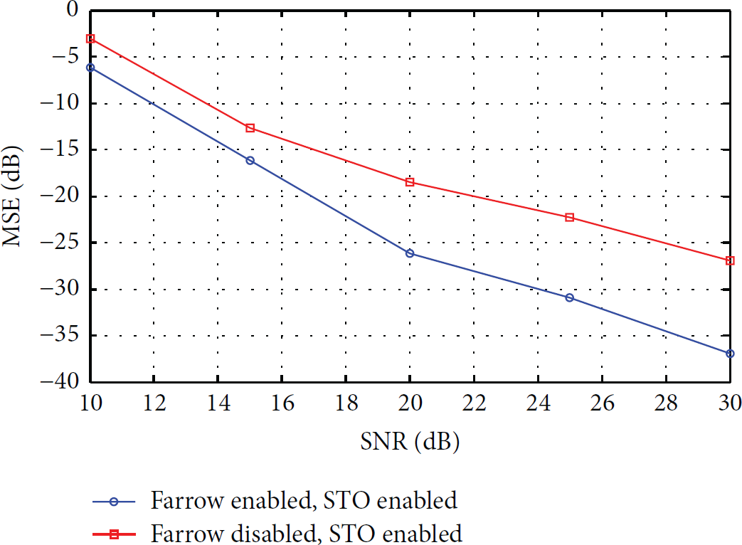
MSE versus SNR with and without the farrow interpolator.

At this point it should be noted that the Gaussian to impulsive noise ratio was set to 0.05. By inspecting Figure 9 it can be shown that the use of the sample rate converter at the time domain significantly increases the robustness of the system in a PLC environment. Motivated by this remark we expect that the use of a farrow interpolator at the TD could be beneficial for other similar methods that consider both SFO and STO and perform only phase rotation after the FFT unit at the demodulator side (e.g., [15]).

7. Discussions

7.1. Impulsive Noise Modeling

In most cases the structure of the impulses induced in PLC channels consist of damped sinusoids, while the most powerful contents of these impulses are located in low frequencies and are represented as the sum of damped sinusoids:

$$\begin{array}{cc}& n_i\left(t\right)={\displaystyle \sum }_{k=\mathrm{1}}^{N_d}{A}_k\sin \left(\mathrm{2}\pi f_k\left(t-t_p\right)+{\varphi }_k\right)e^{\left(-t-t_p\right)/t_k}\eta \left(\frac{t-t_p}{t_n}\right),\end{array}$$

(25)

where $N_d$ is the number of damped sinusoids that form the impulse, $A_k$ , $f_k$ , and ${\varphi }_k$ represent the amplitude, the frequency, and the phase of the kth sinusoid, $t_p$ is the arrival time of the impulses, k is the damping factor, and $\eta (t)$ denotes a square pulse with a duration of $t_n$ . The amplitude of each damped sinusoid $A_k$ is selected to be $~N\left(\mathrm{0},G_k{\sigma }_n^{\mathrm{2}}\right)$ , where $G_k$ denotes the increment of the impulse over the background noise with a variance of ${\sigma }_n^{\mathrm{2}}$ . Values of $G_k$ can range between 20 and 30 dB.

Alternatively to the aforementioned model the AWCN model can be employed as described in Section 2. With the AWCN model, various classes of impulsive noise are expressed by a simple function with a small number of parameters. However, the disadvantage of this model is the fact that it does not define time domain features. The PDF does not describe whether the noise waveform is peaky (impulsive) or smooth in the time domain. This is because the noise of the proposed model has different variances at different phases of the AC voltage. In other words, the Middleton PDF in PLC channel is the description of power line noise without the consideration of time depending (periodic) features. Thus with the stationary model we can define the time arrival and duration of impulses, while with the Middleton model we can simulate random spikes that arrive at random time intervals.

7.2. Prospective Difficulties for Hardware Implementation

The digital implementation of a power line OFDM baseband modem is in itself a difficult procedure. Due to the resources limitations and the demand for low power of the hardware platforms used in sensor network infrastructures, the design team should proceed with a systematic trade-off analysis between OFDM performance and the usage of specific fixed point arithmetic during the hardware development. This trade-off analysis will also have an impact to the cost of the sensor network fabrication. The difficulty of approaching the best performance of the OFDM systems stems from the fact that the design team (most of the time) should compromise with an affordable performance degradation which will not affect the specified link-budget. Consequently, each parameter used in the OFDM baseband receiver requires retuning taking into account both the power line channel impairments and the specified performance. The algorithms presented in this paper are selected accordingly in order to lead to a straightforward hardware implementation taking into account the potential limitations.

8. Conclusion

OFDM is the most commonly adopted scheme from many power line communication standards. However, its sensitivity to receiver synchronization imperfections motivated researchers to provide isolated solutions for estimating either the time or the sampling frequency offset individually. This paper focuses on providing a complete architecture that can be adopted by low complexity power line receivers for compensating any kind of synchronization errors in power line networks. The proposed solution provides a robust estimation and mitigation of time and frequency imperfections, without making use of pilot symbols that are not present in many existing power line standards.