Sports Motion Recognition Using MCMR Features Based on Interclass Symbolic Distance

Abstract

Human motion and gesture recognition receive much concern in sports field, such as physical education and fitness for all. Although plenty of mature applications appear in sports training using photography, video camera, or professional sensing devices, they are either expensive or inconvenient to carry. MEMS devices would be a wise choice for students and ordinary body builders as they are portable and have many built-in sensors. In fact, recognition of hand gestures is discussed in many studies using inertial sensors based on similarity matching. However, this kind of solution is not accurate enough for human movement recognition and cost much time. In this paper, we discuss motion recognition in sports training using features extracted from distance estimation of different kinds of sensors. To deal with the multivariate motion sequence, we propose a solution that applies Max-Correlation and Min-Redundancy strategy to select features extracted with interclass distance similarity estimation. With this method, we are able to screen out proper features that can distinguish motions in different classes effectively. According to the results of experiment in real world application in dance practice, our solution is quite effective with fair accuracy and low time cost.

1. Introduction

Recognition of human motions and gestures is commonly studied in sports field so as to serve movement analysis, guidance, and evaluation. Since direct observation costs too much human resources, information techniques are introduced to assist the tasks. Video and photography are used to record human movement, and there are quite a lot of researches in analyzing the visual information [1]. For more precise analysis, 3D modeling technology [2, 3] is also used to build 3-dimensional model of movement of human body. These methods provide accurate report of human motions and gestures, but for ordinary students and exercisers, they may not afford such devices. Meanwhile, the application of these visual devices is not convenient due to the restriction of space. As for the development of smart mobile terminals, wearable sensors are popularized in many fields, such as medical and health services [4–6] as well as sports domain [7, 8]. Take running, for instance, we are able to detect the running speed, trajectories, and the calories we burn during the exercises. Most of these sensing data are obtained by microelectromechanical systems (MEMS), which is the technology of very small devices. It merges at the nanoscale into nanoelectromechanical systems (NEMS) and nanotechnology [9]. MEMS sensors can be embedded in smart phone, watch, wristband, and other wearable objects, even clothes and shoes. These sensors are portable and low cost, which is quite acceptable for the public. Therefore, to assist sports training of students, we collect the motion data with MEMS sensors for certain action recognition. Although quite a lot of contributions have been made in this domain, most of them focus on regular activity recognition with repeated motions. Recent studies in gestures recognition usually involve time consuming similarity comparison in testing phase that might be a problem in recognizing long time complex motions.

In this paper, we attempt to find a fast and accurate way to recognize certain sports movements with wearable sensors. Our job includes motion data collection and preprocessing with multiple motion sensors embedded in MEMS; feature extraction and selection; and class determination of the unlabeled data. In this process, we may face the following difficulties and problems:

• (i)

Selection and fusion of multiple sensors.

(ii)

Similarity matching between multivariant motion series.

(iii)

How to improve the efficiency for online detection.

As there is no clear guidance for sensor selection, the choices are various in different studies. Normally, activity recognition would choose more sensors and related statistics to generate different features, while recognition based on distance metric usually chooses few key sensor data obtained after dimensional reduction for the comparison. In our study, we will discuss different situations with single or multiple sensors. Since the data we obtain come from different sensors and DoF, we need to find an effective way to deal with this multidimensional data. Moreover, finding an efficient solution for online motion recognition based on distance metric that considers the mutual distance relationship information will be another important task. As a result, we propose a flexible and interpretable solution using interclass distance features from the mutual distance between testing data and different classes. With Max-Correlation and Min-Redundancy strategy, we choose the nonredundant and distinguishable features and apply them in traditional classifiers. After careful observation of related experiments, we find that DTW based on SAX would be a good trade-off between time and accuracy as the distance metric. This solution is applied in physical education using smart phone to detect and analyze basic movements in dance practice.

The rest of the paper is organized as follows: related works are discussed in Section 2; data collection and basic preprocessing are discussed in Section 3; in Section 4, we describe our solution starting from feature extraction and selection to data classification; discussion of related experiments is arranged in Section 5; and finally comes the conclusion of the study in Section 6.

2. Related Work

Wearable sensors are usually used to detect different activities, hand gestures, and specific motions. Activity recognition [10, 11] is used to distinguish different states of human, such as running, walking, going upstairs, and going downstairs. These states consisted of repeated motions, which is a special characteristic that can be used in pattern recognition. Hand gestures recognition in man-machine interaction is also a hot topic that attracts much attention [12, 13]. Similarity comparison between the obtained data and standard model is a common way to solve the problem. There are also studies that focus on specific movement detection, such as fall [14], smoking [5], and body shaking [15]. In some cases, multiple sensors on different parts of human body would improve the recognition accuracy; thus wearable sensor groups are built to detect human status [16, 17]. At present, beside the body sensor network with different types of sensors on different part of the body that can be used in medical field, cluster of the same type of sensors on different part of human body is mainly discussed in activity and motion analysis. Professional training may prefer high accuracy, and multiple sensors would be a better choice. As for ordinary practice, sensors on a single part of the body would be wiser, considering the trade-off between accuracy, cost, and convenience. Most studies choose acceleration information to judge human state [18], and some of them also take gyroscope and magnetometer into consideration [19]. Sensor fusion is discussed in activity recognition based on feature extraction in time and frequency domains [20]. According to the observation of related experiments, sensor selection and fusion have close relations with the discussed activities, placing position of the sensor, type of the classifier, and the extracted features. It is difficult to make the choice beforehand. Therefore, how to make full use of information from different types of sensors efficiently without redundancy is a significant job to do.

As for motion recognition, there are generally two ways to handle the data. The first one is to extract features in time and frequency domains in each fragment divided by sliding window. And then, perform dimensional reduction on these features. After that, ordinary classifiers can be used to predict motion categories. This method is commonly used in activity recognition that contains repeated motions [21]. In such cases, the probability and statistics information is more efficient and useful. However, in recognizing specific motions such certain sports gestures and movements, the differences between various motion types might exist in shape of certain location. And the statistical features might fail in reflecting these differences. Another solution of motion recognition is based on distance metric. Distances between the testing data and training data can be used to build a k-NN (1-NN + DTW is supposed to be quite effective) classifier for further prediction [22, 23]. But the comparison in the testing phase might take too much time. For some high time cost distance measurements such as DTW, this may affect the efficiency, especially for online motion recognition. Therefore, study in [24] proposed an application of Nearest Centroid Classifier using average series based on DTW [25] as centroids. Also, template matching is quite popular. By directly comparing the testing motion data with a few prototype template generated from different classes called motifs, we are able to tell the type of motion the testing data belongs to. The main idea of the previous related researches focus on finding the optimized samples that can better represent the features of the categories they belong to [26–31]. Some studies also consider the separability between different classes [32].

Motion data can be treated as time series, and there are many related studies around the topic of time series similarity estimation. First of all, we can divide the existing methods into two categories: estimations based on global similarity and local similarity. Solutions belonging to the first category use the global matching cost/distance to be the similarity measurement, while, for data with noise, local similarity may be more accurate. The structure of related works are shown below:

• (i)

Global matching similarity:

• (1)

Similarity based on different distance metric:

• (a)

Dynamic time warping (DTW) [33, 34]:

• (I)

DTW with constraints [35, 36].

(II)

Dynamic Manifold Warping (DMW) [37].

(III)

TWED [38].

(b)

Traditional distance:

• (I)

Manhattan distance.

(II)

Euclidean distance.

(III)

Mahalanobis distance.

(2)

Symbolic based measurement:

• (a)

Edit distance.

(b)

Symbolic Aggregate approximation (SAX) [39].

(ii)

Local matching similarity:

• (1)

Longest Common Subsequence (LCS) [40].

(2)

Similarity based on shapelet [41].

Dynamic time warping (DTW) is most commonly used in real-time generated time series like motion and voice signal. Unlike Euclidean distance, this method tolerates offsets and time shifting during the comparison, which is quite suitable for our situation. But the time consumption of DTW is quite high, and it is one of the challenges we need to deal with. There are many attempts in improving DTW in different aspects. For example, different kinds of constraints are set for comparison, so as to reduce the time consumption [42]. Symbolic comparison is another common way to measure the similarities between time series, such as Edit distance and LCS. These methods are more suitable for symbolic comparison like string matching. As for continuous time series, they need to combine with other methods. For example, TWED use Edit distance to replace Euclidean distance in the matching process of DTW. Before the direct matching, transformation of raw data or related operation should be defined. SAX is a simple method that converts continuous time series into discrete symbolic series. We can also use SAX to compute the lower bound distance efficiently. Meanwhile, the process of discrete symbolic representation is also a special way of dimensional reduction. Direct comparison with one labelled sample from each class is fast and easy, but its accuracy cannot compare with classifiers. In some circumstances, the shape of the time series with noise might be quite similar globally, while local features are various according to different categories. Shapelet was proposed to solve such problem. Shapelet is a subsequence taken from one of the time series, whose distance to different time series can be used to distinguish time series from different categories. In order to work with commonly used classifiers, the solution called shapelet transform [43, 44] was brought up. The distances between a time series and all shapelets are treated as the selected features of the time series that can be handled in all kinds of classifiers.

Most of the existing distance based methods determine the categories of the unlabeled data according to their closest motifs or samples selected by different mechanisms. The guidance information of the classification is limited in the distance between testing data and the nearest model, no matter how superior these prototypes are. Information of the mutual distance relationship between the testing data and different classes is left out. Thus, how to make rational use of the mutual distance between different classes is the key problem we need to solve. In our solution, we consider the information of mutual distance between samples and different classes and use them as features for classification. In this way, we can speed up the recognition while maintaining high accuracy.

3. Data Collection

According to the situation and requirement of motion practice in physical education, we choose sensors embedded in smart phone to obtain the data of movements and gestures. Nowadays a smart phone carries more and more types of sensors, including accelerometer, gyroscope, gravity sensor, and magnetometer. These sensors reflect the status of the phone from different aspects. 3D accelerometer measures the acceleration on three mutual perpendicular directions. This acceleration is affected by gravity, so we need to separate the linear acceleration from the original data. 3D gyroscope obtains the rotation rate on 3 coordinates. Based on the readings of the sensors, we are able to obtain the attitude information of the smart phone. Magnetometer measures magnetic density and direction, so that we can detect the orientation of the smart phone.

In our case, we use iPhone 6 to sense human motion. The system editions after iOS 4 provide us with Core Motion Framework that can read the data of all kinds of sensors and conduct essential preprocessing. Specifically, with the class called CMDeviceMotion, we are able to get information about movement and attitude of the smart phone. This class mainly consists of four parts: attitude information calculated with reading of the embedded sensors; gravity data obtained by accessing gravity sensor; acceleration that has removed the influence of gravity and finished the filtering; rotation rate that has removed the bias of gyroscope. By calculating the reading of the different sensors, attitude of the smart phone is described as a quaternion and three-dimensional Euler angles: yaw, roll, and pitch.

After careful observation and analysis, we decided to wear a packet on the frontal side of the waist and put the smart phone inside the packet with its screen towards the front. We set 20 Hz as the sampling rate. We show some of the data we obtain from motion A in Figure 1: stepping forward and backward in 8 beats.

Figure 1

Some of the data provided by Core Motion Framework: including acceleration after filtering and gravity removal, rotation rate without bias, attitude information such as Euler angles and quaternion obtained from different sensors, and data received by gravity sensor and magnetometer. The sampling rate of the data is 20 Hz.

Since the direction of the phone changes constantly, it is hard to determine the instant state of the phone. One common way to eliminate such influence is to add a dimension: magnitude. As for acceleration in three dimensions, x, y, and z, magnitude is defined in the following:

$$\begin{array}{cc}& \text{magnitude}=\sqrt{x^{\mathrm{2}}+y^{\mathrm{2}}+z^{\mathrm{2}}}.\end{array}$$

(1)

With magnitude, we can ignore the variation of direction at a certain degree, but we fail to see the status on each dimension separately. Thus, we transform the linear acceleration and gyroscope data from coordinates of the phone to Earth coordinates. It is calculated with the equations below

$$\text{lin\_acc\_earth}=R·\left(\text{acc}-\text{grav}\right),$$

(2a)

$$\text{gyro\_earth}=R·\text{gyro}.$$

(2b)

Here, R is the rotation matrix [45].

With data from the readings of each sensor, fusion of different sensors, and coordinates transformation, we finally obtain a 31-dimensional time series that can be arranged in 9 groups. The details are shown in Table 1.

Table 1

Sensor data collection.

Name	Coordinates	Description
accelerometerAcceleration	X, Y, Z	Reading of accelerometer
gyroRotation	X, Y, Z	Reading of gyroscope
Euler Angles	Yaw, roll, and pitch	Rotation attitude
motionRotationRate	X, Y, Z	Reading of gyroscope without bias
motionUserAcceleration	X, Y, Z	Acceleration without gravity
motionQuaternion	X, Y, Z, W	Spatial orientation and attitude
motionGravity	X, Y, Z	Output of gravity sensor
motionMagneticField	X, Y, Z	Magnetometer data
lin_acc_earth	X, Y, Z	Linear acceleration relative to Earth
gyro_earth	X, Y, Z	Gyroscope data relative to Earth

4. Motion Recognition Based on MCMR Interclass Distance Features

The sensor data of each motion is a fragment of unrepeated multivariant time series. For this kind of data, we usually apply methods based on distance similarity. Here, in our study, we are facing the multidimensional data from sensor fusion and the problem of matching efficiency. Inspired by shapelet transform in time series recognition, we use distances to samples from different classes to determine the class label of the testing data. Shapelet transform uses Euclidean distances to be the candidates of features for further classification. However, in our cases, this kind of measurement faces the challenge of data offsets and shifting as well as high data dimension and large time consumption. Therefore, we design a fast DTW measurement based on symbolic representation. To eliminate the influence of noise while speeding up the calculation, we use SAX to transform the original time series into shorter symbolic series before distance estimation. We are not sure what kind of sensor and which dimension is more significant in distinguishing different motions, so we use Max-Correlation and Min-Redundancy strategy to select proper candidates to participate in classification of the next step. The chosen features can be used in all kinds of classifiers. It is flexible enough for us to choose suitable classifiers with good performance according to actual situation. The procedure of the recognition solution is demonstrated in Figure 2.

Figure 2

The procedure of our motion recognition solution: firstly, the motion series are preprocessed by Z-normalization and symbolic representation; secondly, representative sequences are selected from training data as feature candidates using distance transformation; thirdly, features with high distinguish ability and low redundancy are chosen; finally, the selected features can be used to build all kinds classifiers for motion recognition.

Motion time series recognition based on distance metric uses the distances between time series as a kind of dissimilarity measurement and works in many similar situations, such as the NN-embedded distance and similarity measurement between testing samples and selected motifs. Unlike these methods, we try to use distances between testing motion series and sequences from different classes as values of the classification features and apply in different kinds of classifiers. Since various divergences appear in time and range of the same movement performed by different people as well as the same people in different time, we use DTW based method as the distance estimation. Meanwhile, considering the high calculation time, we reduce the dimension of the data using symbolic representation. The details of this solution will be described in the rest of this section.

Before further discussion, we summarize the notations throughout the paper in Abbreviations section.

With the data obtained in Section 3, we have the following definition of our research object.

Definition 1 (motion time series based on sensor fusion).

$S=\{s_{\mathrm{1}},s_{\mathrm{2}},\dots ,s_m\}$ is a multidimensional time series that represents a single movement with m-dimensional sensor data. $s_i=\{s{d}_{\mathrm{1}},s{d}_{\mathrm{2}},\dots ,s{d}_{n_i}\}$ indicates the data in ith $(\mathrm{1}\le i\le m)$ dimension with length $n_i$ .

In our case, m is 31, and n varies for different motions.

4.1. Data Preprocessing and Representation

Since the same motion with similar shapes might be far away from each other due to the difference of the action range. Data normalization is needed to eliminate this divergence. For the time series in ith dimension $s_i$ , its Z- $normalization$ is shown in the following:

$$\begin{array}{cc}& s_{i\_\mathrm{n}\mathrm{o}\mathrm{r}\mathrm{m}}=\frac{s_i-{\mu }_{s_i}}{{\sigma }_{s_i}}.\end{array}$$

(3)

Here, the mean ${\mu }_s$ and standard deviation ${\sigma }_s$ are defined as follows:

$$\begin{array}{cc}& {\mu }_{s_i}=\frac{\sum s{d}_i}{n},\\ {\sigma }_{s_i}=\sqrt{{\displaystyle \sum }_{j=\mathrm{1}}^n\frac{{\left(s{d}_{i_j}-{\mu }_{s_i}\right)}^{\mathrm{2}}}{n}}.\end{array}$$

(4)

In order to reduce the time consumption while eliminating the influence of noises, we transform the continuous time series into discrete symbolic series using SAX. The time series is divided into fragments of the same size using PAA. The breakpoints $\beta ({\beta }_{\mathrm{1}},{\beta }_{\mathrm{2}},\dots ,{\beta }_k)$ divide the data range into $k+\mathrm{1}$ sections with the same occurrence probability under $N(\mathrm{0,1})$ Gaussian distribution. All the fragments will then be transformed into corresponding symbols according to the sections they fall into. For a time series $s_i$ , if we set k as the number of breakpoints and f as the number of fragments, we are able to obtain a symbolic series $s{t}_i\{s{t}_{i_{\mathrm{1}}},s{t}_{i_{\mathrm{2}}},\dots ,s{t}_{i_f}\}$ where $f<n_i$ and, for each element in $s{t}_{i_j}$ , we have $s{t}_{i_j}\in O_{\mathrm{1}},O_{\mathrm{2}},\dots ,O_{k+\mathrm{1}},\hspace{0.17em}\hspace{0.17em}\mathrm{1}\le j\le f$ . O is used to represent a kind of symbol such as letters, integers, or binary codeh according to different application. This operation is described in Figure 3.

Figure 3

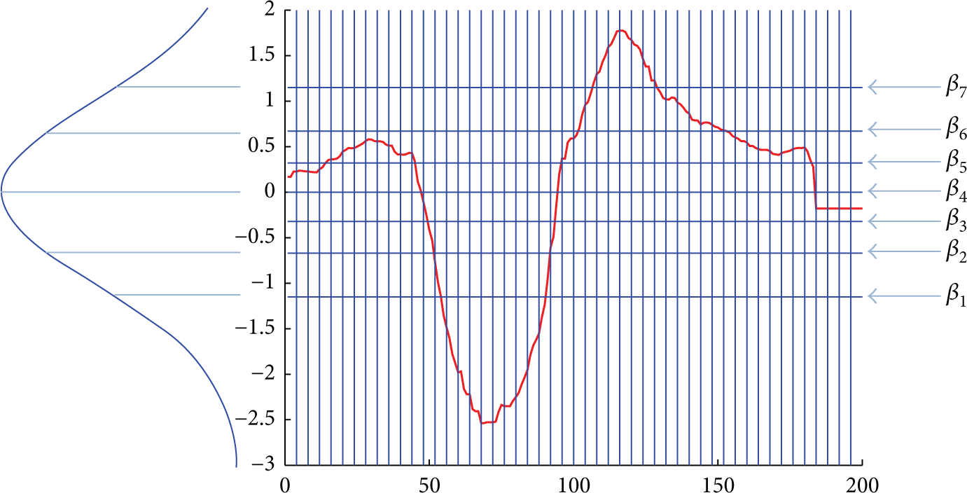
Mapping from original series to SAX symbolic representation: the vertical lines in graph divide the time series into pieces with equal length, and the horizontal lines divide the numerical range of different pieces into 8 sections according to Gaussian distribution.

Through this process, we are able to perform dimensional reduction and discretization. Meanwhile, as we need to compare the DTW distances, variation of the time series length may affect the results of the comparison. With the use of SAX, we can unify the length of the series obtained from different motion.

4.2. Feature Extraction Based on Distance Metric

The distance metrics that are commonly used in similarity estimation of time series include symbolic matching distances, different types of traditional distances, and DTW. Generalization of Euclidean distance in SAX representation provides us a lower bound distance based on the discrete symbolic data it generates. Assuming we have two symbolic series $s{t}_x\{x_{\mathrm{1}},x_{\mathrm{2}},\dots ,x_i,\dots ,x_{\text{low\_dim}}\}$ and $s{t}_y\{y_{\mathrm{1}},y_{\mathrm{2}},\dots ,y_j,\dots ,y_{\text{low\_dim}}\}$ , their lower bound distance can be calculated with (5). It is fast and effective in many application scenarios of time series mining, but it is only used in one-dimensional time series:

$$\begin{array}{cc}& \text{SAX\_MIN\_DIST}\left(s{t}_x,s{t}_y\right)=\sqrt{\frac{n_x+n_y}{\mathrm{2}\times \text{low\_dim}}}\sqrt{{\displaystyle \sum }_{i=\mathrm{1}}^{\text{low\_dim}}\text{min\_dist}{\left(x_i,y_i\right)}^{\mathrm{2}}}.\end{array}$$

(5)

$\mathrm{m}\mathrm{i}\mathrm{n}\_\mathrm{d}\mathrm{i}\mathrm{s}\mathrm{t}$ is calculated with

$$\begin{array}{cc}& \text{min\_dist}\left(x_i,y_i\right)=\left\{\begin{array}{cc}\mathrm{0},\hfill & \text{if}\left|x_i-y_i\right|\le \mathrm{1}\hfill \\ {\beta }_{\max \left(x_i,y_i\right)-\mathrm{1}}-{\beta }_{\max \left(x_i,y_i\right)},\hfill & \text{otherwise.}\hfill \end{array}\right.\end{array}$$

(6)

For multidimensional data, traditional distances such as Manhattan distance, Euclidean distance, and Mahalanobis distance are able to provide simple and fast similarity measurement. But these distances sequentially align two time series and cannot tolerate the offsets and time shifting. DTW is a proper way to solve these problems, but it costs too much time. Dynamic time warping is a pattern matching algorithm that can measure the similarity between two time sequences. It is first used in speech recognition and then spreads to other areas such as data mining, gesture recognition, and robotics. To speed up the calculation, we use Sakoe-Chiba band to restrict the matching range. 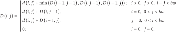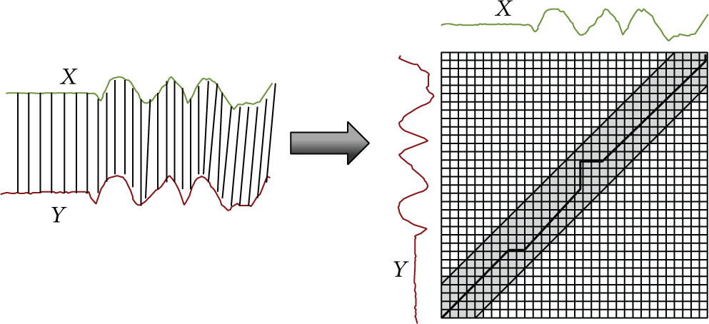For symbolic series $s{t}_x\{x_{\mathrm{1}},x_{\mathrm{2}},\dots ,x_i,\dots ,x_{\text{low\_dim}}\}$ and $s{t}_y\{y_{\mathrm{1}},y_{\mathrm{2}},\dots ,y_j,\dots ,y_{\text{low\_dim}}\}$ , this distance can be calculated using (7) as follows:

$$\begin{array}{cc}& D\left(i,j\right)=\left\{\begin{array}{cc}d\left(i,j\right)+\mathrm{m}\mathrm{i}\mathrm{n}\left(D\left(i-\mathrm{1},j-\mathrm{1}\right),D\left(i,j-\mathrm{1}\right),D\left(i-\mathrm{1},j\right)\right);\hfill & i>\mathrm{0},\hspace{0.17em}\hspace{0.17em}j>\mathrm{0},\hspace{0.17em}\hspace{0.17em}i-j<bw\hfill \\ d\left(i,j\right)+D\left(i,j-\mathrm{1}\right);\hfill & i=\mathrm{0},\hspace{0.17em}\hspace{0.17em}\mathrm{0}<j<bw\hfill \\ d\left(i,j\right)+D\left(i-\mathrm{1},j\right);\hfill & j=\mathrm{0},\hspace{0.17em}\hspace{0.17em}\mathrm{0}<i<bw\hfill \\ \mathrm{0};\hfill & i=\mathrm{0},\hspace{0.17em}\hspace{0.17em}j=\mathrm{0}.\hfill \end{array}\right.\end{array}$$

(7)

$bw\mathrm{\hspace{0.17em}\hspace{0.17em}}$ is the band width of the constraint. Normally, Euclidean distances are used to measure the similarity between data points $x_i$ and $y_j$ during the matching process as follows:

$$\begin{array}{cc}& d\left(i,j\right)=\sqrt{{\displaystyle \sum }_{k=\mathrm{1}}^{\dim }{\left(x_{ik}-y_{jk}\right)}^{\mathrm{2}}}.\end{array}$$

(8)

$\mathrm{d}\mathrm{i}\mathrm{m}$ is the dimension of each data point and $x_{ik}$ and $y_{jk}$ indicate data in kth dimension of $x_i$ and $y_j$ . The matching process is shown in Figure 4.

Figure 4

Demonstration of matching process of DTW: for two time series X and Y, their matching path is restricted in the diagonal belt area on the right, and the matching outside of this area will be ignored. This is a common way to speed up the calculation of this algorithm.

For dim-dimensional time series, we can either treat the data point at each time stamp as a dim-dimensional data and do the matching once or consider the matching on each dimension separately. These two methods may receive quite different results. Some studies [46] define the former one as $\mathrm{D}\mathrm{T}{\mathrm{W}}_D$ which would not allow different alignment on the same time stamp and the latter one as $\mathrm{D}\mathrm{T}{\mathrm{W}}_I$ that would accept the independent matching. The choice should be based on the correlation between different dimensions. In our case, we need to perform the matching on the symbolic series that does not support multidimensional situation. Therefore, we deal with the information from different DoF of various sensors independently. As a matter of fact, $\mathrm{D}\mathrm{T}{\mathrm{W}}_I$ is proved to be more effective than $\mathrm{D}\mathrm{T}{\mathrm{W}}_D$ in the existing studies of motion sensing. However, we do not sum up the distances on different DoFs as $\mathrm{D}\mathrm{T}{\mathrm{W}}_I$ . Instead, we consider each of them individually as one of the feature candidates. We will find out the most significant candidates with small correlation between each other in the next part.

4.3. Feature Selection Based on MCMR Strategy

As the selected series are treated as feature candidates, we decide to apply feature selection strategy in finding the most representative ones [47, 48]. In this section, Max-Correlation and Min-Redundancy (MCMR) strategy is proposed to screen out the features that best distinguish different classes and be independent from each other. It mainly consists of two steps: first of all, we find out the feature candidates with strong ability to distinguish samples from different classes; secondly, we need to eliminate the redundant candidates from the chosen ones. In the first step, we introduce the feature selection algorithm ReliefF to estimate the distinguished ability of each feature. By setting a certain threshold η for the number of candidates, we are able to filter out the features with strong correlations to the categories. In the next step, the candidates with weaker class correlation than their similar candidates are abandoned. Therefore, we need to sort the candidates obtained in the former step in descending order and then successively select the candidates with low correlation to the previous chosen ones until the termination condition is satisfied.

Definition 2 (RF weight: feature weight based on ReliefF).

RF weight is a value of a feature candidate that indicates its ability to distinguish different categories from each other. We can compute this weight with RelieF.

ReliefF [49] is a feature selection algorithm that can be applied in multiclass problem. It is the extended version of Relief which suits two-class problem only. In this algorithm, the weight of each feature will be determined after a few iterations. Specifically, in each iteration, ReliefF chooses one sample R from labelled data set randomly and then extracts k nearest neighbors (near hits) from the same category and k nearest samples (near misses) in every other category individually. After that, the weights of the features are updated based on the following:

$$\begin{array}{cc}& w\left(F_i\right)=w\left(F_i\right)-{\displaystyle \sum }_{j=\mathrm{1}}^k\frac{\mathrm{d}\mathrm{i}\mathrm{f}\mathrm{f}\left(F_i,R,H_j\right)}{mk}+{\displaystyle \sum }_{c\notin \mathrm{c}\mathrm{l}\mathrm{a}\mathrm{s}\mathrm{s}\left(R\right)}\frac{\left[\left(p\left(C\right)/\left(\mathrm{1}-p\left(\mathrm{c}\mathrm{l}\mathrm{a}\mathrm{s}\mathrm{s}\left(R\right)\right)\right)\right){\sum }_{j=\mathrm{1}}^k\mathrm{d}\mathrm{i}\mathrm{f}\mathrm{f}\left(F_i,R,M_j\left(C\right)\right)\right]}{mk}.\end{array}$$

(9)

The $\mathrm{d}\mathrm{i}\mathrm{f}\mathrm{f}$ function is defined in

$$\begin{array}{cc}& \mathrm{d}\mathrm{i}\mathrm{f}\mathrm{f}\left(F_i,R_{\mathrm{1}},R_{\mathrm{2}}\right)=\left\{\begin{array}{cc}\frac{\left|R_{\mathrm{1}}\left(F_i\right)-R_{\mathrm{2}}\left(F_i\right)\right|}{\mathrm{m}\mathrm{a}\mathrm{x}\left(F_i\right)-\mathrm{m}\mathrm{i}\mathrm{n}\left(F_i\right)},\hfill & \text{if}\hspace{0.17em}\hspace{0.17em}{F}_i\text{\hspace{0.17em}\hspace{0.17em}is\hspace{0.17em}\hspace{0.17em}continuous}\hfill \\ \mathrm{0},\hfill & \mathrm{i}\mathrm{f}\hspace{0.17em}\hspace{0.17em}F\mathrm{i}\mathrm{s}\mathrm{d}\mathrm{i}\mathrm{s}\mathrm{c}\mathrm{r}\mathrm{e}\mathrm{t}\mathrm{e}\mathrm{a}\mathrm{n}\mathrm{d}{R}_1\left(F_i\right)=R_{\mathrm{2}}\left(F_i\right)\hfill \\ \mathrm{1},\hfill & \mathrm{i}\mathrm{f}F\mathrm{i}\mathrm{s}\mathrm{d}\mathrm{i}\mathrm{s}\mathrm{c}\mathrm{r}\mathrm{e}\mathrm{t}\mathrm{e}\mathrm{a}\mathrm{n}\mathrm{d}{R}_{\mathrm{1}}\left(F_i\right)\ne R_{\mathrm{2}}\left(F_i\right).\hfill \end{array}\right.\end{array}$$

(10)

F is a collection of feature candidates chosen from labelled data of different classes. $w(F_i)$ is the RF weight of the ith feature candidate; $H_j$ is the jth nearest hits; $M_j(C)$ is the jth nearest misses in class C. $\max \hspace{0.17em}(F_i)$ and $\min \hspace{0.17em}(F_i)$ represent the maximum and minimum values of $F_i$ .

After a certain time of iterative computations, features that can better distinguish samples from different classes will obtain higher weights. However, in the process above, feature candidates are supposed to be independent from each other, and they do not consider the correlation and redundancy between features. Therefore, we need to eliminate the redundant candidates. Here, we first sort the features in descending order based on their RF weights and remove the candidates with weights less than a certain threshold. Then, for the rest of the candidates, we should check whether they are correlated with the chosen ones, successively. If one candidate is supposed to have close relationship with one of the chosen features, it should be abandoned. Otherwise, it can be kept as one of the chosen features. This process will continue until we have collected enough number of features.

In previous studies, various measurements are used to estimate feature redundancy, such as information gain, mutual information, and correlation coefficient. We notice that redundant candidates usually have similar class separability, which means their RF weights have higher linear correlation with each other. Here we use Pearson correlation coefficients based on the RF weights to indicate the correlation between the candidates, which is indicated in the following:

$$\begin{array}{cc}& {\rho }_{a,b}=\frac{\sum w_a{w}_b-\sum w_a\sum w_b/N}{\sqrt{\left(\sum w_a^{\mathrm{2}}-{\left(\sum w_a\right)}^{\mathrm{2}}/N\right)\left(\sum w_b^{\mathrm{2}}-{\left(\sum w_b\right)}^{\mathrm{2}}/N\right)}}.\end{array}$$

(11)

We use $w_a$ to represent the RF weight matrix of a chosen feature and $w_b$ indicates the RF weight matrix of a candidate. ${\rho }_{a,b}$ is the Pearson correlation coefficient between a feature that has already been chosen and a candidate. If this correlation coefficient is higher than the threshold, then we should eliminate this candidate.

Pearson correlation coefficient estimates the linear correlation between two variables. Its value is between +1 and −1 inclusive, where 1 is total positive correlation, 0 means no correlation, and −1 is total negative correlation. The actual correlation situation is described in Table 2. According to these corresponding relations, the threshold is easy to define. And this is why we choose this method.

Table 2

Correlation situation represented by Pearson correlation coefficients.

Correlation coefficients range	Correlation situation
1.0∼0.8	Extremely strong relation
0.8∼0.6	Strong relation
0.6∼0.4	Medium correlation
0.4∼0.2	Weak correlation
0.2∼0.0	Extremely Weak correlation/no relation
0.0∼−1.0	Negative correlation

The pseudocode of this process is shown in Algorithm 1.

Algorithm 1: MCMR_FeatureSelection(Dis, sn, k, cft, $\mathrm{\eta }$ ).

Input:

   $\mathrm{D}\mathrm{i}\mathrm{s}$ as distance vector

   $\mathrm{s}\mathrm{n}$ as sampling times in ReliefF

  k as numbers of nearest hits and misses in ReliefF

  $\hspace{0.17em}\mathrm{c}\mathrm{f}\mathrm{t}$ as cut off threshold of max class correlation candidates

   $\mathrm{\eta }$ as the threshold of correlation coefficient;

Output:

   $best\hspace{0.17em}\hspace{0.17em}f$ as a group of Max-Correlation and Min-Redundancy features

(1)  W $\leftarrow$ ReliefF( $\mathrm{D}\mathrm{i}\mathrm{s}$ , $\mathrm{s}\mathrm{n}$ , k); {calculate the RF weight: W}

(2)   $\mathrm{s}\mathrm{i}\mathrm{d}$ $\leftarrow$ sort(W); {find the descending order of W}

(3)  i $\leftarrow$ cutoff( $\mathrm{s}\mathrm{w}$ , $\mathrm{c}\mathrm{f}\mathrm{t}$ ); {find the turing position of cft}

(4)   $best\hspace{0.17em}\hspace{0.17em}f\leftarrow \mathrm{⌀}$ ;

(5)   $best$ .add( $\mathrm{s}\mathrm{i}\mathrm{d}$ (1));

(6)   $j\leftarrow \mathrm{2}$ ;

(7)   $\mathrm{n}\mathrm{u}\mathrm{m}\leftarrow \mathrm{1}$ ;

(8)  while   $j<i$   do

(9)    $k\leftarrow \mathrm{1}$ ;

(10)  while   $k<best\hspace{0.17em}f$ .size( )  do

(11)   if   ${\mathrm{\rho }}_{\mathrm{s}\mathrm{i}\mathrm{d}(j),best\hspace{0.17em}f(k)}>\mathrm{\eta }$   then

(12)    break;

(13)   else

(14)     $k\leftarrow k+\mathrm{1}$ ;

(15)   end if

(16)  end while

(17)  if   $k==\mathrm{n}\mathrm{u}\mathrm{m}+\mathrm{1}$   then

(18)    $\mathrm{n}\mathrm{u}\mathrm{m}=\mathrm{n}\mathrm{u}\mathrm{m}+\mathrm{1}$ ;

(19)    $best\hspace{0.17em}f$ .add( $\mathrm{s}\mathrm{i}\mathrm{d}(j)$ );

(20)  end if

(21)   $j=j+\mathrm{1}$ ;

(22) end while

With this procedure, we are able to screen out features with high class correlation and low redundancy. These features can be used to build various kinds of classifiers for motion recognition.

4.4. Motion Classification

In this stage, we can use the selected features to train different kinds of classifiers, such as 1-Nearest Neighbor [50], Bayes Net [51], and Random Forest [52]. We may obtain different results from various classifiers, and we should choose the proper one with better performance in actual application after a few trials. In our study, we apply this solution in dance action practice. The classification effect will be discussed in detail in the next section.

5. Experiments

To verify the efficiency of our solution, we discuss its application in dance practice. The motion data is collected with smart phone and recognize different movements and gestures performed by the wearers. In fact, we found large amount of such requirements as detecting human movements during the practice session in physical education. In our case, we invite 5 students to perform 6 basic practice movements. Each movement is performed 10 times by each person. We perform 10-fold cross-validation on these data to check the classification results in MATLAB.

In this section, we are going to discuss the following problems:

• (i)

Feasibility and superiority of the solution.

(ii)

Necessity of sensor fusion.

(iii)

Parameters selection and adjustment.

More details can be found in the rest of this section.

5.1. Feasibility and Superiority Verification

In order to check the feasibility and superiority of our solution in multivariant motion series recognition, we compare its classification accuracy with the commonly used methods. For multidimensional time series, there are actually two ways to measure the distance based on DTW. We can either calculate the matching cost on each dimension separately or match the multidimensional data points all together in one time. According to [46], this decision should be based on the correlation between these dimensions. As a matter of fact, these two methods have both been applied in related studies. In our solution, we consider the dimensions independently and leave the correlation problem to feature selection process. To check the superiority of our solution, we also try the other ways, including using LB instead of DTW, three kinds of DTW matching without symbolization. In this comparison, we set lower dimension as 50, k as 5, and η as 0.5. The accuracies in different classifiers are shown in Figure 5.

Figure 5

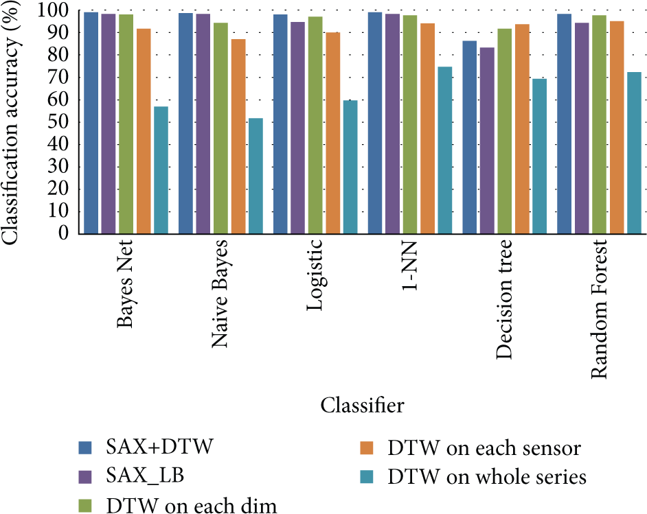
Classification accuracies in various classifiers with different solution: our solution uses DTW on time series represented by SAX and obtains the best and stable results with different classifiers most of the time. SAX_LB also performs quite good with its high efficiency. DTW on original time series does not reveal outstanding performance with exact matching. Specifically, $\mathrm{D}\mathrm{T}{\mathrm{W}}_I$ performs better than $\mathrm{D}\mathrm{T}{\mathrm{W}}_D$ .

At the same time, we should also take a look at the time cost of each solution in training and testing in Figure 6.

Figure 6

Time consumption of different solutions: SAX_LB is the fastest with no doubt as it only performs synchronous matching. $\mathrm{D}\mathrm{T}\mathrm{W}$ takes much time as expected, especially for $\mathrm{D}\mathrm{T}{\mathrm{W}}_I$ . By aligning with symbolic series, we speed up our solution and get the second place among these similarity measurements.

As we can see from the results above, measuring DTW distance on different dimensions separately performs better than multidimensional comparison. If we consider the dimensional fusion on each sensor, it will take too much time with ordinary performance. If we take the whole series together with all dimensions to calculate the distance, the result will be disappointing, though it does not take much time.

It is quite obvious that the symbolic representation would not reduce the classification accuracy while reducing calculation time. In contrast, symbolic representation performs a little bit better than original series using DTW, most of the time. To overcome the time shifting and offsets of the motion data, we apply DTW on the symbolic series. As we expected, this solution obtains the best classification accuracy and takes less time than DTW comparison on the original data. As a matter of fact, lower bound distance of SAX takes the least time in training and testing. And its accuracy is acceptable. Thus, it is also a good trade-off between time and accuracy.

5.2. Discussion of Sensor Fusion

Most of the existing studies would use a single accelerometer to measure the motion state, while some may also consider the readings of gyroscope or magnetometer. Here in our situation, we are able to obtain information from various sensors. How to choose proper amount of data to achieve better performance has become one of our research goal. In one hand, we check the performances with the use of only one kind of sensor data in Figure 7.

Figure 7

Classification accuracies using data of each sensor separately: it is quite obvious that if we use different types of sensor information independently, accelerometer and its transformation win in most of the time. However, the results do not seem to be improved after the transformation into Earth coordinates.

From these results, we confirm that accelerometer is the most effective sensor among the existing sensing groups. Most sensors behave better using 1-NN, and a little worse with decision tree. If we observe the results independently, we discover that the original reading from accelerometer containing the influence of gravity performs a little better than pure linear acceleration alone. For gyroscope, the results are improved after the preprocessing such as eliminating the bias. The transformation into Euler angles obtains better performance, but the quaternion does not work so well alone. Gravity and magnetometer obtain mediocre results separately. Meanwhile the transformation into Earth coordinates does not seem to improve much. Among all these results, the best performance comes from the linear acceleration in Earth coordinates, which obtains 97% classification accuracy using 1-NN.

On the other hand, we are going to find out the situation in sensor fusion. Whether it is necessary to use data from different sensors in our situation is one question we need to answer. Therefore, we discuss the performance using the fusion data in Figure 8.

Figure 8

Classification accuracies with sensor fusion: we get better results with more information. In fact, there are slight differences between different kinds of fusion. And it is unnecessary to use all the data in actual practice.

Obviously, the results of sensor fusion are much higher than single sensing data. From the overall performance viewpoint, fusion of all sensor data behaves the best, when fusion of CMDeviceMotion (CMDM) data performs better than fusion of four key sensors: accelerometer, gyroscope, gravity sensor, and magnetometer $(\mathrm{A}\mathrm{c}+\mathrm{G}\mathrm{y}+\mathrm{G}\mathrm{r}+\mathrm{M}\mathrm{a})$ in CMDeviceMotion. And the performance of four key sensors in CMDeviceMotion is better than fusion of their raw data in most of the time. The results of accelerometer and gyroscope fusion are relatively worse than the other fusions. Among all these results, we have the best performance coming from fusion of all with 99.33% classification accuracy using 1-NN.

Apparently, with our solution, sensor fusion improves the performance. With more types of sensor data, we would have more information from different points of view. But, at the meantime, we should also consider the time consumption. Our final choice should be based on the resources we have, and the trade-off between time and accuracy might be the best decision.

5.3. Parameter Setting

To obtain better performance, we need to choose proper parameters. And one of the common ways to achieve this goal is to decide through experiments. In our solution, we will discuss three important factors. Firstly, we should mind the choice of target dimension of discrete segmentation. If this size is too small, it will affect the accuracy. If it is too large, it will take too much time. Here, we compare the accuracy in different classifiers with different size of the target dimensions in Figure 9. And the average of the accuracies of different classifiers is shown in Figure 10, which indicates the overall trend of performance with different size of the target dimensions.

Figure 9

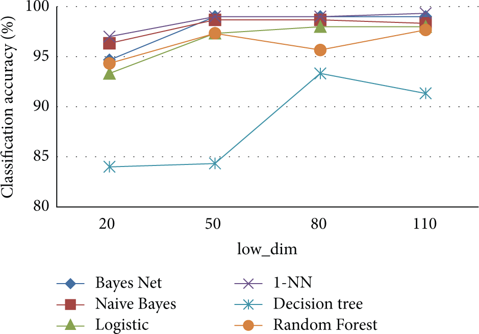
Classification accuracies of different classifiers with different size of the target dimensions: most of the classifiers achieve high accuracies above 90%. With the growth of low_dim in symbolic representation, we have longer series and obtain better results. Thus the trend of classification accuracies generally goes up.

Figure 10

Average classification accuracies with different size of the target dimension: the overall trend of classification accuracies grows as the increase of the length of the symbolic representation and becomes steady after 80. As the compression ratios are lower with high target dimensions, the new series reserve more information for classification.

Meanwhile, we should also take a look at the time cost of these situations. And the results are shown in Figure 11.

Figure 11

Time consumption with different size of the target dimension: there is a clear growth of time consumption along with the increase of low_dim, as with longer series we need more matching and calculation.

From these results, we can see that for most classifiers, 50 would be a better choice as it takes less time while obtaining fairly well accuracy. Secondly, the threshold of Pearson correlation coefficient η is another parameter we need to observe. According to our intuition, candidates with high correlations to the chosen features might be redundant and should be eliminated. Thus, we should find a threshold to filter out those candidates. As we have mentioned above, this correlation coefficient is defined in a small range, and we can find out the correlation situation based on the interval this value falls in. Now, let us see where we should put this threshold. Since the range of this value is quite narrow, we can easily cover the whole positive range. The performance in different situations is shown in Figures 12 and 13.

Figure 12

Classification accuracies with different η: this is a discussion of the correlations between chosen features. If η is too small, the results of most classifiers are lower, as many useful features are abandoned. Meanwhile, if it is too big, we would reserve too many features, including the redundant ones, which may also affect the result.

Figure 13

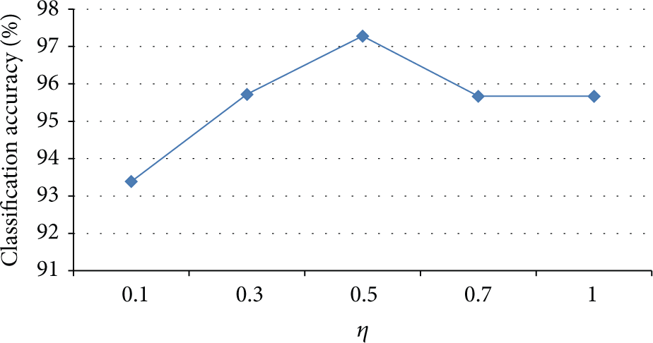
Average accuracies of different classifiers with different η: the overall trend of the accuracies on different classifiers goes up until it pass 0.5 and drops a little afterwards. This result accords with the nature of relationship between the number of features and the classification results.

According to this result, we learn that medium correlations around 0.5 work for our case. This fact actually accords with logic and our expectation. Finally, we take a look at the choice of k in RF weight calculation, which represents the number of nearest candidates we need to consider in different classes. It is commonly believed that the nearest few samples play a significant role in estimating class discrimination ability as they are easier to be confused. So, we check the performance with different choices of k, and the results are shown in Figures 14 and 15.

Figure 14

Classification accuracies of different classifiers with different k: no matter what kind of classifiers we use, the results do not change much with different number of nearest samples chosen from various categories for feature estimation.

Figure 15

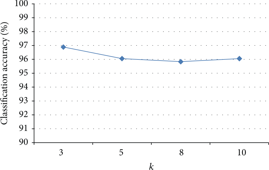
Average accuracies of different classifiers with different k: it does not show significant changes in performance with only slight decrease in average accuracies, using different number of nearest samples to estimate the quality of the feature candidates.

As we can see from the results, no significant change appears in situations with different k, only a slight decline in the trend of average accuracy. That means the performance is insensitive to k in this range. It takes less energy in setting this parameter.

6. Conclusion and Future Work

In this paper, we propose a flexible and efficient solution for motion recognition. This solution measures the human movements and gestures using smart phone embedded sensors and applies Max-Correlation and Min-Redundancy strategy to select proper features based on interclass symbolic distance metric. In order to decide what kinds of sensors are needed, we test the effect of different sensors individually as well as combinations of various sensors. The final choice should be a trade-off between time and accuracy based on the requirement and resources. If we pay more attention to efficiency, we can choose less sensor data with accuracy around 94% in average, whereas we can obtain about 98% accuracy using more sensor information. In general, fusion of a few key sensors would be a better option in most cases. In our situation, we believe fusion of accelerometer and gyroscope with 6 dimensions reaching accuracies around 95.67% in average and 98.33% at best would be a better trade-off between time and accuracy. In data recognition phase, the symbolic representation is able to reduce the dimension of the time series that speeds up the calculation while eliminating the noise and random disturbances. Dynamic time warping on this low dimensional discrete data overcomes the influences of data offsets and time shifting and, in the meantime, improves the classification accuracy. To find out the significant distance measurements and use them as classification features, we define RF weights based on ReliefF algorithm to estimate their class correlation and remove the redundant ones based on Pearson correlation coefficient. This solution is proved to be quite effective in real world application of motion detection in dance practice. In fact, the methods we used in the structure of our solution can be replaced with other related methods based on actual needs, which is quite flexible.

This study is mainly a preliminary exploration of the feasibility of the method. Our future job is to serve more applications by training our solution for more types of movements in dance classes as well as other disciplines such as martial art and gymnastics.