Energy-Efficient Data Recovery via Greedy Algorithm for Wireless Sensor Networks

Abstract

Accelerating energy consumption and increasing data traffic have become prominent in large-scale wireless sensor networks (WSNs). Compressive sensing (CS) can recover data through the collection of a small number of samples with energy efficiency. General CS theory has several limitations when applied to WSNs because of the high complexity of its ${\mathcal{l}}_1$ -based conventional convex optimization algorithm and the large storage space required by its Gaussian random observation matrix. Thus, we propose a novel solution that allows the use of CS for compressive sampling and online recovery of large data sets in actual WSN scenarios. The ${\mathcal{l}}_0$ -based greedy algorithm for data recovery in WSNs is adopted and combined with a newly designed measurement matrix that is based on LEACH clustering algorithm integrated into a new framework called data acquisition framework of compressive sampling and online recovery (DAF_CSOR). Furthermore, we study three different greedy algorithms under DAF_CSOR. Results of evaluation experiments show that the proposed sparsity-adaptive DAF_CSOR is relatively optimal in terms of recovery accuracy. In terms of overall energy consumption and network lifetime, DAF_CSOR exhibits a certain advantage over conventional methods.

1. Introduction

A wireless sensor network (WSN) is a system that involves information collection, transmission, and processing. It is widely utilized in environmental monitoring, military defense, health monitoring, smart homes, and many other important fields. WSNs have attracted an increasing amount of attention from the academia because of their extensive application. As the scale of WSNs continues to expand, energy consumption and transmission costs increase as well. There are some methods to decrease the energy consumption and transmission costs. One way is to increase the number of sinks during the deployment. Another alternative way is to design the compressed algorithm during the transmission. We apply compressive sensing (CS) to WSNs in this study to address this problem. CS technology [1, 2] employs a much lower sampling rate than the frequency present in the original signal to sample signals; it is far more effective than the Nyquist sampling theorem [3]. Compressive sampling can reduce the amount of data sent, received, and processed by WSN nodes to save energy.

Over the past few years, many scholars have studied the application of CS in WSNs. The authors in [4] employed principal component analysis (PCA) [5] to capture the spatial and temporal characteristics of real signals and analyze the combined use of CS and PCA with a Bayesian framework. Reference [6] investigated the adoption of CS in WSNs by considering network topology and routing, which is utilized to transport random projections of the sensed data to the sink. However, the performance was not as good as expected [6]. Conventional ${\mathcal{l}}_1$ minimization is unsuitable for large-scale WSN signal recovery because of its high algorithm complexity; in addition, it usually adopts Gaussian random observation, which requires a large transmission cost [4]. Thus, applying conventional CS theory to WSNs natively cannot result in good recovery performance and high energy efficiency. Reference [7] employed the LEACH algorithm [8, 9] to perform node clustering and recover the source through Bayesian CS. Reference [10] utilized the LEACH algorithm to improve the random sampling process.

In this study, we focus on how to approximately perform signal recovery with high accuracy (over 90%) and reduce the energy consumption at the same time. Considering that the greedy algorithm, which is a heuristic algorithm that uses the locally optimal choice at each stage rather than a global optimum, has the advantages of low computational complexity and high computational speed [11], we apply this algorithm to WSNs to approximate data recovery. Moreover, we utilize the spatial correlation among WSN nodes in combination with LEACH method to design a measurement matrix and conduct compressed sampling and approximate reconstruction in an energy-efficient manner. Lastly, we design and implement a new framework called data acquisition framework of compressive sampling and online recovery (DAF_CSOR). We conduct a detailed analysis and comparison of three different algorithms under DAF_CSOR in actual WSN scenarios and conclude that DAF_CSOR is relatively optimal. The main contributions of this study are as follows:

• (i)

In view of the real signal in WSNs, we design DAF_CSOR and construct the observation matrix through LEACH clustering.

(ii)

We study three different recovery methods based on the greedy algorithm to optimize DAF_CSOR.

(iii)

We conducted a detailed analysis and performed a comparison of three different algorithms under the DAF_CSOR framework in real WSN scenarios. We selected DAF_CSOR_SAMP as a signal recovery algorithm due to its sparsity-adaptive capability. It not only has high recovery accuracy but also guarantees extended WSN lifetime.

This paper is structured as follows. The traditional CS framework of sensing, compression, and recovery is presented in Section 2. DAF_CSOR for compressive sampling and online recovery is proposed in Section 3, and three different recovery methods are investigated based on the greedy algorithm. The distributed signal model and simulation results are presented in Section 4. Here, we confirm that the assumptions under DAF_CSOR are effective for real-world signals. The conclusions of the study are presented in Section 5.

2. CS Basics

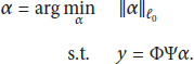
In conventional CS theory, the natural physical signal is represented as vector $x\in R^N$ , where N is the vector length. Specifically, an invertible transformation matrix Ψ of size $N\times N$ must exist, such that

$$\begin{array}{c}x=\Psi \alpha ,\\ {‖\alpha ‖}_{l_0}=k,\hspace{1em}k\ll N,\end{array}$$

(1)

where $\alpha \in R^N$ . If α has k nonzero elements, then α is a k-sparse representation of x. We applied commonly used discrete cosine transform (DCT) to the sparse signal.

Through random sampling of the sparse transform coefficients of the original signal, we write

$$\begin{array}{c}y=\Phi x=\Phi \Psi \alpha ,\end{array}$$

(2)

where $y\in R^M$ refers to linear observations obtained through random sampling and $\Phi \in R^{M\times N}$ represents measurement matrix $M\ll N$ .

Measurement matrix $\Phi \in R^{M\times N}$ is fixed and does not depend on the signal itself. To reconstruct the sparse or compressible signal, the measurement matrix should meet the restricted isometry property (RIP) [12]; that is, for any k-sparse vector x, $0<{\delta }_k<1$ exists to establish

$$\begin{array}{c}\left(1-{\delta }_k\right){‖x‖}_2\le {‖\Phi x‖}_2\le \left(1+{\delta }_k\right){‖x‖}_2.\end{array}$$

(3)

Then, Φ is said to satisfy RIP.

Commonly utilized measurement matrices include Gaussian white noise matrix [13], ±1 Bernoulli matrix, and sub-Gaussian random measurement matrix. The common characteristic of these measurement matrices is that the matrix elements independently obey a certain distribution. Such measurement matrices are incoherent with most sparse signals; thus, precise reconstruction requires a small number of observations. However, these matrices do not have the characteristics of distributed networks and often require large storage space and high computational complexity. Therefore, adopting this type of measurement matrix in data compression is unsuitable for WSNs. Consequently, we designed the Gaussian random measurement matrix based on clustering.

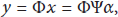
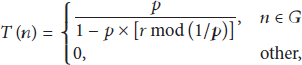
Finally, the estimation of sparse coefficient α is recovered via sample vector y and the measurement matrix. This problem must be solved with a recovery algorithm that can be described as

$$\begin{array}{c}\alpha =\mathrm{a}\mathrm{r}\mathrm{g}\hspace{0.17em}\underset{\alpha }{\mathrm{m}\mathrm{i}\mathrm{n}}\hspace{1em}{‖\alpha ‖}_{{\mathcal{l}}_0}\\ \mathrm{s}.\mathrm{t}.\hspace{1em}y=\Phi \Psi \alpha .\end{array}$$

(4)

According to (4), ${\mathcal{l}}_0$ minimization is generally an NP-hard problem that cannot be effectively solved at present. Two types of methods, namely, ${\mathcal{l}}_0$ -based greedy algorithm and ${\mathcal{l}}_1$ -based convex optimization problem, are employed for this problem. ${\mathcal{l}}_1$ -based convex optimization problem is unsuitable for large-scale WSNs because of its high algorithm complexity. Therefore, we focused on ${\mathcal{l}}_0$ -based greedy algorithm.

3. DAF_CSOR and Recovery Method Based on the Greedy Algorithm

DAF_CSOR is presented in this section. The structure of the measurement matrix based on LEACH algorithm is investigated, and the coherence of the measurement matrix is analyzed. Finally, we focus on three different recovery methods based on the greedy algorithm (CoSaMP, ROMP, and SAMP) to optimize DAF_CSOR.

3.1. DAF_CSOR

As shown in Figure 1, DAF_CSOR includes three parts, namely, sensing, compression, and online recovery. We performed sensing and compression of the original physical signals by using measurement matrix Φ and sparse matrix Ψ. We selected DCT as a sparse matrix, utilized LEACH algorithm for node clustering in WSNs, and constructed the measurement matrix based on the clustering (Section 3.2). Online recovery is the focus of our study, and three recovery methods, namely, DAF_CSOR_CoSaMP, DAF_CSOR_ROMP, and DAF_CSOR_SAMP, were investigated based on the greedy algorithm (Section 3.3). We investigated each of the components of the framework.

Figure 1

DAF_CSOR.

3.2. Design of the Measurement Matrix

The CS technique and the LEACH method are both well known techniques. However, they cannot be used well if we combine them in their native forms [6]. To use the CS technique and construct an appropriate measurement matrix, we modified the LEACH method. Unlike the original LEACH method, where there was no need to consider the number, randomness, and coherence of the cluster head selection, we select the cluster heads based on the following three points.

$(1)$ The number of cluster heads should be at least $4\times k$ (where k is a sparsity coefficient).

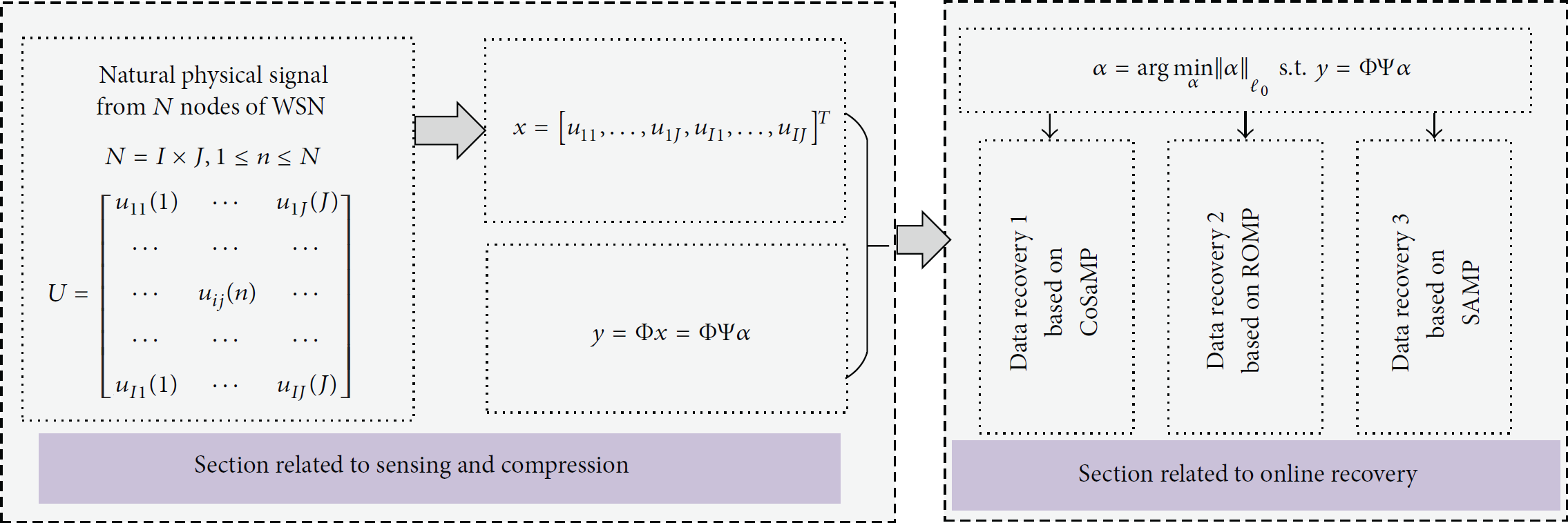
During the cluster election phase, the selection of each node as a cluster head or not depends on the percentage of cluster heads in WSNs and the number of times of it being a cluster head. If the node's remaining energy is smaller than the threshold, then the node no longer qualifies as a cluster head. Unlike the general LEACH algorithm, the number of cluster heads depends on the number of rows of observation vector based on the combination of CS theory, which should be at least $4\times k$ (k is a sparse coefficient).

$(2)$ The decision on whether or not the current node becomes the cluster head of the current round is made based on formula (5).

Each node generates a random number ranging from 0 to 1. If the number is smaller than the threshold $T(n)$ and the current node has not become a cluster head yet, then it becomes the cluster head of the current round. The threshold formula is as follows:

$$\begin{array}{c}T\left(n\right)=\left\{\begin{array}{cc}\frac{p}{1-p\times \left[r\hspace{0.17em}\mathrm{m}\mathrm{o}\mathrm{d}\left(1/p\right)\right]},\hfill & n\in G\hfill \\ 0,\hfill & \text{other,}\hfill \end{array}\right.\end{array}$$

(5)

where p is the percentage of nodes becoming cluster heads, r is the current round number, and G is the set of nodes that have not become cluster heads in recent $1/p$ rounds. During the cluster setup phase, after each node opts to join the nearest cluster head, the nodes within a cluster send their data to the cluster head and update their own energy. The sink node extracts the observation vector from all the cluster heads and sets the value of the local head node to “1” and that of the other nodes in this cluster to “0.” Cluster number is the number of “1” in the observation matrix.

$(3)$ The coherence between the measurement matrix and the sparse transformation matrix must be calculated using formula (6). Lower coherence leads to higher recovery here.

Finally, a measurement matrix of size $4k\times N$ is built. The coherence of the measurement matrix after the construction of the observation matrix must be analyzed to stably recover the compressed data. Coherence is calculated as

$$\begin{array}{c}\text{Coherence}\hspace{0.17em}\mu =\underset{i\ne j}{\mathrm{m}\mathrm{a}\mathrm{x}}〈H_i,H_j〉.\end{array}$$

(6)

The correlation between measurement matrix Φ and sparse transformation matrix Ψ depends on the column of matrix $\Phi \Psi$ . $H_i=\Phi {\psi }_i,H_j=\Phi {\psi }_j$ , so the inner product of $H_i$ and $H_j$ can be described as $〈H_i,H_j〉={{\psi }_i}^T{\Phi }^T\Phi {\psi }_j$ .

The probability of “0” or “1” appearing in each row of the Gaussian random measurement matrix is fixed; thus, the coherence calculations of the Gaussian random measurement matrix generated in each experiment show minimal change. As the number of cluster heads M increases, the number of “1” in the measurement matrix also increases. The coherence formula indicates that the correlation decreases while the corresponding recovery stability increases. DAF_CSOR focuses on stable recovery with low coherence.

3.3. Energy-Efficient Data Recovery via the Greedy Algorithm

Energy-efficient data recovery is a key step of the application of CS in WSNs. On the one hand, according to the Section 3.2, there is a subset of sensor nodes that participate in the CS process, so that the method can cut the number of transmitted data and reduce the overall energy cost. On the other hand, it is true that energy consumption must exist for the data recovery of CS. However, taking inspiration from references [4, 14], we let the data recovery process by using greedy algorithm occur at the sink node; that is, we only perform the computation required for compressive sensing at the sink node, where there are no stringent energy requirements. The ${\mathcal{l}}_0$ -based greedy algorithm can be described as follows:

$$\begin{array}{c}\underset{x}{\mathrm{m}\mathrm{i}\mathrm{n}}\hspace{1em}{‖x‖}_0\\ \mathrm{s}.\mathrm{t}.\hspace{1em}y=\Phi \Psi \alpha .\end{array}$$

(7)

After obtaining the estimated value of sparse coefficient α, we performed inverse transformation of α, that is, $x=\Psi \alpha$ , to obtain the recovered signal. In this section, three types of energy-efficient recovery methods based on the greedy algorithm under DAF_CSOR are described in detail.

3.3.1. DAF_CSOR_CoSaMP

The algorithm utilized in DAF_CSOR_CoSaMP method is derived from RIP. Assuming that ${\delta }_k\ll 1$ is the RIP parameter in the measurement matrix, for k-sparse signal x, the energy of the subsets formed by every k component is approximately equal to that of the corresponding k components of signal x. Thus, vector $c={\Phi }^T\Phi x$ can be utilized as a signal proxy. Given that $y=\Phi x$ , we only need to compute ${\Phi }^T\Phi x$ to obtain the equivalent representation of target signal x. The residual was included in the updated estimates at each iteration, and the position of the largest component from the residual was determined. Next, the target signal with these samples was estimated via least squares method. This process was repeated until ${‖r_k-r_{k-1}‖}_2<\delta$ , where δ is the threshold of residual error. The specific steps are shown in Algorithm 1.

Algorithm 1: DAF_CSOR_CoSaMP method.

Input: Measurement matrix $\mathrm{\Phi }\in R^{M\times N}$ , noisy sample vector $y\in R^M$ , sparsity level k

Output: k-sparse approximation $\widehat{x}$ of target signal

Initialization: Initial approximation $x_0=0$ , residual $r_0=y$ , and iteration $t=1$

repeat

 ( $\mathit{1}$ ) Signal proxy: $c={\mathrm{\Phi }}^T{r}_{t-1}$

 ( $\mathit{2}$ ) Identify large components and merge supports: $\mathrm{\Omega }=\sup \left(c_{2k}\right)$ , $T=\mathrm{\Omega }\cup \sup \left(x_{t-1}\right)$

 ( $\mathit{3}$ ) Signal estimation by least squares:

   $b{\left|\right.}_T={\mathrm{\Phi }}_T^{+}y$ , $b{\left.\right|}_{T^c}=0$

 ( $\mathit{4}$ ) Prune to obtain next approximation: $x_t=b_k$

 ( $\mathit{5}$ ) Update current residual: $r_t=y-\mathrm{\Phi }{x}_t$

until halting criterion is met

3.3.2. DAF_CSOR_ROMP

This method calculates correlation coefficient $u=\left\{u_j\mid u_j=\left|〈r,{\varphi }_j〉\right|,j=\mathrm{1,2},\dots ,N\right\}$ by computing the absolute value of the inner product between each atom (column vector) in matrix Φ and residual r while adding the selected atom that has the largest correlation coefficient calculated for each time to candidate set J. This process is regarded as the first atomic screening. After the formation of the candidate set, we introduced the regularization ideas for the second screening of candidate set J. The atoms in the collection are divided into several groups according to the correlation coefficient $\left|u(i)\right|\le 2\left|u(j)\right|$ , $i,j\in J$ . After grouping, we selected a set of measurement matrix column vectors (atoms) whose correlation coefficient has the largest energy. We then stored the corresponding indexes to ${\Lambda }_0$ . This process of atom selection can ensure that support set ${\Phi }_{\Lambda }$ can be obtained after at most k iterations. For those atoms that were not elected, the process of regularization ensures that their energy is less than that of the elected ones. After obtaining a support set for the reconstruction of the signal, we updated the residual and performed signal approximation by least squares method. The specific steps are shown in Algorithm 2.

Algorithm 2: DAF_CSOR_ROMP method.

Input: Measurement matrix $\mathrm{\Phi }\in R^{M\times N}$ , noisy sample vector $y\in R^M$ , sparsity level k

Output: k-sparse approximation $\widehat{x}$ of target signal

Initialization: $r_0=y$ , $\mathrm{\Lambda }=\mathrm{⌀}$ , ${\mathrm{\Lambda }}_0=\mathrm{⌀}$ , $J=\mathrm{⌀}$ and iteration $t=1$

repeat

 ( $\mathit{1}$ ) Correlation coefficient: $u_t={\mathrm{\Phi }}^T{r}_{t-1}$

 ( $\mathit{2}$ ) Find k maximum values from $u_t$ and store the corresponding indexes into J

 ( $\mathit{3}$ ) Regularize the correlation coefficient of the atoms corresponding to the indexes of J,

   select index values satisfying $\left|u_i\right|\le 2\left|u_j\right|$ in ${\mathrm{\Lambda }}_0$

 ( $\mathit{4}$ ) Update support set ${\mathrm{\Phi }}_{\mathrm{\Lambda }}:\mathrm{\Lambda }=\mathrm{\Lambda }\cup {\mathrm{\Lambda }}_0$

 ( $\mathit{5}$ ) Signal approximation:

   $\widehat{x}=\arg \mathrm{m}\mathrm{i}\mathrm{n}{‖y-{\mathrm{\Phi }}_{\mathrm{\Lambda }}{x}_{t-1}‖}_2$

 ( $\mathit{6}$ ) Update current residual: $r=y-{\mathrm{\Phi }}_{\mathrm{\Lambda }}\widehat{x}$

until halting criterion is met

3.3.3. DAF_CSOR_SAMP

DAF_CSOR_SAMP is based on a sparsity-adaptive greedy algorithm. The entire algorithm is divided into several phases, and the size of the support set is fixed in each phase. The algorithm follows the atom selection strategy in the matching pursuit algorithm and introduces the idea of backtracking. The candidate set is selected according to relevant guidelines, and the atomic support set is obtained by screening the candidate set to improve the accuracy of the algorithm. In addition to its capability to improve atom selection, this algorithm is sparse adaptive and is thus able to approximately evaluate the original signal when sparsity k is unknown. The key feature of the algorithm is the selection of step size s to approximate the actual signal sparsity as close as possible. A small s requires a big number of iterations which result in increased computation time. By contrast, a large s requires less computation time. DAF_CSOR_SAMP only requires $s<k$ , where k is the sparsity of the signal. The specific steps are shown in Algorithm 3.

Algorithm 3: DAF_CSOR_SAMP method.

Input: Measurement matrix $\mathrm{\Phi }\in R^{M\times N}$ , noisy sample vector $y\in R^M$ , sparsity level k

Output: k-sparse approximation $\widehat{x}={\mathrm{\Phi }}_{\mathrm{\Lambda }}^{+}y$ of the target signal

Initialization: Residual $r_0=y$ , index set ${\mathrm{\Lambda }}_0=\mathrm{⌀}$ , step length $\mathrm{\Gamma }=s$ , phase $j=\mathit{1}$ , and iteration $t=\mathit{1}$

Repeat

 ( $\mathit{1}$ ) Initial survey: $S_t=\mathrm{Max}\left(\left|\mathrm{\Phi }\ast r_{t-1}\right|,\mathrm{\Gamma }\right)$

 ( $\mathit{2}$ ) Generate the candidate list: $C_t=F_{t-1}\cup S_t$

 ( $\mathit{3}$ ) Index set: $\mathrm{\Lambda }=\mathrm{Max}\left(\left|{\mathrm{\Phi }}_{C_t}^{+}y\right|,\mathrm{\Gamma }\right)$

 ( $\mathit{4}$ ) Residual: $r=y-{\mathrm{\Phi }}_{\mathrm{\Lambda }}{\mathrm{\Phi }}_{\mathrm{\Lambda }}^{+}y$

until halting criterion is met

The abovementioned three methods under the DAF_CSOR framework indicate that because the algorithm in DAF_CSOR_CoSaMP is derived from RIP, it eliminates the limit on threshold parameters and ensures the accuracy of positioning through the RIP of the measurement matrix. Thus, the overall speed of this algorithm is improved. The algorithm in DAF_CSOR_ROMP adds the regularization process to the OMP algorithm and thus makes the atom selection process simple and fast. However, these two algorithms require sparsity k to be known in advance. The most significant difference of DAF_CSOR_SAMP is that it can recover the original signal without knowing sparsity k. Moreover, with the design of backtracking and the improvement in the atomic selection method, the accuracy of recovery is improved. Overall, in the proposed DAF_CSOR, DAF_CSOR_SAMP is expected to perform excellently.

4. Experiment and Performance Evaluation

Referring to references [14, 15], we can assume that all nodes are roughly synchronized to perform the compressive sampling process. We let the sink node collect the data from the cluster head nodes, while the cluster head nodes collect the data from the sensing nodes in each round via the MAC mechanism – IEEE Std 802.15.4™-2006 [14]. The basic idea of our experiments and evaluation may be divided into two major steps. Firstly, we represent the network topology of our experiment and optimize the design of measurement matrix, which has large influence on the network lifetime. And then, under the same optimized measurement matrix (i.e., CS_LEACH_Method), we focus on the relative error, running time, and energy efficiency of data recovery instead of the network lifetime again. Based on the numerous experiments using real data sets, we evaluate the three types of energy-efficient recovery methods.

4.1. Experimental Data and Distributed Network Model

Deployment was performed with GreenOrbs [16], and the humidity signal of the most densely distributed nodes was selected as the experimental data. The relative position is depicted on the x- and y-axes according to grid structure preprocessing, and the monitored humidity readings are on the z-axis as shown in 3D in Figure 2. As shown in Figure 3, a square area of size 16 × 16 contains 256 sensor nodes and 64 cluster heads. The blue circle represents the observed sensor node, and the red star represents the cluster head node. The figure shows a simulation of a distributed WSN. Information on noncluster heads is sent to the cluster heads initially and then delivered to the sink node. Considering the influence of number of cluster heads on the measurement construction, according to the findings in the references [1–3], the number of cluster heads should be larger than $4\ast k$ and k is sparsity level of sensor signal. In fact, varying the number of cluster heads will bring about two changes: the network lifetime of WSN and the precision of data recovery, as shown in Figures 4 and 5, respectively. We can see a contradictive phenomenon that with increasing the number of cluster heads, precision of data recovery increases while the network lifetime decreases. Therefore, we need to find a balance between precision of data recovery and the network lifetime. From the result of our experiments, it can also be seen that if there are too few 1's in the measurement matrix, that is, too few nodes participate in the measurement, it will lead to the failure of the recovery operation because the coherence between the measurement and sparsity matrices will become bigger.

Figure 2

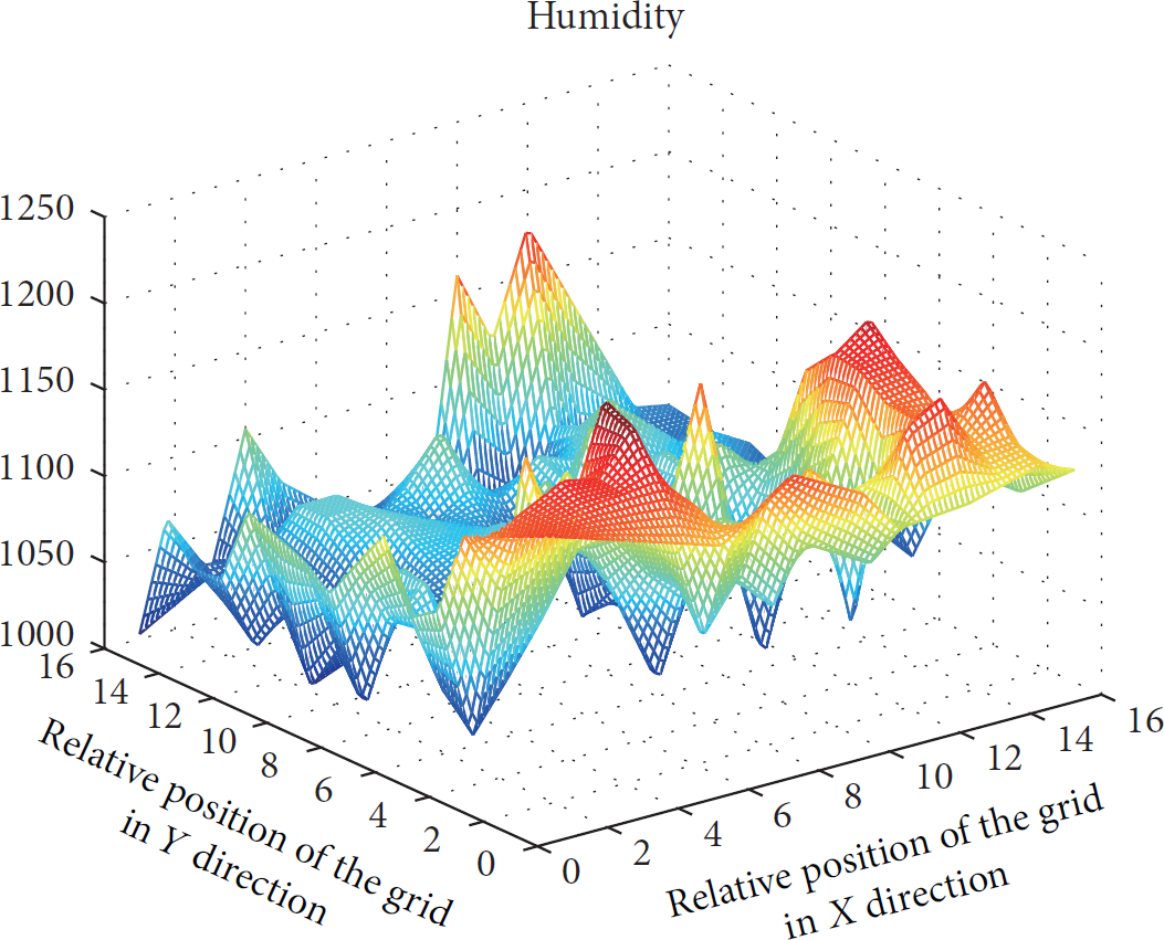
Real monitoring data values displayed in 3D.

Figure 3

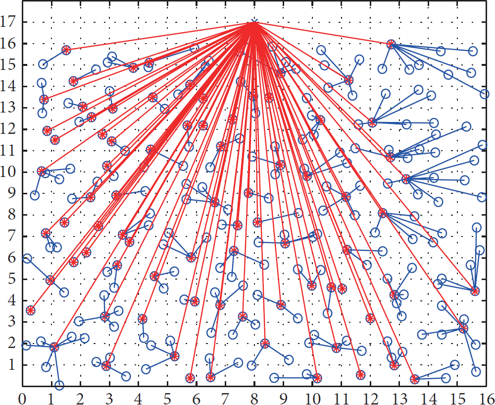
Simulated distributed WSN.

Figure 4

Number of cluster heads versus network lifetime.

Figure 5

Number of cluster heads versus recovery precision.

4.2. Network Lifetime Based on Different Measurement Matrices

Our experimental simulation results show that although the Gaussian random measurement matrix is widely utilized in image processing, it does not have the characteristic of distributed networks and often requires large storage space and high computational complexity. Thus, it is unsuitable for WSNs. The proposed measurement matrix design based on LEACH clustering can effectively prolong the lifetime of WSNs. Figure 6 shows the network's lifetime based on four different methods, namely, traditional LEACH clustering method without CS (LEACH_Method), Gaussian random measurement (Random_Method) [6], measurement based on single-hop routing policy (One_Hop_Method) [17], and our proposed measurement based on LEACH clustering method (CS_LEACH_Method) [18]. Note that One_Hop_Method assumes that all the nodes can send messages to the sink node within one hop. As shown in Figure 4, our solution CS_LEACH_Method is superior to the other methods because of 2 main facts: (1) in both methods of Random_Method and One_Hop_Method, there is large transmission cost because there are no data convergence and compression during the data acquisition; (2) in the method of Gaussian random, there exists higher uncertainty that will lead some nodes unexpectedly to be dead because it fails to consider the nodes' remaining energy while we evenly distribute the energy load among the sensors in the network in the CS_LEACH_Method [18]. We developed a clustering scheme by considering the remaining energy of each node and compressing the data in the head node of each cluster, which, as a result, decreases the number of communication packets and prolongs the lifetime. Thus, in the subsequent data recovery experiments, we employed CS_LEACH_Method to construct the measurement matrix for DAF_CSOR.

Figure 6

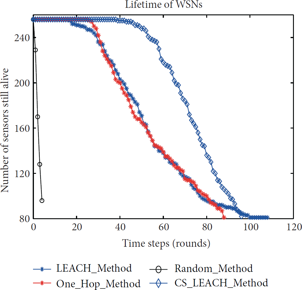
Lifetime of different methods.

4.3. Performance Analysis

The performance of the three recovery methods under the DAF_CSOR framework is shown in Figure 7. The blue marks represent the original signal, and the red ones represent the recovered signal. The three methods exhibit different performances and features because of their different atomic selection strategies and iteration stop conditions. In this section, we present the comparison and analysis of our experimental results and measure the performance of the three recovery methods in terms of running time and relative error.

Figure 7

Performance of different recovery methods.

4.3.1. Error Comparison

We utilized the following formula to calculate the relative recovery error:

$$\begin{array}{c}\text{error}=\frac{{‖X-\tilde{X}‖}_2^2}{{‖X‖}_2^2}=\frac{{\sum }_{i=1}^N{\left(x_i-{\tilde{x}}_i\right)}^2}{{\sum }_{i=1}^N{x}_i^2}.\end{array}$$

(8)

Our data were obtained from 40 selected groups of experiments. Figure 8 shows the recovery errors of three recovery methods under the DAF_CSOR framework and the BCS method in our former research [18]. The errors are approximately 0.05, except for DAF_CSOR_SAMP which is much lower than the others. What contributes to the lower error with the DAF_CSOR_SAMP is its design of backtracking and improvement during the atomic selection procedure. This design makes it has the sparsity-adaptive capability.

Figure 8

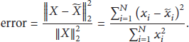
Error of the recovery algorithm under the DAF_CSOR.

The experiments in Figure 9 are conducted under our framework DAF_CSOR. In order to compare with the other framework, we conducted with the 4 different recovery algorithms under the framework with Gaussian random observation matrix. Figure 9 shows the recovery error of four different algorithms. We can see that the recovery algorithm SAMP is inferior to the other 3 recovery algorithms, which have similar result as Figure 8. Overall, DAF_CSOR is superior to Gaussian random and DAF_CSOR_SAMP is more suitable for signal recovery in WSNs when sparsity k is unknown.

Figure 9

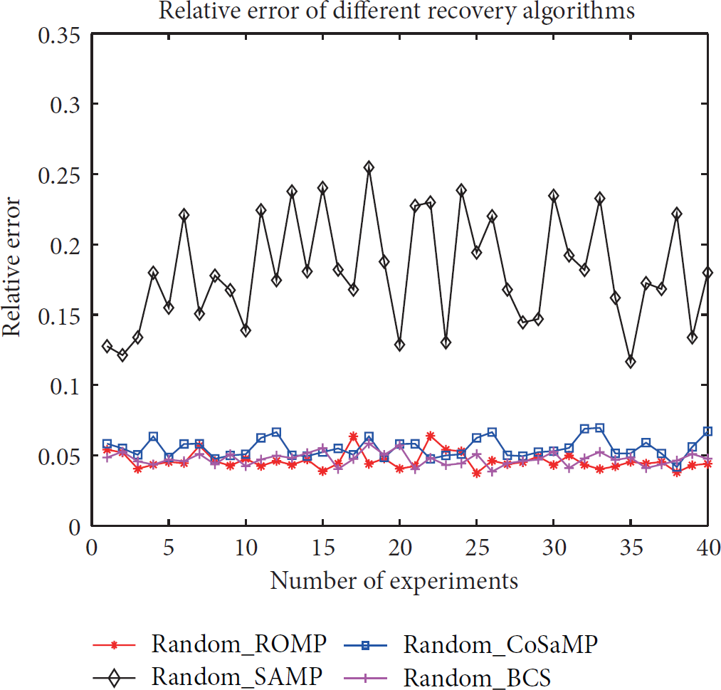
Error of the recovery algorithm under the Gaussian random.

4.3.2. Running Time of the Recovery Algorithms

Figure 10 shows that DAF_CSOR_ROMP is superior in terms of running time. DAF_CSOR_CoSaMP performs excellently in terms of recovery speed. Given that the running time of DAF_CSOR_SAMP is related to the step length, we modified the step length in some of the experiments. As a result, running time changed obviously with different step lengths. The closer the sparsity is to the real value, the shorter the running time is. Network lifetime is unaffected because online recovery is performed in the sink node, which has no energy constraints. Although the speed of DAF_CSOR_SAMP is slightly inferior to that of the other three methods, it is still very fast such that it can meet the needs of WSN applications, such as environmental monitoring.

Figure 10

Running time of the recovery algorithms.

5. Conclusions and Future Work

In this paper, we combined CS theory with WSNs in view of ${\mathcal{l}}_1$ -based convex optimization problem and Gaussian random measurement matrix having limitations when applied to WSNs. We constructed a new measurement matrix according to the spatial correlation among WSN data and conducted WSN data recovery combined with the low-complexity greedy algorithm. The experimental results show that the proposed scheme can effectively extend the lifetime of WSNs. The greedy algorithm is quick and effective in data recovery in WSNs. Meanwhile, the three methods considered exhibit different features because of their different atomic selection strategies and iteration stop conditions. Although DAF_CSOR_ROMP is the fastest in terms of signal recovery, DAF_CSOR_SAMP is relatively more suitable for WSN data recovery research because the sparsity of the natural physical signal is often unknown. In our future work, we will continue to optimize the greedy algorithm-based data recovery method in terms of speed and practicality to make it more suitable for application in real WSN scenarios.