NMCT: A Novel Monte Carlo-Based Tracking Algorithm Using Potential Proximity Information

Abstract

Currently, many services benefit greatly from the availability of accurate tracking. Tracking in wireless sensor networks remains a challenging issue. Most tracking methods often require a large number of anchors and do not take advantage of potential localization information, leading to poor accuracy. To solve this problem, this paper proposes a Novel Monte Carlo-based Tracking (NMCT) algorithm with area-based and neighbor-based filtering, which fully extracts the proximity information embedded in the neighborhood sensing. We describe the entire system design in detail and conduct extensive simulations. The results show that the proposed algorithm outperforms the typical schemes under a wide range of conditions.

1. Introduction

Wireless sensors have been the focus of domestic and international research, and wireless sensor networks (WSNs) represent a revolution of information perception and collection and play a huge role in national defense, space exploration, environmental science, and other fields [1]. A large number of wireless sensors are used in our daily lives and yield a variety of conveniences, with one of the most widely used fields being tracking. People use the received signal strength or other characteristics emitted by the unknown nodes to track and position the target's location. Due to the restrictions of size, power consumption, and other factors of sensors, tracking faces many challenges and requirements. How to retain a balance between the power consumption and the accurate position information becomes the main challenge.

Most tracking methods use a number of seed nodes to receive information from other unknown nodes to estimate the target location [2, 3]. Target tracking is often divided into two steps: location and tracking. Only after getting the target's location we are able to track it. Thus, in some methods, target tracking is target position [4].

Typical location algorithms include the Centroid algorithm [5], DV-Hop (Distance Vector-hop) algorithm [6, 7], Amorphous algorithm [8], and MDS-MAP algorithm [9]. The core idea of the Centroid algorithm is that the geometric centroid of all seed nodes within the communication range of unknown nodes is the estimated location. The Centroid algorithm is simple, but its positioning accuracy is not high [10]. For Amorphous algorithm, each node knows the coordinates of the seed node, and nodes calculate their position based on the received seed location and corresponding hop count. MDS-MAP needs to calculate the shortest path between all nodes, so the communication and computing costs are large, and it is consequently only suitable for short-term and small-scale networks.

However, these methods have not taken the mobility of nodes into consideration and have not taken advantage of the potential localization information [11], which leads to poor accuracy as mobility makes the localization process more difficult and complex. To solve these problems, this paper proposes a Novel Monte Carlo-based Tracking algorithm (NMCT).

In 2004, Hu Lingxuan creatively applied the Monte Carlo Location method to sensor network node localization [12]. The core idea of the Monte Carlo localization algorithm is based on the Bayesian filter position, which represents the possible location of the unknown node as a posterior probability density distribution in the form of a weighted sample set. A particle filter algorithm is a type of suboptimal Bayesian estimation method in nonlinear and non-Gaussian environments [13, 14].

Due to the limited information of an unknown node, the sampling process and filtering process of MCL have to be repeated until it reaches the sample size. As a result, the position accuracy is low.

To fully extract the proximity information embedded in the neighborhood sensing, making the tracking process quicker and the tracking more accurate, our algorithm adds the area-based and neighbor-based filtering to the MCL [15]. Our algorithm has two stages for filtration: prediction and filtering. In the prediction phase, samples are used to describe the posterior probability distribution of unknown nodes. The filtering stage filters out the impossible node samples according to the data sensed by the seed node.

Specifically, our contributions are as follows. (i)

Most of our previous work focuses on investigating the MCL algorithm and its problems. To the best of our knowledge, we construct a complete track framework to address the problems in MCL.

(ii)

We introduce the area-based filtering algorithm and apply it to the MCT algorithm to make the framework more accurate.

(iii)

We use extensive simulation studies to evaluate the performance of the proposed design. The results show that the estimation error is further reduced compared with the existing works.

The rest of the paper is organized as follows. Section 2 discusses related works. Section 3 presents the network model. Section 4 describes the algorithm design. Section 5 presents the simulation results. Section 6 concludes the work.

2. Related Works

Mobile node position systems based on WSN have a wide range of applications in logistics tracking, animal behavior research fields, fire detection, and so forth. Due to the limited capacity of computing and mobility, which will cause measurement noise of nodes, it is much more difficult to achieve high-precision positioning. In 2006, Dynamic Location Schemes (DLS) was proposed to solve the mobile problem in sensor network [16]. It calculated the distance between seeds and unknown node according to the signal strength and estimated the location by the Triangulation [17]. In 2007, Kim and Lee proposed the Mobile Beacon-Assisted Localization (MBAL) algorithm, in which the seed node moves in a predetermined direction while broadcasting signal to unknown node, according to the signal strength and trilateral position method to locate [18]. CDL [19] is a kind of color theory based dynamic location. It uses RGB as the location of sensors. It is a kind of range-free location algorithm. Reference [20] proposes a location algorithm which relies on multiple flight anchor nodes, so it costs high and has to take more security risks.

In 2004, Hu and his colleague firstly applied the particle filter algorithm to the mobile node localization in WSNs and proposed the classic algorithm MCL. The core idea of MCL is using weighted samples to estimate the posterior probability density of the unknown nodes. MCL has achieved very good results in a mobile wireless sensor location. In recent years, domestic and foreign scholars have proposed a variety of improved MCL algorithms. Based on the MCL algorithm, Baggio proposed the Monte Carlo Localization Boxed (MCB) algorithm, which effectively solves the inefficiencies of the traditional MCL algorithm by building an anchor box and sampling box. The MCB algorithm can effectively reduce the estimation error in location, but we have to configure the nodes' ranging parts, which increases the cost of the hardware module [21]. After the MCB algorithm, we proposed Multihop-based Monte Carlo Localization (MMCL), which combines MCL and DV-Hop algorithms and achieves precise positioning when node density is relatively low because the algorithm does not need to know the communication radius of nodes during positioning [22].

Sequential Monte Carlo Localization (SMCL) takes a probabilistic approach so that the network topologies need not be formed beforehand [23]. Mobile-Assisted Monte Carlo Localization (MA-MCL) relies on direct arriver and leaver information from a single mobile-assisted seed [24]. Mobile and Static Sensor Network Localization (MSL) not only takes the location from seeds into account but also uses the location from one-hop and two-hop nonseed neighbors, which facilitates faster and better accuracy than MCL [25].

Most of these algorithms retain the MCL filtering conditions, so the network has higher sensitivity to the number of anchor nodes, the time and space complexity of the algorithm are high, and the position accuracy is not ideal. Thus, this paper advocates an improved MCL algorithm, called NMCT, that is based on the perpendicular bisector zoning method and the PIT algorithm and improves the position accuracy by filtering any sampling area that does not comply with the conditions.

3. Network Model

This section gives an overview of the tracking system, as shown in Figure 1.

Figure 1

Tracking system overview.

The network model is composed of mobile targets with unknown locations and static anchors, we assume time is divided into discrete time units, and the target can move from its previous location. The target's speed and direction are unknown, but we assume the tracking node is aware of the maximum distance it can move in one time unit, which is the maximum velocity $V_{m a x}$ . We also know that the node can emit a signal every T seconds. The anchors are randomly deployed as the unfilled circle shown in Figure 1, and the speed and direction of targets are too random to position.

In this paper, we use the random waypoint model to simulate the motion model. In this model, the node race direction is chosen randomly between 0 and 360 degrees, and the speed is chosen randomly between 0 and $V_{m a x}$ , as the dashed line shows in Figure 1. We assume that there is no bounded area in the network, so the node can move freely, and the movement of each tracking is independent and has no influence on other nodes.

When a mobile node moves into the monitored area of a seed node and when the seed node is in communication range of the target, as the dashed circle shows in Figure 1, the seed node can detect the unknown node and record the signal strength received from it [26]. Due to the different geographic distances between each seed node and target, the signal strength received by different seed nodes is different as well. As the target moves, the signal strength received by the same seed node at different times will also be different. This different signal strength will have an important function in our algorithm.

4. Algorithm Design

Our work is motivated by the MCL algorithm, which is based on the Bayesian filter position. We represent the possible location of the unknown node as a posterior probability density distribution in the form of a weighted sample set. We first present an overview of a three-step design and then describe each step in detail in the following sections.

4.1. Design Overview

Our algorithm also has two stages for filtration: prediction and filtering. Let t be the discrete time and let $t - 1$ be the previous discrete time step. N represents the sample size, and n represents the number of samples remaining after the filtering. The specific steps of the algorithm are as follows.

Step 1 (initialization).

When time = 1, initialize the location of the tracking target.

Step 2.

When time > 1, one has the following:

while ( $n < N$ ), do

(a)

prediction: according to the previous position, predict the node's current possible position;

(b)

sampling: sample a sufficient number of samples M randomly in the possible area;

(c)

filtering: filter the impossible samples according to the observations of the last time step and this time step.

Step 3.

Calculate the position of the unknown node at time = t.

4.2. Algorithm Process

4.2.1. Initialization and Prediction

We assume all nodes have no knowledge of their position. When time = 1, a node has no knowledge of its location, so the initial position is randomly chosen from all of the possible positions. Assume that the locations are represented by $(x, y)$ in a two-dimensional Cartesian space. We sample a sufficient number of samples M randomly in this entire area and calculate the possible location by averaging all of the locations of the possible samples.

The prediction period estimates the present position according to the node position at the last time step. Due to the speed being chosen randomly from between 0 and $V_{m a x}$ , when time > 1, the unknown nodes could be in a circle with a center point $l_{t - 1}$ and a radius of $V_{m a x}$ , and we sample a sufficient number of samples M randomly in this circle ( $l_{t - 1}$ represents the possible location at time $t - 1$ , and the maximum velocity for nodes is $V_{m a x}$ ).

4.2.2. Filtering

The filtering stage filters out the impossible node samples [27]. According to the data sensed by the seed node at time $t - 1$ and time t and the observation of the seed node, we can remove the samples that cannot possibly be the position of the tracking target.

In our network model, the seed nodes receive different signal strengths from the unknown node in this time step and the last time step; for different seed nodes, the signal strength they receive from the same unknown node can be different as well, in that case, we put forward various new filtering conditions to make the sample size more accurate.

(1) Area-Based Filtering Condition. In our network model, every two seed nodes can link to a line and divide the area into two parts; also, every three seed nodes can link into a triangle and divide the samples into the in-triangle part and the out-triangle part. Thus, we employ an area-based approach to perform location estimation by isolating the area into triangular regions after dividing it into near-further parts for different sample nodes. Judging whether the target's location is inside or outside of these triangular regions allows a number of sample nodes to be reduced to narrow down sample nodes' range.

Every two seed nodes can link into a segment, and, theoretically, if the unknown nodes happen to be in the perpendicular bisector (the straight line through the midpoint of a line and perpendicular to this line) of this line, then the signal strength that the two seed nodes received from the unknown node should be equal [28, 29]. Otherwise, the tracking target would be in the left or the right part of the perpendicular bisector [30].

For example, as shown in Figure 2, P and Q are two seed nodes, and l is the perpendicular bisector of PQ. The unknown node A is in area I, and its distance to node P is less than its distance to Q. The unknown node B is in line l, and its distance to node P is the same as its distance to Q. The unknown node C is in area II, and its distance to node P is more than its distance to Q. In wireless sensor networks, the farther away the unknown node is from the seed node, the smaller the received signal strength will be. Thus, for node A, the signal strength that node P can hear from it is higher than the signal strength that node Q received. For node C, the signal strength that node P can hear from it is smaller than the signal strength that node Q received. For node B, the signal strength that node P can hear from it is the same as the signal strength that node Q received in ideal conditions.

Figure 2

Perpendicular bisector zoning method.

In wireless sensor networks, we can connect every two seed nodes that are in the communication range of the unknown node and then obtain many seed pairs. According to the perpendicular bisector zoning method above, for each pair of seed nodes, we can compare the signal strength that they received from the same unknown node and then judge which seed node the unknown node is closer to and which area of the perpendicular bisector it could be in. Through connecting all the seed pairs and judging the possible area where the unknown node could be, the impossible samples are gradually reduced according to the intersection area of this possible area.

After dividing the area into the near-further part, we employ a proposition to isolate the area into triangular regions to make the possible area more accurate. Our proposition is similar to the Point-In-Triangulation (PIT) Test [31], but much easier than it because of the following reasons.

Firstly, according to the PIT algorithm, in the actual test, we often find the InToOut errors and OutToIn error, which just judge the node inside the triangle wrong and judge them outside and locate those outside the triangle wrong and judge them inside [32], so the original PIT is not perfect.

Secondly, in our network model, the speed and direction of a node are unknown, so we cannot do like the PIT algorithm that goes through all of the directions of the unknown node to judge whether there is a direction to make judgment; we only have the information of the position of the unknown node at this time step and the last time step, so we can only determine whether, at this moment, the node is outside the triangle or not, according to these two pieces of information.

Thus, in this paper, as the speed and direction of the tracking node are unknown and the seed nodes are randomly distributed, according to the PIT algorithm, we can randomly select three seed nodes in the communication range of the unknown node, $A (x_{a}, y_{a})$ , $B {(x}_{b,} y_{b})$ , and $C (x_{c}, y_{c})$ and make a triangle with these dots, △ABC. We can then judge whether the unknown node is in triangle △ABC or not according to the following proposition.

If the signal strength received by the same seed node at the last time step is larger than that received at this time, then the sample node is outside the triangle. The following are the different conditions in our network model.

As shown in Figure 3, the tracking target moves from the last time step to this time step in reality. In order to judge the target location at this time step, we have to utilize the information at last time step. Thus, we define a logic direction and take it as the move direction, which is the opposite with actual path.

Figure 3

Different conditions in the triangle algorithm.

As shown in Figure 3(a), if the node moves from this time step to the last time step along the logic direction, it will be far away from seed nodes A, B, and C. According to the PIT, this means there is a direction that makes the distance between the node and three dots (A, B, and C) get longer. Theoretically, the node can be regarded as out of △ABC at this time step. However, due to the typical InToOut error shown in Figure 3(c), this conclusion does not always hold.

In the same way, if the node moves from this time step to the last time step along the logic direction as shown in Figures 3(b) and 3(d), it will make the “new” position become closer to seed nodes A, B, and C. According to the PIT principle, this means that there is a direction that makes the distance between the node and three dots get shorter, and there are no InToOut errors or OutToIn error in this situation, so we can conclude that the node is out of △ABC at this time step. If the target is being far away from the seed nodes, the signal strength that A, B, and C received at this time step should be smaller than that at the last time step. Hence, we can obtain the below proposition: if the signal the same seed node received at the last time step is larger than that received at this time step, the sample node is outside the triangle.

Thus, using all of the triangles which are made by the seed nodes, we can judge the triangular area that the nodes are certainly not in and then discard all of the samples located in the corresponding area.

(2) Neighbor-Based Filtering Condition. To make the filtering results more accurate, we further propose a neighbor-based filtering condition.

Specifically, each predicted position within the communication of the seed node can send broadcasts to the seed node at the current time t. If the seed cannot receive the broadcast from a predicted position, it indicates that this indicated position should be discarded. Here, we mainly rely on the one-hop and two-hop seed node information to filter the impossible samples.

A one-hop seed node is a seed node that can directly listen to the unknown node, while two-hop seed node refers to the seed node that cannot listen to the unknown node directly, but they can hear a one-hop seed node. It means the distance between the sample and the two-hop seed nodes is between r and $2 r$ . Assuming that S represents a one-hop heard node and T represents two-hop heard nodes, the filter conditions are

\begin{matrix} F i l t e r (l) = (\forall s \in S, d (l, s) \leq r) \cup (\forall s \in T, r < d (l, s) \leq 2 r), \end{matrix}

(1)

in which

d (l, s)

represents the distance between sample l and node s, and r represents the node's range radio. Only when the filter condition is satisfied the prediction of the position of the unknown node is possible.

Thus, based on the one-hop and two-hop message from the sample node, we can analyze each sample in the sample areas to find whether they meet the filtering conditions and then abandon the impossible samples.

4.2.3. Resampling and Calculation

After filtering, the remaining samples may be minimal, so we need to perform the resampling operation for supplementing the samples. The algorithm repeats the prediction stage and filter stage until enough samples are collected.

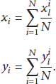
After the resample process, we calculate the position of the unknown node at time t, as in formulas (2), in which we assume locations are $(x, y)$ positions in a two-dimensional Cartesian space:

\begin{matrix} x_{i} = \sum_{i = 1}^{N} \frac{x_{l}^{i}}{N} \\ y_{i} = \sum_{i = 1}^{N} \frac{y_{l}^{i}}{N} . \end{matrix}

(2)

4.3. Specific Situation

Without loss of generality, we give the distribution of the seed node and target movement scenario shown in Figure 4 for describing the filtering process. The filled black circle represents the position of the target at last time step, while the filled red circle represents the actual target position at the current time step. In addition, the unfilled white circles represent the sample points, and the filled triangles represent the seed nodes, which is A, B, C, and E. Finally, the solid circles with different color denote the corresponding communication radius of nodes.

Figure 4

Specific situation.

Based on the proposed movement model and prediction method, we first pick up a number of samples randomly from the circle that takes the location at last time step as the center point and $V_{m a x}$ as the radius. 17 samples are chosen in this scenario. As shown in Figure 4, when seed nodes A, B, and C receive the signal from target, they begin to perform the filtering operation.

According to the area-based filtering condition, we then compare the signal strength received by every two seed nodes in the communication range of the targets. For example, we connect the seed nodes A and B. Let $l_{1}$ be the perpendicular bisector of the segment AB. By comparing the signal strength they receive from the target, we can conclude that the target gets closer to seed B. Hence, samples 12, 13, 14, 15, 16, and 17 can be abandoned. Similarly, from the signal strength comparison between nodes A and C, we can discard samples 1, 2 and 3. For nodes B and C, we can further throw away samples 4 and 5.

After using the perpendicular bisector zoning method, we further use APIT to discard more samples. For seed nodes A, B, and C, the strength they received from the target at this time is smaller than that of the last time. According to our algorithm, we can make sure the target is out of the triangle that is constructed by the seed nodes A, B, and C, thus we discard sample 9 that is inside △ABC.

Through the above filtering, there are only samples 6, 7, 8, 10, and 11 remained. According to the hop-based filtering condition, for the one-hop seed nodes like the seed node B, the distance between node B and target must be within the communication range (R) of the target, so all the samples whose distance to seed B are longer than R should be discarded. Thus, samples 7 and 10 are abandoned. For the two-hop seed node and taking node E as an example, the distance between node E and the target must be between R and $2 R$ , so we discard sample 8. After performing all the filter process, there are only samples 6 and 10 left. Finally, we calculate the average location of the remaining samples as the estimated location at time step t.

5. Evaluation

In this section, we compare the performance of the proposed algorithm with the Centroid algorithm, Amorphous algorithm, and original MCL algorithm. We mainly study the impact of time, node speed, seed density, sample number, and radio range irregularity [33] on system performance.

5.1. Simulation Parameters

Similar to the original MCL algorithm, sensor nodes are randomly distributed in a 500 m × 500 m rectangular region for all experiments. We use the same transmission range, r, of 50 m for both nodes and seeds. We also use the random waypoint [34] model to make sure the unknown nodes can vary their speed during different movements.

The speed of the node is randomly chosen from $[V_{m i n}, V_{m a x}]$ and the node density ( $n_{d}$ ) is the average number of nodes in the one-hop transmission range. It is set to be 10 in the simulations. We also study the effects of varying $n_{d}$ in Section 5.2.3. In addition, N is used to represent the number of samples maintained. For all of the other simulations, we use $N = 50$ .

5.2. Simulation Results

5.2.1. Accuracy

In this section, we compare NMCT algorithm with original MCL algorithm, Centroid algorithm, and Amorphous algorithm. We also simulate the impact of time on the accuracy of NMCT.

Figure 5 shows a comparison of the accuracy of different algorithms. From the figure, we can see that the Amorphous algorithm initially performs the best and has the lowest estimation error. However, NMCT algorithm exceeds Amorphous algorithm and continues to have the lowest error after 10 steps. From an overall perspective of the Centroid, Amorphous, MCL, and NMCT algorithms, NMCT performs the best and Centroid performs the worst. The Centroid and Amorphous localization techniques do not exploit past information, so they do not improve over time. Since MCL and NMCT update the estimate position according to the latest results from the observed phase, the estimation errors of MCL and NMCT both decrease quickly as time passes. In particular, NMCT decreases quicker.

Figure 5

Accuracy comparison.

5.2.2. Node Speed

In the second simulation, we study the impact of node speed on the estimation error. As shown in Figure 6, because the Centroid and Amorphous algorithms have not considered the mobility of nodes, the speed of nodes has little impact on them.

Figure 6

Impact of node speed on different algorithms.

From Figure 6, we can see that the estimation error decreases for MCL and NMCT when the node speed increases between $0.2 r$ and $0.4 r$ . But the estimation error increases while $v_{m a x}$ is larger than $0.4 r$ . That is because node speed impacts the localization process in two ways. At the beginning, faster movement leads to more new observations in each time step, and hence more impossible locations can be filtered, which makes the predicted locations more accurate. On the other hand, the increased speed makes the predicted locations less accurate since the next possible locations fall into a larger region. That is to say, the increasing speed brings too much uncertainty and the obtained new observations cannot reduce the uncertainty, leading to a poor accuracy. In addition, Figure 7 shows the location convergence of NMCT. At the beginning, the estimate error decreases dramatically because new observations are incorporated. As time goes on, the estimate error keeps some balance.

Figure 7

Impact of node speed on NMCT.

5.2.3. Seed Density

We conduct the third simulation to study the impact of seed density on the estimation error. Obviously, more seeds can improve the tracking accuracy. More seeds can receive the announcements and provide more observations. Hence, more samples can be reduced and abandoned, although this will also require more hardware resources.

Figure 8 shows the impact of seed density on location accuracy. For Amorphous, because each node receives the propagated messages from all seeds in the network, the estimation error does not improve much when there are a sufficient number of seeds. For the MCL and NMCT algorithms, the estimation error is very high when the seed density is very low, but it drops rapidly as the seed density increases. When the seed density rises to approximately 3.5, the estimation error is gradually stable. Similar to NMCT, Centroid algorithm improves obviously as the seed density increases, but NMCT is much more accurate.

Figure 8

Impact of seed density on different algorithms.

Figure 9 shows the impact of seed density with different node speeds. Three scenarios with different node speed are simulated. As the seed density increases, the nodes with smaller speed have the quicker reduction of the estimation errors. When the seed density continues to increase, the curves become flat for all the scenarios.

Figure 9

Impact of seed density with different node speeds.

5.2.4. Number of Samples

This simulation studies the impact of sample size on the accuracy. We increase the sample size from 1 to 500.

More samples can make the tracking more accurate, but this requires additional memory. There should be a trade-off between the accuracy and resources. So, we conduct this simulation. As shown in Figure 10, the estimation error is very high and the position is very inaccurate when the sample size is very small. As the sample size increases, the estimation error drops quickly. When the sample size is larger than 100, the estimation error of MCL and NMCT becomes relatively stable. Nevertheless, NMTC still performs better than MCL.

Figure 10

Impact of sample size.

5.2.5. Irregularity

This simulation studies the impact of radio range irregularity on estimation error. In a practical application, the radio communication range is usually irregular [35], so it is necessary to evaluate this parameter. Unlike the prefect circles assumed in our previous description, the measured reception distance of radios can vary substantially with environmental conditions and antenna irregularities. In the simulation, we change the radio range irregularity from 0 to 50%, as shown in Figure 11. For the Amorphous algorithm, the estimation error significantly increases when the irregularity increases. This is because the ranging estimate is from the propagation of hop count, and it always selects the minimal hop count. Hence, irregular radio transmissions will have an accumulating effect on the ranging error in multiple hops. However, for the MCL and Centroid algorithms, the range irregularity has little impact on the performance of NMCT. And it is noted that the accuracy of NMCT will still be better than that of MCL with the increasing of the irregularity.

Figure 11

Impact of irregularity.

6. Conclusion

In this paper, to solve the problem of the sampling area of the MCL algorithm being too large and to improve the accuracy and effectiveness of MCL, we combine the area-based filtering algorithm with the MCL algorithm and make use of the signal strength received from the unknown nodes to exclude the areas that unknown nodes do not exist in. As the results show, NMCT can improve the accuracy and efficiency of positioning in different conditions, even when the network is highly irregular or the sample size is low. Many issues remain to be solved in future networks, including how to further reduce the impossible sampling area, how different motion models will affect the simulation, and how to improve the security of the network.

Footnotes

Conflict of Interests

The authors declare that there is no conflict of interests regarding the publication of this paper.

Acknowledgments

This work was supported by the Fundamental Research Funds for the Department of Science and Technology Project of Jiangsu Province under Grant BY2014028-09, the Postdoctoral Science Foundation of China under Grant 2014M561727, Department of Transportation Research Project of Zhejiang Province under Grant 2014T25, and the National Natural Science Foundation of China under Grant 51404258.

References

Song

The application of WSN technology in the space location system

Proceedings of the 4th International Congress on Image and Signal Processing (CISP ′11)

October 2011

Shanghai, China

633 636

10.1109/CISP.2011.6100316

Zhang

Liu

Wang

Cao

Min

Accurate range-free localization for anisotropic wireless sensor networks

ACM Transactions on Sensor Network 2015 11 3, article 51

Gao

Chen

Suboptimal filtering of networked discrete-time systems with random observation losses

Mathematical Problems in Engineering 2014 2014 8

151836

10.1155/2014/151836

MR3198446

2-s2.0-84899986546

El Assaf

Zaidi

Affes

Kandil

Range-free localization algorithm for anisotropic wireless sensor networks

Proceedings of the 80th IEEE Vehicular Technology Conference (VTC Fall ′14)

September 2014

Vancouver, Canada

IEEE

1 5

10.1109/VTCFall.2014.6966149

Girod

Estrin

Robust range estimation using acoustic and multimodal sensing

Proceedings of the IEEE/RSJ International Conference on Intelligent Robots and Systems (IROS ′01)

October 2001

Maui, Hawaii, USA

1312 1320

Niculescu

Nath

Ad hoc positioning system (APS)

Proceedings of the IEEE Global Telecommunications Conference (GLOBECOM ′01)

November 2001

San Antonio, Tex, USA

2926 2931

10.1109/GLOCOM.2001.965964

Niculescu

Nath

DV based positioning in ad hoc networks

Telecommunication Systems 2003 22 1 267 280

10.1023/a:1023403323460

2-s2.0-0038703640

Nagpal

Organizing a Global Coordinate System from Local Information on an Amorphous Computer 1999

Cambridge, Mass, USA

MIT Computer Science and Artificial Intelligence Laboratory

Shang

Ruml

Zhang

Localization from mere connectivity

Proceedings of 4th ACM Symposium on Mobile Ad-Hoc Networking and Computing

June 2003

Annapolis, Md, USA

201 212

10.

Bulusu

Heidemann

Estrin

Density adaptive algorithms for beacon placement in wireless sensor networks

Proceedings of the International Conference on Distributed Computing Systems (ICDCS ′01)

April 2001

489 498

11.

Bai

Mobile sensor deployment optimization for k-coverage in wireless sensor networks with a limited mobility model

IEEE Technical Review 2010 27 2 124 138

12.

Evans

Localization for mobile sensor network

Proceedings of the 10th Annual International Conference on Mobile Computing and Networking (MobiCom ′04)

September 2004

Philadelphia, Pa, USA

45 57

13.

Dellaert

Fox

Burgard

Thrun

Monte Carlo localization for mobile robots

Proceedings of the 1999 IEEE International Conference on Robotics and Automation (ICRA ′99)

May 1999

Detroit, Mich, USA

IEEE

1322 1328

2-s2.0-0032632827

14.

Thrun

Fox

Burgard

Dellaert

Robust Monte Carlo localization for mobile robots

Artificial Intelligence 2001 128 1-2 99 141

10.1016/s0004-3702(01)00069-8

2-s2.0-0035336711

15.

Huang

J.-F.

Chang

G.-Y.

Chen

G.-H.

A historical-beacon-aided localization algorithm for mobile sensor networks

IEEE Transactions on Mobile Computing 2015 14 6 1109 1122

10.1109/tmc.2014.2346777

16.

Chen

Han

Q. S.

A viable localization scheme for dynamic wireless sensor networks

Proceedings of the 1st International Multi-Symposiums on Computer and Computational Science

June 2006

Hanzhou, China

587 593

10.1109/IMSCCS.2006.174

17.

York

Pack

Comparative study on time-varying target localization methods using multiple unmanned aerial vehicles: kalman estimation and triangulation techniques

Proceedings of the IEEE International Conference on Networking, Sensing and Control (ICNSC ′05)

March 2005

Tucson, Ariz, USA

IEEE

305 310

10.1109/icnsc.2005.1461206

2-s2.0-33745139454

18.

Kim

Lee

MBAL: a mobile beacon-assisted localization scheme for wireless sensor networks

Proceedings of the 16th International Conference on Computer Communications and Networks

August 2007

Honolulu, Hawaii, USA

57 62

10.1109/ICCCN.2007.4317797

19.

Chang

Wang

Hsieh

Y. L.

Color-theory-based dynamic localization in mobile wireless sensor networks

Proceedings of the 1st Workshop on Wireless Ad Hoc Sensor Networks

2005

73 78

20.

C.-H.

Ssu

K.-F.

Sensor position determination with flying anchors in three-dimensional wireless sensor networks

IEEE Transactions on Mobile Computing 2008 7 9 1184 1197

10.1109/TMC.2008.39

2-s2.0-48149100746

21.

Baggio

Langendoen

Monte-Carlo localization for mobile wirelesss sensor networks

Mobile Ad-Hoc and Sensor Networks 2006 6 5 718 733

22.

Yang

Cha

Multi-hop-based Monte Carlo localization for mobile sensor networks

Proceedings of the 4th Annual IEEE Communications Society Conference on Sensor, Mesh and Ad Hoc Communications and Networks (SECON ′07)

June 2007

San Diego, Calif, USA

IEEE

163 171

10.1109/sahcn.2007.4292828

2-s2.0-48049108498

23.

Wang

Zhu

Sequential Monte Carlo localization in mobile sensor networks

Wireless Networks 2009 15 4 481 495

10.1007/s11276-007-0064-3

2-s2.0-62249210277

24.

Teng

Zheng

Dong

MA-MCL: mobile-assisted Monte Carlo localization for wireless sensor networks

International Journal of Distributed Sensor Networks 2011 2011 8

671814

10.1155/2011/671814

2-s2.0-80052669862

25.

Rudafshani

Datta

Localization in wireless sensor networks

Proceedings of the 6th International Conference on Information Processing in Sensor Networks (IPSN ′07)

April 2007

ACM

51 60

10.1145/1236360.1236368

2-s2.0-35348855583

26.

Kanamaru

Suzuki

Asahi

Watanabe

Proposal for a wireless sensor network visualization system using location estimation technology

Proceedings of the 7th International Conference on Mobile Computing and Ubiquitous Networking (ICMU ′14)

January 2014

Singapore

111 116

10.1109/icmu.2014.6799080

2-s2.0-84900010173

27.

Chen

Gao

Huang

Modified extended Kalman filtering for tracking with insufficient and intermittent observations

Mathematical Problems in Engineering 2015 2015 9

981727

10.1155/2015/981727

MR3407174

28.

Chen

Gao

Huang

SSL: signal similarity-based localization for ocean sensor networks

Sensors 2015 15 12 29702 29720

10.3390/s151129702

29.

Yuanchao

Peng

TOC: localizing wireless rechargeable sensors with time of charge

ACM Transactions on sensor Networks 2015 11 3

30.

Bocca

Kaltiokallio

Patwari

Venkatasubramanian

Multiple target tracking with rf sensor networks

IEEE Transactions on Mobile Computing 2014 13 8 1787 1800

10.1109/TMC.2013.92

2-s2.0-84904159759

31.

Girod

Estrin

Robust range estimation using acoustic and multimodal sensing

Proceedings of the IEEE/RSJ International Conference on Intelligent Robots and Systems

November 2001

Maui, Hawaii, USA

1312 1320

2-s2.0-0035560043

32.

Huang

Blum

B. M.

Stankovic

J. A.

Abdelzaher

Range-free localization schemes for large scale sensor networks

Proceedings of the 9th Annual International Conference on Mobile Computing and Networking

October 2003

ACM

81 95

2-s2.0-1542329081

33.

Adnan

Datta

MacLean

Efficient and accurate sensor network localization

Personal and Ubiquitous Computing 2014 18 4 821 833

10.1007/s00779-013-0692-9

2-s2.0-84897430463

34.

Camp

Boleng

Davies

A survey of mobility models for Ad Hoc networks research

Wireless Communications and Mobile Computing 2002 2 5 483 502

10.1002/wcm.72

35.

Zhou

Krishnamurthy

Stankovic

J. A.

Impact of radio irregularity on wireless sensor networks

Proceedings of the 2nd International Conference on Mobile Systems, Applications and Services (MobiSys ′04)

June 2004

Boston, Mass, USA

125 138

2-s2.0-4544263123