Sage Journals: Discover world-class research

Abstract

We investigate a centralized wind farm controller which runs periodically. The controller attempts to reduce the damage a wind turbine sustains during operation by estimating fatigue based on the wind turbine state. The investigation focuses on the impact of information access and communication networks on the controller performance. We start by investigating the effects of a communication network that introduces delays in the information access for the central controller. The control performance as measured by accumulated fatigue is shown to be significantly impacted by communication delays and also by the choice of the time instances at which sensor information is accessed. In order to optimize the latter, we introduce an information quality metric and a mathematical model based on Markov chains, which are compared performance-wise to a heuristic approach for finding this parameter. This information quality metric is called mismatch probability, mmPr, and is used to express quantitatively the information accuracy in a given scenario. Lastly, measurements of different communication technologies have been performed in order to carry out the analysis in a practically relevant scenario with respect to the communication network delays. These measurements are done in regard to packet loss and communication delays, and the simulations are rerun using either the traces from the measurements or scenarios constructed from the delay parameters.

1. Introduction

Over the last few years, we have seen an increase in deployment of renewable energy generation. Due to increased deployment and the fluctuating nature of renewable power generation, there is a greater need for controlling the balance between energy consumption and production by means of Smart Grid deployments. One large contributor to renewable generation is wind farms. Controlling a wind farm can be done from a central controller which harmonizes the wind farm's power generation by sending set-points to each wind turbine; thus, a control is performed via a communication network. This way, a central controller ensures that each wind turbine produces the required amount of power. For deployment of the wind farm communication network, it is possible to use different technologies; however, each technology has different behavior; hence, it is important to analyze the impact of these communication technologies on the controller's performance.

In this paper, we consider a central wind farm controller gathering information from wind turbines distributed over an area. We analyze control performance under communication network conditions and determine which parameters of the information access have a strong impact. In order to optimize the parameter, we determine an information quality model, expressing quantitatively the information accuracy as difference between the value used by the controller and the real physical value. This information access model, therefore, needs to include information dynamics, which we obtain empirically from a simulation of the system. In order to perform the analysis in a practically relevant scenario with respect to communication delays, we perform measurements of different communication technologies, where we measure packet loss and delays and use these measurements when simulating the wind farm controller. The comparison of the simulation results of control performance metrics provides a quantitative basis for the suitability of communication technologies for this distributed control scenario.

In recent years, attempts have been made to create Smart Grid test-beds that integrate electrical assets (or their models) with communication technologies (or communication network simulators) in order to study interdependencies between the cyberphysical systems [1]. One such example is [2] which demonstrates a test-bed that includes wired and wireless technologies. It is based on ethernet and ZigBee networks. Reference [3] introduces a cognitive radio network in a Smart Grid test-bed (specifically a microgrid), with the main focus on the security of the Smart Grid. In [4], Zigbee is used as the communication technology and is implemented in an office environment with the goal of optimizing the energy costs for the offices connected to the Smart Grid. Measurements of WLAN technology in other scenarios confirm the order of magnitude of the observed delays in our experiments. However, in the presence of stronger cross-traffic, the shape of the delay distribution will change; see [5]. Reference [6] details different communication technologies available for wind farm communication; among these are WLAN and ethernet based solutions. Another communication technology for a wind farm is fiber optics, as described in [7]. Unlike previous work that analyzed communication technologies for wind farms, our methodology is based on measurements obtained from real communication networks in a scaled down manner compared to the real environment. Subsequently, we use the measurement results by plugging the traces into a cosimulation framework which is similar to the framework used in [8].

The use of sensor information in distributed systems is subject to two types of inaccuracies: measurement errors at the sensor may propagate through the whole computation chain; see, for example, [9] for work characterizing such errors and their impact. For distributed real-time systems, a second cause of inaccuracies requires attention: while the sensor data is being transmitted and processed, the actual physical value changes so that it deviates from the value used in the processing. In this paper, we focus on the second aspect and utilize an information quality metric called mismatch probability (mmPr). This metric and mathematical model for certain base cases was introduced first in [10]. mmPr considers the aspect of real-time information access, capturing impact of access delays and access strategies on information accuracy in a distributed system. So far, this metric has been used in the following context: (i) in [11], mmPr was used in context subscription management systems for effective configuration of context access strategies in order to maximize the reliability of context information and (ii) in [12], the metric was used to find optimal location-based relay policies in mobile networks. In this paper, we investigate whether optimization of the information quality is a means of improving the control performance of the hierarchical wind farm controller.

The work in this paper builds upon the conference publications in [13–15]. Compared to these conference papers, additional results are included, showing the following new aspects: (1) the simulation results use longer traces and drop the transient phase of the simulation; that way, better statistical significance of the results is achieved; (2) the communication network structure is now hierarchical and performance measurements from a CAN network simulation are used to characterize the impact of this hierarchical structure; and (3) the analytic model from [14] for the information quality metric has been newly developed to now explicitly distinguish control actions and system evolution without control. It now fully captures the qualitative behavior of the corresponding simulations.

2. System Overview

This paper considers a system consisting of a central controller, communicating with N wind turbines over a communication network, with each wind turbine containing K sensors. There is a bidirectional information flow consisting of sensor measurements from the sensors to the central controller and set-points from the controller to the wind turbine. The architecture of the system is shown in Figure 1 and explained further in Section 2.1.

Figure 1

Overview of the communication architecture.

The central controller has the objective to follow a set-point for the wind farm's power generation while reducing the fatigue a wind turbine experiences in order to prolong the lifetime of the wind turbine. The central controller should ensure that each wind turbine in the farm produces a certain level of power to ensure that the entire wind farm reaches the given set-point for the wind farm, motivating the central control architecture in Figure 1. The sensors send information regarding the state of the wind turbine to the central controller. The central controller uses the sensor values and its internal state to compute set-points for the wind turbine. These set-points are then forwarded to the wind turbine, where the local controller uses them to adjust the wind turbine. An overview of this scenario can be seen in Figure 1, where the grayed boxes denote places that introduce delay in the information flow. In this paper, we assume that the central controller is executing periodically with a fixed deterministic period of duration $T_{s}$ .

2.1. Communication Network Architecture

The end-to-end communication path between a sensor and the central controller consists of two communication networks, which can be seen in Figure 1, with conceptually different properties, a Sensor Network and an Access Network. The Sensor Network is an internal communication network on the wind turbine and can be implemented by different communication technologies, for example, a fieldbus. It handles the communication between the sensors on the wind turbine and contains a gateway that handles communication from the wind turbine to the central controller. The Access Network is the network between a wind turbine and the central controller and varies in size based on the size of the wind farm. An off-shore wind farm can have lengths of over 20 km with hundreds of wind turbines, which must be covered by the given communication network. The network could be implemented by technologies such as 2G, 3G, WLAN, fiber optics, or PLC.

Cellular networks are already deployed in many regions and hence can be used without further infrastructure. Whether 2G or 3G fulfils the requirements of this scenario is part of the analysis. WLAN is an off-the-shelf technology readily available and covering a few hundreds of meters which could support wind farms in a geographically smaller area. PLC in principal could be interesting, as the central controller and the wind turbine controller may be connected via power lines, which would mean that except the PLC modems no additional infrastructure is needed. However, unlike the hard-wired communication infrastructure, PLC and WiFi technologies can have additional drawbacks impacting their reliability. For instance, PLC communication is not possible if the power line is cut, while WiFi technology has a shared spectrum, possibly reducing the performance. The fiber optics gives the best QoS but may not be available to already deployed wind farms and may require additional costs to implement.

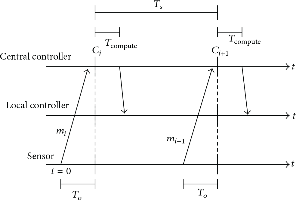
Figure 2 depicts a message sequence diagram of a control period with message delays. The figure shows that during a given control period the central controller will calculate a set-point for the wind turbine. The set-point will be sent to the wind turbine, which will then act upon it. At some point during the control period, defined by the value $T_{o}$ , denoting the offset time prior to control computation $C_{i}$ , the sensor will take a reading and will send it via the Sensor Network to the gateway that forwards the sensor reading via the Access Network to the central controller. For simplicity, Figure 2 only shows the communication endpoints; the delays indicated by the tilt of the messages are end-to-end delays.

Figure 2

Message sequence diagram between the sensor and central controller for a single wind turbine.

The information access strategy, thus, is that the controller sends one control set-point during each control period, and the sensor sends a measurement once each control period, determined by the offset $T_{o}$ with sensor readings. The gateway will forward any packet it gets from the sensors immediately to the controller and is thus not shown in this figure.

2.2. Controller Design

The central controller aims to reduce the fatigue load of the shaft in the wind turbine. It does this while tracking a desired power reference. To achieve this, the central controller requires an input from a fatigue estimator. This estimator requires sensor measurements of the wind turbine, which are the physical measurements of torque, as well as the angle rotation of the wind turbine. These measurements are run through different hysteresis relays with different weights. For details on estimator synthesis and the controller, see [16].

The control scheme without network effects is depicted in Figure 3. In this paper, we assume that the fatigue estimator (F) and the controller (C) are colocated in a central controller. This controller describes the procedures for an individual wind turbine, while the same procedure, with coordination on the generation share of each wind turbine, is applied for the whole farm, which requires a centralized controller. For control performance, we later analyze a single wind turbine as we focus on the fatigue as the KPI describing control performance, while the communication scenario is shaped by the whole wind farm.

Figure 3

Centralized controller scheme without network effects.

The controller cycle, $T_{s}$ , is determined by the design of the controller and is in this scenario set to 150 ms and cannot easily be changed. The central controller is assumed to have a 50 ms computation time. We consider a total of 30 wind turbines, each with $3$ sensors, in the wind farm, which constitutes a small to medium sized wind farm.

3. Controller Performance under Communication Network

We start by investigating if a delay in the communication network and a specific access strategy have an impact on the performance of the central controller. To do this, a cosimulation framework has been developed, in which MATLAB is used to simulate the wind turbine controller, and OMNeT++ is used to simulate the communication network. An interface has been developed for the controller, allowing it to interact with the OMNeT++ simulation. The OMNeT++ part of the simulation is in charge of timing requirements, that is, when to simulate the controller, wind turbine, or fatigue estimator, and is thus in charge of handling the information access strategies. In the simulations, time is handled by an internal clock, ensuring perfect synchronization between all modules in the simulation. The wind turbine is modelled by the differential equation linearised around a chosen operating point. Consider

\begin{matrix} X (t + 1) = A_{d} \cdot X (t) + B_{d} \cdot U (t) + E_{d} \cdot V (t), \end{matrix}

(1)

where X is the state of the wind turbine, U is the control set-point, and V is the wind, which is real wind data. How these interact is determined by the matrices

A_{d}

B_{d}

, and

E_{d}

, and we refer to [16] for details for determining these matrices. Here, we let t be the discretized time.

3.1. Scenario Parameters

Some assumptions regarding the controller and its physical representation are taken in order to simplify the simulations. It is assumed that there will be end-to-end communication delays in the communication network due to propagation delay, queues, and computation delays. We also assume that the controller and the sensors have perfect clock synchronization. In regard to the controller, it is assumed that both the fatigue estimator and the computation of the wind turbine set-points have an internal computation delay, as summarized in the value given in Table 1. This computation delay is used by the fatigue estimator to estimate the fatigue of the wind turbine based on the wind turbine state and by the controller to calculate a new set-point based on the output of the fatigue estimator. At any given time, there is a change in the wind turbine state; it is assumed that the sensors are able to get a reading of this instantly. An example of this could be a new control set-point or a change in wind speed. The wind turbine itself is assumed to act on a set-point as soon as it is received, and we assume that this is done instantly and that the change has an impact on the state of the wind turbine instantly. The wind data which have been used in the simulations have been downloaded from [17]. The wind data used have a measurement every 12.5 ms, leading to 12 samples per control period.

Table 1

Parameters on the overall wind farm topology and parameters for the control execution.

Controller cycle, $T_{s}$	150 ms
Controller computation delay	50 ms
Number of wind turbines	1
Number of sensors	3

Table 1 details the relevant parameters for the simulation scenario.

We start by investigating the performance of the central controller over increasing delays. We assumed a periodic access strategy as described in Section 2.1, where the offset is set to 75 ms. As we are mainly interested in the impact of the nonideal networks in the access to the sensor information, we assume, for the downstream communication from central controller to wind turbine, a constant 1 ms delay. For the “upstream” end-to-end communication between sensor and controller, we assume a shifted exponential distribution, with a fixed minimum of 1 ms and we change the exponential rate in order to change the mean of the upstream delays.

Figure 4 depicts the accumulated damage over increasing total mean delays, with the dashed lines depicting the 95% confidence interval. It shows that, as the average delay increases, the accumulated damage increases, and thus the performance of the controller decreases. For further analysis in this section, we focus on the parameter regime of delays that are well below the control period duration of 150 ms. We, therefore, choose to use a shifted exponential distribution with a mean of 31 ms in the remainder of this section. We next attempt to determine the effect of different offsets on the performance of the controller.

Figure 4

The accumulated damage of the wind turbine over increasing delays with 95% confidence intervals; the X-axis denotes the mean of the upstream end-to-end delays between sensors and central controller.

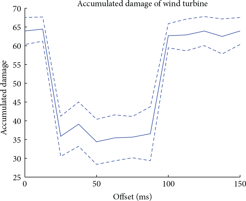
The results in Figure 5 show that the accumulated damage of the wind turbine decreases as the offset increases, until it reaches a minimum at $T_{o} \approx 90$ ms. A consequence of a small choice of $T_{o}$ is that a large fraction of the update message from the sensors does not arrive in time to be considered for the control computation. As a consequence, the controller would use the “old” value from the last received update message as basis of its control computation. The poor values of control performance to the left of Figure 5 show that such missed updates have a negative impact on control performance. After 100 ms, the accumulated damage drastically increases up to a value close to that of the lower offset values. The reason for this sudden increase is to be found in the central controller computation time of 50 ms. This means that if the offset is higher than 100 ms, the newest control set-point has not yet been received on the wind turbine. The arrival of the set-point causes a noticeable change in the sensor data, which means that the data sent right before and right after the arrival of the set-point are noticeably different as well.

Figure 5

Accumulated damage of the wind turbine with varying offset with 95% confidence intervals.

3.2. Performance Results of Heuristic Cases

As performance metric, we consider the accumulated damage of the wind turbine. The higher this value is, the worse the performance of the controller is. How these values are determined is explained in detail in [16]. Since we discovered in Section 3.1 that too small a choice of offset may negatively affect control performance, a larger fraction of update message from the sensor does not arrive in time at the controller; one way of heuristically choosing an optimal offset is by taking a $p %$ percentile of the end-to-end delay distribution between sensor and central controller. We investigate such heuristic in the following for percentiles of 80%, 90%, 95%, and 99%. Given the shifted exponential end-to-end delay distributions, these percentiles map into values $T_{o}$ = 48 ms, 69 ms, 90 ms, and 138 ms. We compare these heuristics with a baseline case where the offset is chosen, for each control period, at random from a uniform distribution between 0 ms and 150 ms. The results can be seen in Figure 6, which shows the performance for each of the cases.

Figure 6

Controller performance in terms of accumulated damage of, respectively, the baseline case and the heuristic cases.

The values for the controller performance, as well as the 95% confidence interval, found from 10 repetitions of 400 control cycles each, can be found in Table 2. The results show that performance-wise the baseline case and the heuristic 99% case are clearly worse than the heuristic 95% and 90%, with the heuristic 80% case being in between. We see that the heuristic cases 95%, 90%, and 80% have overlapping confidence intervals, and we can as such not say which one is the better option. There is, however, still the problem of choosing the best heuristic case as the heuristic is parameterized with the percentile p of the delay distribution. Obviously, p can be obtained by a detailed simulation of the control performance as done in Figure 5. However, we would in that case not need a heuristic any more, as the minimum can be read off from Figure 5 right away. Therefore, we will in the next section search for computationally less costly ways of optimizing $T_{o}$ via a model-based approach.

Table 2

The accumulated damage of the five different cases, showing accumulated damage and 95% confidence interval.

Case name	Accumulated damage	Case number
Baseline case	73.1 ± 7.4	1
Heuristic 99%	64.5 ± 4.7	2
Heuristic 95%	47 ± 6.4	3
Heuristic 90%	46.1 ± 7	4
Heuristic 80%	55 ± 6.6	5

4. Model-Based Offset Optimization

As it was shown in the previous section, the offset of the sensor information update should be chosen in a way that (1) the offset is large enough such that the probability that the update message is received at the controller before it starts its control computation is increased, while (2) the offset should be small enough so that changes of the sensor values after generating the update message are not impacting control performance. As the two criteria are in trade-off, a model will be needed to balance this trade-off. The first aspect is, thereby, mainly influenced by the end-to-end delay distribution, while the second aspect is influenced by the information dynamics of the sensor information. An analytic model for the controller performance is, however, very complex; hence, the approach is to instead optimize the information quality, defined by the match between the controller's view of the system at the start of the control computation and the ground truth system state in that time instance.

4.1. Information Quality Metric

Mismatch probability (mmPr), as defined in [10], is a metric which fulfils our requirements for an information quality metric. Let us assume that $X_{s} (t)$ is the state of the sensors’ information and $X_{c} (t)$ is the state of the sensor known to the controller. $X_{c} (t)$ is updated through the communication network, utilizing the periodic update messages generated at offset $T_{o}$ before the control computation starts. The mmPr is defined for the time instances, $C_{i}$ ; see Figure 2, at which the controller starts its computation of the set-points. Consider

\begin{matrix} m m P r (ϵ) ≔ \Pr (|X_{s} (C_{i}) - X_{c} (C_{i})| > ϵ) . \end{matrix}

(2)

The parameter ϵ here corresponds to some “discretization” threshold for continuous sensor value domains; changes of the continuous sensor value are only counted if they exceed this threshold ϵ. The mmPr metric is mainly influenced by the following factors: (1) the freshness of information at the time the controller is calculating new set-points and (2) how quickly information changes to a mismatching value, that is, the information dynamics. Note that the information freshness depends on the network delay and the data access strategy, as well as sensor sampling frequency. The sensor dynamics is modelled with a discrete time Markov chain (DTMC), since the mathematical framework for handling DTMCs is well known and suitable for the mmPr calculations. The following subsection describes how sensor values are used for DTMC fitting and defines analytical models for mmPr calculations.

4.2. Markov Model of the Controlled System

We approximate the controlled system by a discrete time Markov model; we thereby simplify to assume that the state of the system is described by the time series of one of the sensors, denoted by $S_{1}, S_{2}, \dots$ ; unless mentioned differently, we assume that these values represent sensor 3 in the results shown later on. The continuous values $S_{i}$ are thereby mapped in an equidistant manner to the discrete states $1, \dots, N$ of the Markov model. When analyzing a simulated trace of $S_{i}$ , it shows a different behavior in time steps when new set-points are communicated, as opposed to time steps when no action of the central controller is imposed. Therefore, we use two different transition matrices, P and C, to describe the state transition probabilities in intervals without and with central control action, respectively. The matrices P and C can be easily obtained from the observed transition counts from the simulated system as the exact moments of set-point adaptations are known. Note that the model is obviously a simplification as it does not consider the values of the set-points obtained by the controller.

To avoid too many technicalities, we here assume that the computation delay and the downstream delay from the central controller to the local controller are deterministic. Due to the periodic nature of the controller, the system behavior as a Markov chain within one control cycle is then determined by the transition matrix $M = C \cdot P^{c - 1}$ , where c is the number of discrete time steps in one control cycle. The eigenvector $π = π \cdot M$ for eigenvalue 1 of the matrix M is then the steady state probability distribution of the Markov chain, when observed just before the control action implementation in each cycle.

4.3. Analytic Model for the Mismatch Probability

Assuming that the controlled system is adequately described by the Markov model in the previous section, the information quality metric, mismatch probability from Section 4.1, can be calculated from the Markov model and from the cumulative distribution function, 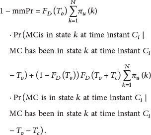$F_{D} (t)$ , of the upstream end-to-end delay as follows:

\begin{matrix} 1 - m m P r = F_{D} (T_{o}) \sum_{k = 1}^{N} π_{u} (k) \cdot P r (MC  is  in  state k at  time  instant C_{i} ∣ MC  has  been  in  state k at  time  instant C_{i} - T_{o}) + (1 - F_{D} (T_{o})) F_{D} (T_{o} + T_{c}) \sum_{k = 1}^{N} π_{u} (k) \cdot P r (MC  is  in  state k at  time  instant C_{i} ∣ MC  has  been  in  state k at  time  instant C_{i} - T_{o} - T_{c}) . \end{matrix}

(3)

Thereby,

π_{u}

is the steady state probability vector of the Markov model at the moment just before the updates are sent by the sensors. The first term considers the case that the last update message reaches the controller in time before the start of the control computation; the second term considers the case that the last update does not arrive in time, but the previous update does. The above equation yields an upper bound for the mismatch probability as other cases; n last updates do not arrive in time but

(n + 1) t h

does, for

n \geq 2

are not considered in detail, but all these cases are mapped into a mismatch (hence, the resulting upper bound).

When implementing (3), the state $π_{u} (k)$ and the detailed composition of the conditional probabilities (which basically are the diagonal elements of products of the form $P^{i} \cdot C^{j} \cdot P^{k}$ ) depend on the cycle duration, the offset $T_{o}$ , and the computation and downstream delay. Therefore, the Markov transition probabilities in the sums can be obtained from adequate products of the matrices P and C; we skip the technical details here.

4.4. Offset Optimization

The above analytic model can be used to obtain optimal offset choices by simple numeric minimization with respect to $T_{o}$ . Figure 7 shows the result of the analytic mmPr model from the previous section, when applied to the scenario analyzed in Section 3; the corresponding control performance graph is in Figure 5 and showed a minimum around an offset choice of 90 ms. The Markov model with different state-sizes $N = 2, \dots, 12$ is fitted to a trace of sensor 3 that has been obtained from a closed-loop control simulation with ideal network. The analytic mismatch metric calculations show a minimum (marked by a cross) around an offset value of 50 ms (when using $N = 8$ states or less) and this minimum shifts to 37.5 ms for $N = 9, \dots, 12$ states. The shift of the minimum to the left can be intuitively explained as follows: The more states are used in the Markov model, the more the mismatch probability is influenced by small changes in the sensor information, so the mismatch metric becomes more sensitive to information age. With smaller offset, the information at the controller is fresher given that it arrives in time. So, this gain in freshness here seems to overcompensate the effect of late arrival of messages for some range of offsets. As Figure 7 shows, the absolute value of the mismatch metric depends on the number of states in the Markov model; however, the benefit of the model is not the absolute value but that it allows determining an optimal offset.

Figure 7

mmPr of sensor 3 for different number of Markov States.

4.5. Sensor mmPr Simulation Results

Figure 8 shows the mmPr of sensor 3 for different offsets found both via the full cosimulation (solid blue curve) and from the model of the sensor information dynamics (dashed red and green curve). All curves are simulated using the same scenario parameters, as described in Section 3.1. The red curve is found from a Markov chain containing $N = 5$ states, while the green curve contains $N = 4$ states. These are chosen as they are the number of states that match the blue curve most closely, both in mmPr values and in optimal offset.

Figure 8

mmPr of sensor 3 for different offsets: the solid curves show the simulation result together with the 95% confidence interval (dotted); the two dashed curves show the model-based result for Markov models with $N = 4$ and $N = 5$ states.

Note that the simulation of the mmPr also takes a discretized version of the sensor space as basis, that is, $m m P r (ϵ) ≔ P r (| X_{s} (C_{i}) - X_{c} (C_{i}) | > ϵ)$ . A smaller discretization level ϵ would lead to higher mismatch probabilities. The simulation takes the whole value space of all sensor values for all offsets and uses an ϵ which is 1/20 of this range. Note that this does not correspond to a Markov chain with $20$ states, as the Markov chain is fitted to only one simulation run (with an ideal network) and hence the value range is smaller for that fit. It turns out that a Markov chain between $N = 4$ and $N = 5$ states has the similar discretization level as assumed for the simulated mmPr.

The control performance that is analyzed in Figure 5 is, however, influenced by the information quality of all three sensors. Therefore, Figure 9 shows the average mismatch probability, where the average is taken over the simulated and model-based values for all 3 sensors when using the same offset. Note, however, that different sensors with different dynamics and different end-to-end delays could also use different offset values. In this paper, however, we restrict ourselves to the analysis of the case when the same offset is applied to all three sensors. The number of states is the same for each sensor, and these values are chosen because they matched the curve in Figure 8. We see that while the curves still match in terms of optimal offset, there is a distinct difference in the mmPr values that each curve takes. The optimal offset for $N = 4$ and $N = 5$ in Figure 9 is in both cases at 62.5 ms.

Figure 9

Mean mmPr of all sensors for different offsets: the solid curves show the simulation result; the two dashed curves show the model-based result for Markov models with $N = 4$ and $N = 5$ states.

Figure 10 compares the accumulated damage of the wind turbine of the offset chosen from the model and the offset found via heuristic methods. Cases 1 to 5, as described in Table 2, are also shown in Figure 6, case 6 (yellow colour) denotes the offset found via the mean mmPr of all 3 sensors, while, for case 7 (green colour), the offset is found based on the mmPr of sensor 3, in both cases for $N = 5$ . We see that for the mean case the accumulated damage is slightly lower; however, the two cases are still within each other's confidence interval.

Figure 10

Controller performance in terms of accumulated damage of, respectively, the baseline case, the heuristic cases, and the model cases.

5. QoS Parameters of Communication Technologies

We have in the previous section made assumptions regarding the end-to-end delay, which was modelled by a shifted exponential distribution with a mean of 31 ms. However, for different communication technologies in the Access and Sensor Networks, the delays experienced may vary, and also other types of delay distributions as well as correlations between subsequent delay values may occur. In this section we investigate the delays of different communication technologies and afterwards use these delay traces to determine the end-to-end delay in the cosimulations.

The aim of the measurement setup for the Access Network was to mimic the communication pattern generated between the central controller and 30 gateways on the wind farm communication network in order to characterize the network properties in terms of delays and packet losses. For each of the technologies, ICMP ping measurements are performed with 64 bytes of application layer payload in the uplink (i.e., for the sensor measurements) and downlink (i.e., for the control commands) roughly corresponding to an actual size of the messages [18]. In further subsections, details of measurement setups for each of the technologies are given, while Section 5.4 describes the measurement setup for the Sensor Network.

5.1. 2G/3G Measurement Setup

The test-bed setup for conducting cellular 2G/3G measurements is comprised of three Huawei E392 USB modems [19] equipped with SIM cards from Austrian telecom provider YESSS. Three SIM cards connected to the modems are provisioned to allow both GPRS and UMTS transmission access. Furthermore, the equipment is placed indoors, in the same room on the second floor of an eight-floor office building. First, the modems are configured to have access only to a GPRS network. Through each modem, ten ICMP ping connections were executed in parallel with a time interval of 150 ms between the probes; thus, 30 connections in total were running in order to mimic the communication pattern between the gateway and the central controller. Subsequently, the same procedure is repeated for the 3G network by configuring the modems for UMTS transmissions. In both cases, around 4000 measurements are collected from each ICMP ping connection during a week day between 11 am and 12 am. The resulting distribution of the measurements for 2G and 3G, respectively, can be seen in Figures 14 and 11. The distance between the modems and GPRS/UMTS base transceiver stations (BTS) is around 30 m, since the stations are located on top of the same building.

Figure 11

PDF of the 3G RTT measurement results.

5.2. PLC Measurement Setup

Powerline communication technology is evaluated with narrow-band Devolo G3-PLC 500 k PLC modems [20], having a total throughput capacity of 240 kbps. Five such PLC modems are connected via power lines of approximately 1 meter length in total, which is much shorter than an actual implementation where they would potentially be hundreds of meters long, making this a best case scenario. In an initial test, three parallel ICMP ping connections are ran from three different PLC modems (9 connections on the PLC network), with 150 ms time interval. It is shown later that, for nine connections running over a PLC network, the network performance is impractical for the wind farm controller due to high delays and packet losses even in this best case setup with short distances.

5.3. WiFi Measurement Setup

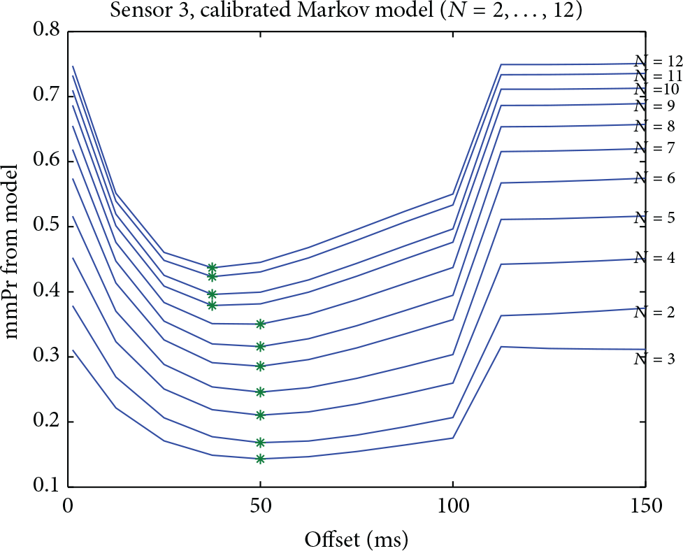
WiFi technologies are tested using two commercially available embedded boards “ALIX 3D2” [21], which allow different IEEE 802.11 hardware modules to be added onto the system. For this study, we connected the 802.11 g (2.4 GHz band) modules of type CM9-GP Wistron [22] onto the boards. The WiFi points are placed indoors within the same room, on the distance of approximately 3 meters, line-of-sight, which again is shorter than an actual implementation, making this a best case setup. In the vicinity of the WiFi points, 23 other networks were scanned; 16 of them were running on 2.4 GHz band, thus adding some interference to the signal; the transmission power is set to 15 dBm. Over such WiFi link, 30 parallel ICMP ping connections were executed during a work day between 3 pm and 5 pm, with the same interval as before. The resulting delay distribution observed on the link is shown in Figure 12.

Figure 12

PDF of the WLAN RTT measurement results.

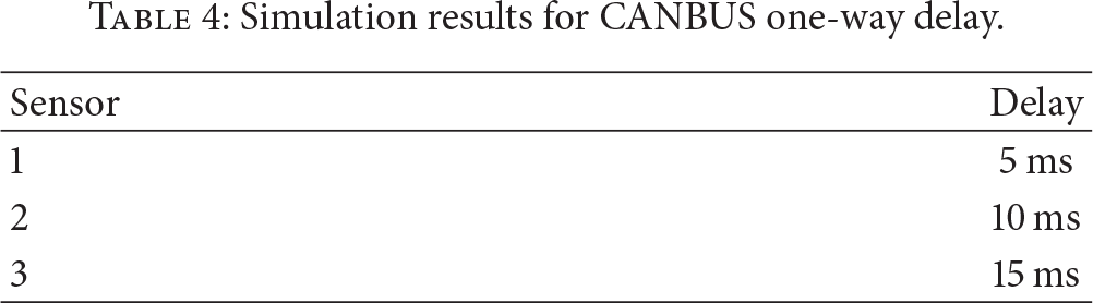
5.4. CANBUS Simulation Setup

The CANBUS is set up with 3 sensors and 1 gateway connected to the CANBUS, with the gateway having the highest priority, then sensor 1 followed by sensors 2 and 3, respectively. The CANBUS is transmitting with 500 kbps and 0% packet loss on the connection. There are no other modules connected to the BUS to generate cross-traffic. Each sensor is set to transmit at the same offset $T_{o}$ once each control period (every 150 ms). The CANBUS is implemented in OMNeT++ and simulated.

5.5. Delay Results

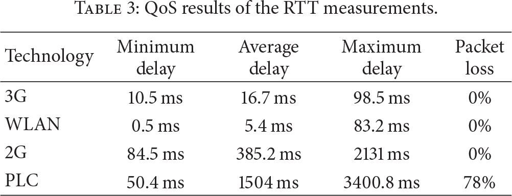
As explained previously, the delays measured on the different technologies, and thus the results shown in this section, are all RTT delays and can be seen in Figures 11–14 and in Table 3. The results in Table 4 are, however, one-way delays. As can be seen in Figure 11, there are two peaks to the 3G measurements. The first peak is at roughly 15 ms, and the other, smaller, peak is at 20–22 ms. We have outliers of the data as high as 98.5 ms, which can be caused by spikes in traffic on the base station. In contrast to the measured delay distribution for 3G, the delays of WLAN in Figure 12 by shape appear like an exponential distribution with a small shift. Similar results, delay-wise, can be seen in [5], however, with a slight different distribution, most likely to be attributed to cross-traffic.

Table 3

QoS results of the RTT measurements.

Technology	Minimum delay	Average delay	Maximum delay	Packet loss
3G	10.5 ms	16.7 ms	98.5 ms	0%
WLAN	0.5 ms	5.4 ms	83.2 ms	0%
2G	84.5 ms	385.2 ms	2131 ms	0%
PLC	50.4 ms	1504 ms	3400.8 ms	78%

Table 4

Simulation results for CANBUS one-way delay.

Sensor	Delay
1	5 ms
2	10 ms
3	15 ms

Figure 13

Time series of the 2G RTT measurement results.

Figure 14

PDF of the 2G RTT measurement results.

From the 30 2G connections we take the data from a single connection on sim card 2 and plot it as a time series in Figure 13. The measurements of the other connections show the same trend as we see in Figure 13. We see low delays at start of the measurements, which may be caused by not all sim cards and/or connections being set up right away. We see a few spikes in the delays between 0 and up until sample number 4250, which can be caused by spikes in traffic on the base station. After measurement 4250, we start to see a steady increase in delays, most likely caused by increased traffic leading to longer queues on the base station and in the sim cards. For the evaluation later, we only use the samples from 250 to 4250, in order to avoid the large instability period that occurs after. Table 3 and Figure 14 show the distribution of these 4000 samples.

Results from the PLC measurements show that the average delay is several control cycles long, and the packet loss is 78%, even for only 9 parallel connections. This is rather problematic for the controller, as it will lead to instability and the controller being unable to generate set-points. For this reason, these results are not used further in this paper, as it is clear from the statistics that the solution is not feasible. The statistics for all the measurements results can be seen in Table 3.

The delays from the CANBUS simulation show deterministic delays for each sensor, with sensor 1 having the lowest delay as it has the highest priority. Each delay is the one-way delay and there were no packet losses experienced. The delay values are summarized in Table 4.

The results of the measurements are used as a time series in the cosimulation framework in order to determine the delays of individual messages. The measurements we have access to are, as explained above, RTT ping messages, except for the CANBUS delays. The delays we are interested in are, however, one-way delays. Therefore, we assume that the uplink and downlink channel properties are identical and we can thus divide the RTTs by 2 to get one-way delays. This represents an approximation as many technologies differentiate in their handling of uplink and downlink data streams.

6. Wind Farm Control Using Cellular Communication Technologies and CANBUS

In this section we use the delay traces found in Section 5 to create different simulation scenarios. To start, we create scenarios where only the Access Network delays are used, and we simulate this scenario using the traces of the technologies for this network. We then create a combination scenario, where we use both the traces from the 3G measurements, as well as the delays incurred by the CANBUS in the Sensor Network. This scenario, thus, entails both networks, creating a simulation of the entire system. The performance of the controller is described by two metrics: reference tracking and accumulated damage of the wind turbine. Analogous to Section 3, we focus on the second metric, the accumulated damage. The simulations are done using the same framework as described in Section 3, where the end-to-end delays both in uplink from sensor to the central controller and in downlink from the central controller to the local controller are obtained now by the traces from the technology measurements in Section 5.

6.1. Control Performance over Cellular Access Technologies

The accumulated damage for the 3G trace (Figure 15) shows an increase in low offsets when offsets get smaller than ≈40 ms, and a sharp increase at an offset of 100 ms. Both of these increases are expected, as at 100 ms offset the computational delay of the central controller means that the control set-point is not yet received. At low offsets, there is a higher chance that the messages will be delayed past the control point $C_{i}$ , and thus old data will be used. The optimal offset is between 37.5 ms and 100 ms, where no statistically significant differences between those offset choices can be observed.

Figure 15

Accumulated damage of wind turbine based on 3G measurements with 95% confidence intervals.

Figure 16 shows the control performance when using the 2G data that was the basis for the pdf in Figure 14. As 2G delays are generally rather long, on average more than 1 control cycle, the controller will in this case most of the time use sensor measurements which are several control cycles old. Figure 16 shows that in this case the control performance is about twice as bad as in the better 3G cases; furthermore, the detailed choice of the offset within the control period is irrelevant as the sensor measurement will be outdated by the time it arrives at the controller anyway. Therefore, there is no offset optimization beneficial for this 2G case given the short control periods of the central controller.

Figure 16

Accumulated damage of wind turbine based on 2G measurements with 95% confidence intervals.

For comparison to the other technologies, a simulation with an ideal network, meaning a network with 0 ms delays and 0% packet loss, has also been executed. The result of this can be seen in Figure 17. This shows a relatively flat curve until an offset of 100 ms, at which point we again see an increase in accumulated damage, as expected based on previous simulation results. We have not included the figure for accumulated damage for the WLAN technology in this paper, as the results are very similar to the results for the ideal network. The biggest difference was in a small increase at offsets below 50 ms; however, this increase was so slight to be within the 95% confidence interval of the ideal network simulation.

Figure 17

Accumulated damage of wind turbine based on ideal network.

6.2. Combined 3G and CANBUS Scenario

Finally, we compare the analytic model in a scenario that mimics the use of 3G access for connections to the wind turbines and a CAN network for the sensor data access with delays as stated in the previous sections. Figure 18 shows a simulation run where the 3G trace is used, as in Figure 15, and the deterministic delay of the CANBUS is added to the delay between the sensors and the central controller. The figure shows a sharper drop in the accumulated damage than for the pure 3G simulation yet is, otherwise, very similar within the 95% confidence intervals.

Figure 18

Performance of controller under combined 3G traces and CANBUS delays.

In order to analyze the impact of the downstream delay from the central controller to the wind turbine, another simulation run like in Figure 18 has been conducted but now with a deterministic downstream delay with the same mean (8.35 ms). The resulting control performance curve did not show any visual difference and any deviations were minor compared to the confidence intervals. As a conclusion, the deterministic assumption for the downstream delay, as taken for the analytic model, does not change the control behavior in this scenario. We also ran a simulation of the scenario in Figure 18, where the correlation in the UMTS delays used in the upstream (from sensor to controller) was destroyed by scrambling the delay trace. Also, in this case, the control performance did not significantly change. Hence, the assumption of a renewal process for the upstream delays in the analytic model does not have any impact for this scenario.

As the analytic model assumes a shifted exponential delay distribution for the access to the sensor data and a deterministic downstream delay, and since we want to see the differences caused by other model assumptions, we, however, do not use the trace of the 3G delay measurements but rather fit a shifted exponential distribution to the parameters of Table 3; and analogously, we use also in the simulation a deterministic downstream delay with the parameter matching the mean 3G delay. We call this the exponential approximation of the combined 3G and CANBUS scenario.

Figure 19 shows the accumulated damage resulting from such a simulation run with varying offset $T_{o}$ for the sensor information access. Figure 19 shows a clear minimum for offsets between approximately 25 ms and 87.5 ms, taking the 95% confidence intervals (marked dashed) into account. Figures 18 and 19 show very similar performance, the main difference being the accumulated damage at $T_{o} = 37.5$ ms, with Figure 19 having higher accumulated damage, however still within the confidence intervals of each other. The relative flat curves for offset between 50 ms and 87.5 ms are due to the rather low variability of the 3G delays.

Figure 19

Performance of controller using deterministic downstream delay and a shifted exponential fitted to the 3G traces.

Figure 20 now takes the Markov models for sensor 3 (with the same calibration as earlier, as this calibration is independent of network delays) of sizes $N = 2, \dots, 12$ and applies the mmPr calculations to these Markov models. The curves show minima around 40 ms while, for small N, they are rather flat in the interval $40 m s \leq T_{o} \leq 90 m s$ .

Figure 20

mmPr over changing offsets for sensor 3 in the exponential approximation of the combined 3G and CANBUS scenario.

Control performance of the system simulated in Figure 19 is, however, influenced by all 3 sensors. In the CAN setting, the 3 sensors have different CAN delays. The analytic model can also be used to calculate mismatch probabilities for each of these sensors. Figure 21 shows the resulting average over the 3 sensors for the mismatch probability. The curves show the same shape as Figure 19, while the optimal offset remains at around 40 ms. Nevertheless, by comparison of Figures 20 and 21 with the simulated control performance in Figure 19, it becomes clear that the approach to use data quality metrics, here, mismatch probability, has general potential for optimizing control performance in periodic control systems.

Figure 21

Average mmPr of all 3 sensors over changing offsets in the exponential approximation of the combined 3G and CANBUS scenario.

7. Conclusion

In this paper, we investigated the impact of end-to-end communication delays and sensor access scheduling optimization on the performance of a wind turbine controller as part of a Smart Grid use-case. We started by determining in Section 3 that there indeed was an impact of the communication network delays, and that an optimized choice of the offset, defined as the time interval between sensor information update generation and controller computation, can be used to improve controller performance. We found that using a simple heuristic to determine the offset ran the risk of choosing a suboptimal offset, and that determining the optimal offset is not a trivial task. In Section 4, we modelled the sensor information dynamics to use an analytical approach to determining the optimal offset, instead of relying on extensive simulations of the controller and network together. We found that it was possible to use the mmPr metric to determine an offset, and that this chosen offset performed as well as, within a 95% confidence interval, or better than the considered heuristic methods. Lastly, we investigate the impact of imperfect communication on controller performance using different communication technologies in Section 5. The delays found from this analysis were then used to simulate the performance of the wind turbine controller once again, and the analytical models were used to find the mmPr of the sensors. We find that due to the low variability of the 3G data there is a rather large offset range in which to choose the optimal offset. The measurements of WLAN data had even lower variability and would not lead to a narrower offset range. Alternatively, the delays of the 2G data were too long for offset optimization to make sense in the chosen scenario. However, for controllers with longer control periods, the 2G data might be more interesting to make offset optimization for, due to the increased variability of the delays.

Future work will look at the impact of different control period choices: slower network technologies like 2G may still be utilized when running the controller less frequently; however, the trade-off of modifications in the control period given a certain end-to-end delay will need to be analyzed and understood. For the analysis of this paper, we assumed that the exchange of sensor values to the central controller and of set-points to the local controller is executed via a very lean protocol, containing just the actual values and a few bytes of information type. The analysis of the impact of intermediate layers like TCP [8, 23] or protocols that try to achieve real-time bounds and reliability [5] or just improve performance behavior of off-the-shelf shared transmission media [24] for the setting of the wind farm control is interesting for future work.

An assumption made in this paper was perfect clock synchronization between the central controller and the sensors. This may not be the case and could cause the offset $T_{o}$ chosen at the sensors to drift, time-wise. This could be fixed by including time synchronization packets on the network; however, this would increase traffic and could increase the delays on the communication network.

This work has been done for a specific Smart Grid scenario; however, in future work, it would be interesting to expand to cover other scenarios, for example, a voltage control scenario as in [25].

Footnotes

Competing Interests

The authors declare that they have no competing interests.

Acknowledgments

The authors would like to thank José de Jesús Barradas-Berglind for lending his wind turbine control simulation and allowing us to work with it. This work was partially supported by the Danish Council for Strategic Research (Contract no. 11-116843) within the Programme Sustainable Energy and Environment, under the EDGE (Efficient Distribution of Green Energy) research project and by the SmartC2Net research project, supported by the FP7 framework programme under Grant no. 318023.

References

Mets

Ojea

J. A.

Develder

Combining power and communication network simulation for cost-effective smart grid analysis

IEEE Communications Surveys and Tutorials 2014 16 3 1771 1796

10.1109/SURV.2014.021414.00116

2-s2.0-84906782750

Bhattarai

B. P.

Lévesque

Maier

Bak-Jensen

Pillai

J. R.

Optimizing electric vehicle coordination over a heterogeneous mesh network in a scaled-down smart grid testbed

IEEE Transactions on Smart Grid 2015 6 2 784 794

10.1109/TSG.2014.2384202

2-s2.0-84923935535

Qiu

R. C.

Chen

Guo

Ranganathan

Hou

Zheng

Cognitive radio network for the smart grid: experimental system architecture, control algorithms, security, and microgrid testbed

IEEE Transactions on Smart Grid 2011 2 4 724 740

10.1109/tsg.2011.2160101

2-s2.0-82155167655

Georgievski

Degeler

Pagani

G. A.

Nguyen

T. A.

Lazovik

Aiello

Optimizing energy costs for offices connected to the smart grid

IEEE Transactions on Smart Grid 2012 3 4 2273 2285

10.1109/TSG.2012.2218666

2-s2.0-84872054209

Malinowsky

Grønbæk

Schwefel

H. P.

Ceccarelli

Bondavalli

Nett

Timed broadcast via off-the-shelf WLAN distributed coordination function for safety-critical systems

Proceedings of the 9th European Dependable Computing Conference (EDCC '12)

May 2012

Sibiu, Romania

IEEE

144 155

10.1109/edcc.2012.26

2-s2.0-84864204677

Siemens Siemens AG, 2015, http://www.industry.siemens.com/verticals/global/en/wind-turbine/communication/pages/default.aspx

Contemporary Control Systems Managed Ethernet Switches Ensure Reliable Communications for a Wind Farm in Inner Mongolia 2010 http://www.ccontrols.com/enews/1210story2.htm

Madsen

J. T.

Le Fevre Kristensen

Olsen

R. L.

Schwefel

H.-P.

Totu

L. C.

Utilizing network QoS for dependability of adaptive smart grid control

Proceedings of the IEEE International Energy Conference (ENERGYCON '14)

May 2014

Cavtat, Croatia

859 866

10.1109/energycon.2014.6850526

2-s2.0-84904965853

Brade

Zug

Kaiser

Validity-based failure algebra for distributed sensor systems

Proceedings of the IEEE 32nd International Symposium on Reliable Distributed Systems (SRDS '13)

October 2013

Braga, Portugal

143 152

10.1109/srds.2013.23

2-s2.0-84891549912

10.

Bøgsted

Olsen

R. L.

Schwefel

H.-P.

Probabilistic models for access strategies to dynamic information elements

Performance Evaluation 2010 67 1 43 60

10.1016/j.peva.2009.08.015

2-s2.0-70350568164

11.

Shawky

Olsen

R. L.

Pedersen

Schwefel

H.-P.

Network aware dynamic context subscription management

Computer Networks 2014 58 239 253

10.1016/j.comnet.2013.10.006

12.

Nielsen

J. J.

Olsen

R. L.

Madsen

T. K.

Uguen

Schwefel

H.-P.

Location-quality-aware policy optimisation for relay selection in mobile networks

Wireless Networks 2016 22 2 599 618

10.1007/s11276-015-0986-0

2-s2.0-84930884267

13.

Madsen

J. T.

de Jesus Barradas-Berglind

Madsen

T. K.

Schwefel

H. P.

On the impact of information access delays on remote control of a wind turbine

Proceedings of the IEEE Eindhoven PowerTech

June-July 2015

Eindhoven, Netherlands

1 6

10.1109/PTC.2015.7232741

14.

Madsen

J. T.

Findrik

Drenjanac

Schwefel

Investigating wind farm control over different communication network technologies

DACH Energie Informatics 2015

Berlin, Germany

Springer

129 140

10.1007/978-3-319-25876-8_11

15.

Madsen

J. T.

Findrik

Madsen

T. K.

Schwefel

H.-P.

Scheduling data collection for remote control of wind turbines

Proceedings of the IEEE International Energy Conference (ENERGYCON '16)

April 2016

Leuven, Belgium

16.

de Jesus Barradas-Berglind

Wisniewski

Soltani

Fatigue damage estimation and data-based control for wind turbines

IET Control Theory & Applications 2015 9 7 1042 1050

10.1049/iet-cta.2014.0730

2-s2.0-84929493598

17.

Hansen

K. S.

Database of wind characteristics

March 2015, http://www.winddata.com

18.

Ahmed

M. A.

Kim

Y.-C.

Communication network architectures for smart-wind power farms

Energies 2014 7 6 3900 3921

10.3390/en7063900

2-s2.0-84903700645

19.

4GLTEmall Huawei E392 4G LTE FDD TDD multi-mode data card, June 2015, http://www.4gltemall.com/huawei-e392-4g-lte-multi-mode-data-card.html

20.

Devolo Devolo g3-plc modem 500k, June 2015, http://www.devolo.com/at/SmartGrid/Produkte/devolo-G3-PLCModem-500k

21.

PC Engine alix3d2, June 2015, http://www.pcengines.ch/alix3d2.htm

22.

Mini-Box

Wistron cm9-gp minipci card

June 2015, http://www.mini-box.com/Wistron-CM9-GP-Atheros-miniPCI

23.

Findrik

Pedersen

Sloth

Hasenleithner

Schwefel

H.-P.

Test-bed assessment of communication technologies for a powerbalancing controller

Proceedings of the IEEE International Energy Conference (EnergyCon '16)

April 2016

Leuven, Belgium

24.

Hinterhofer

Schwefel

H.-P.

Tomic

RD2: resilient dynamic desynchronization for TDMA over lossy networks

Proceedings of the IEEE 31st Symposium on Reliable Distributed Systems (SRDS '12)

October 2012

Irvine, Calif, USA

IEEE

231 236

10.1109/srds.2012.57

2-s2.0-84874341764

25.

Findrik

le Fevre Kristensen

Hinterhofer

Olsen

R. L.

Schwefel

H.-P.

Information-quality based LV-grid-monitoring framework and its application to power-quality control

Ad-Hoc, Mobile, and Wireless Networks: 14th International Conference, ADHOC-NOW 2015, Athens, Greece, June 29–July 1, 2015, Proceedings 2015 9143

Berlin, Germany

Springer

317 329 Lecture Notes in Computer Science

10.1007/978-3-319-19662-6_22

Optimizing Data Access for Wind Farm Control over Hierarchical Communication Networks

Abstract

1. Introduction

2. System Overview

2.1. Communication Network Architecture

2.2. Controller Design

3. Controller Performance under Communication Network

3.1. Scenario Parameters

3.2. Performance Results of Heuristic Cases

4. Model-Based Offset Optimization

4.1. Information Quality Metric

4.2. Markov Model of the Controlled System

4.3. Analytic Model for the Mismatch Probability

4.4. Offset Optimization

4.5. Sensor mmPr Simulation Results

5. QoS Parameters of Communication Technologies

5.1. 2G/3G Measurement Setup

5.2. PLC Measurement Setup

5.3. WiFi Measurement Setup

5.4. CANBUS Simulation Setup

5.5. Delay Results

6. Wind Farm Control Using Cellular Communication Technologies and CANBUS

6.1. Control Performance over Cellular Access Technologies

6.2. Combined 3G and CANBUS Scenario

7. Conclusion

Footnotes

Competing Interests

Acknowledgments

References