
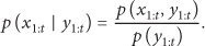
Abstract
We investigate the problem of tracking mobile targets in wireless sensor networks. We propose an advanced auxiliary delayed-weight particle filter algorithm (ADWPF). We make a deep study on the evolvement of particles and formally define the tree-like structure relationship among particles based on observations. Most importantly, we add some auxiliary particles to these structures formed by sampled particles in order to obtain more efficient structures. Based on the newly tree-like structures formed by auxiliary particles and sampled particles, we design a well efficient delayed-weight algorithm with linear computation cost. Experiment results demonstrate that our algorithm can greatly improve the tracking accuracy of a mobile target, compared with bootstrap filter, auxiliary particle filter, and another delayed-weight particle filter.
1. Introduction
In recent years, tracking mobile targets in wireless sensor networks has attracted more and more attention of the researchers in academia and industry [1–3]. This technology has fairly good application prospects in indoor environments, such as shopping mall and underground parking.
Obviously, particle filter is one of the most important technologies for tracking mobile targets in wireless senor networks. Many researchers in [4–6] have utilized particle filter to track the mobile targets in wireless sensor networks. Obviously, the performance of particle filter algorithm has a great impact on the tracking accuracy. So it is very meaningful and important to design an efficient particle filter algorithm. This is also the motivation of our research.
In our paper, we propose an auxiliary delayed-weight particle filter algorithm (ADWPF). Our main contributions are as follows: We make a deep study on the evolvement of particles and give the formal definition of the tree-like structure relationship among particles based on observations. We add some auxiliary particles to the well-defined tree-like structures formed by sampled particles in order to get more efficient structures. These auxiliary particles can greatly help to improve tracking accuracy. Based on the newly tree-like structures formed by auxiliary particles and sampled particles, we design a well efficient delayed-weight algorithm with linear computation cost, whose time complexity is
The remainder of this paper is organized as follows. Section 2 reviews the related work in the area of particle filter and delayed-state filtering. In Section 3, we briefly overview the particle filter and describe the key technologies applied in our algorithm. In Section 4, we describe the deduction and the framework of our algorithm. Section 5 presents simulation results for a self-navigation problem in wireless sensor networks. Section 6 makes the conclusion.
2. Related Work
The particle filter algorithm has been widely used to infer the latent states of stochastic dynamic systems in [7]. It uses the sequential nature of stochastic dynamic systems to generate sequentially weighted Monte Carlo samples, and these samples are used to infer the latent states. For example, in the problem of self-navigation for a mobile target in wireless sensor networks, the position of the mobile target at each time step is the latent state to be inferred.
The bootstrap filter in [8] was the first successful application of the particle filter to the field of nonlinear filtering. It utilizes transition density function as the importance distribution to generate Monte Carlo samples of latent states. Then it assigns the weight of each sample based on the likelihood of the measurement. However, outliers that occurred in the measurement data will decrease the performance of the bootstrap filter as pointed in [8].
In order to increase the robustness of the sampling procedure and obtain approximate samples from the optimal importance distribution, which could minimize the variance of importance weights, [9] introduced the auxiliary particle filter. This algorithm can efficiently reduce the variance of samples' weights.
Reference [10] pointed out that the “future” measurement information can be utilized to improve the estimation accuracy of current system state and mitigate degeneracy of the importance weights over time. So the approximations of the “earlier” marginal distributions of latent states will not collapse as time increases. Reference [10] introduced some delayed-sample methods, such as the Exact Lookahead Sampling method in [11] and the Block Sampling method in [12]. The key technology of these methods is to design an efficient importance distribution, which utilizes “future” information to generate weighted samples of the current states.
In fact, the delayed-sample algorithms which utilize “future” information to generate samples of current states are very similar to the smoothing algorithms which utilize current received measurement information to smooth the marginal filtering distributions of historical hidden states. Reference [10] also pointed that these two methods have very close relationship. Traditional smoothing algorithms mainly include the forward filtering-backward smoothing algorithm and the two-filter smoothing algorithm in [13]. The former is relying on the particle implementation of the forward filtering-backward smoothing formula to reweight the historical filtered samples, and the latter is based on the particle implementation of the two-filter smoothing formula to regenerate weighted samples for the historical hidden states. These two methods have time complexity
3. Particle Filter Algorithm
3.1. System Description
Suppose that the dynamic system [14] is given by the following state and measurement equations:


3.2. Particle Filter
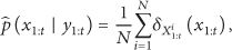
The aim of particle filter is to get the sequential Monte Carlo samples
Step 1 (Initialization). At time where Step 2 (Filtering). At time where
The time complexity is
3.3. Delay Strategy
The key idea of this strategy is that the dynamic system offers more and more information of the latent states as time increases. In order to formalize this fact, assume that the measurement information available at time
Proposition 1.
When the Monte Carlo sample size N is sufficiently large,
For the proof one can refer to [10].
Based on the statement of this proposition, we can design an algorithm that utilizes more and more information to improve the inference about the latent state in a specific time. This lays down the fundament of our work.
There are mainly two methods to implement the idea of Proposition 1 [10]. The first method is the delayed-sample method. It designed an importance distribution, which utilizes measurement information after time t to regenerate weighted samples of state at time t, for example, auxiliary particle filter. The second method is the delayed-weight method, which utilized information after time t to reweight samples
3.4. Relation between Delayed-Sample Method and Delayed-Weight Method
3.4.1. The Problem of Delayed-Sample Method
We know that the most important technology in particle filter is to choose an efficient importance distribution. The optimal importance distribution of the delayed-sample method has the following form [10]:

This optimal importance distribution can generate more effective samples than standard particle filter method, which is based on the one-at-a-time sampling strategy. For continuous state space, it is very hard to adopt this method, since it is not easy to get the explicit form of (6).
3.4.2. Delayed-Weight Method Is a Better Choice
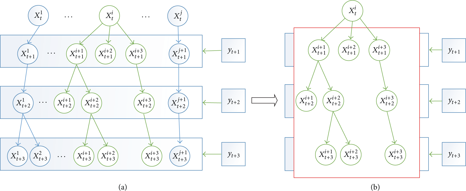
In order to solve the problem of the delayed-sample method, we can discretize the continuous state space using sampled particles, which is the core idea of the delayed-weight method. Figure 1 illustrates the evolvement of particles in the standard particle filter method at time t.

The evolvement of particles in standard particle filter method at time t.
Assume that we observe measurements

Continuous state space can be discretized by weighted particles.
The main advantage of doing so is that the optimal importance distribution

Therefore, the delayed weight

Obviously, this delayed weight can be calculated by the forward filtering-backward smoothing method. We name this method DWFB in [11, 15].
The main disadvantage of this method in [15] is that, in each iteration, we must make use of all particles at time

Since the number of particles is N at time k, the time complexity of this algorithm is
4. An Auxiliary Delayed-Weight Method
Our method consists of two key technologies: designing a backward smoothing procedure and adding auxiliary particles.
4.1. A Backward Smoothing Procedure
Definition 2.
If one particle
Observing the evolvement of particles in Figure 1, some particles have more than one child, while some have no child. Particularly, we observe that a particle and its child/grandchild form a tree-like structure, which is straightforward in Figure 2.
Definition 3.
The tree that consists of particle X and its children/grandchildren is called a generation tree, denoted by
As illustrated in Figure 3, the particles denoted by green circles construct the generation tree

The particles denoted by green circles form
Assumption 4.
If the particle
The main advantage of doing so is that we only need to make use of children/grandchildren of

We only need to use children/grandchildren of
Observing the structure of

Definition 5.
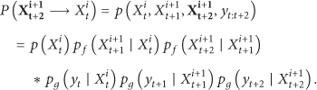
One calls the joint probability function representing the parent-child relation between leaf node
Therefore
More importantly, each backward smoothing term can be decomposed as the product of transition probability functions and likelihood functions; for example, the backward smoothing term
Other backward smoothing terms can be decomposed in the same way. Moreover, from (13), we can see that it is very straightforward to use an iterate method to calculate each backward smoothing term, which is the core idea of our backward smoothing algorithm. Procedure 1 gives the backward smoothing (BS) process from one leaf node to the root node.
( ( ( // the data structure of ( //operation ( ( end (
Obviously, the time complexity of Procedure 1 is

The backward smoothing procedure of Procedure 1. The calculation of each backward smoothing term is iterated from one leaf node to the root node.
4.2. Adding Auxiliary Particles
Experiment results demonstrate that it is not enough to use particles in

Add auxiliary particles to
Definition 6.
One calls the modified generation tree to which auxiliary particles have been added the auxiliary generation tree, denoted by
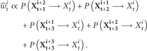
In Figure 6, we also call these newly added auxiliary particles, like
Definition 7.
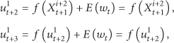
The state of auxiliary particle is defined as the expectation of transition probability function; that is, the auxiliary particles
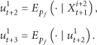
Furthermore, according to the definition of transition probability function (1), we have
According to


Absolutely, each backward smoothing term in (17) can be calculated by Procedure 1.
The main advantage of adding auxiliary particles to the generation tree is that they can greatly improve the filtering accuracy, which is verified in our experiments.
Procedure 2 gives the process of constructing an auxiliary generation tree (CAGF).
Let ( ( ( ( ( ( ( end end ( ( ( ( //add auxiliary particles ( ( ( ( end end end end (
Lemma 8.
The number of leaf nodes in
Proof.
According to step (13) in Procedure 2, only one child is added to every leaf node. So the number of leaf nodes will not increase.
Lemma 9.
Let
The proof is obvious.
4.3. Algorithm Framework
In this section, we first give the framework of our algorithm, and then we analyze its time complexity.
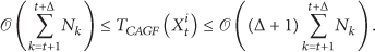
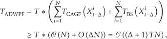
Theorem 10.
The time complexity
Proof.
Obviously, the time cost of Algorithm 3 mainly consists of steps (4) and (6). Let
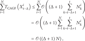

Let
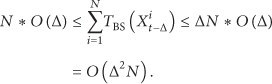
So for the time complexity

Meanwhile,
Assume N is the number of particles, t is current time index, count is the number of simulation steps, ( ( ( ( ( ( ( end end end end The inference result of system state
Let N is the number of particles, t is current time index, and Generate samples end ( ( //Procedure 2. ( ( //Procedure 1. ( ( ( end end end
5. Simulation and Results
To verify the performance of our algorithm ADWPF, we consider a wireless sensor network with 70 anchor sensors

5.1. Linear Motion Model
The state of the mobile sensor evolves according to [16, 17]:

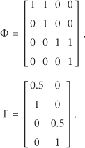
The initial state of the mobile sensor is

Table 1 compares the average MSE for bootstrap particle filter, auxiliary particle filter, DWFB, and our method ADWPF in linear motion model.
Average MSE for bootstrap particle filter, auxiliary particle filter, DWFB, and our method ADWPF in linear motion model.

5.2. Gaussian-Markov Motion Model
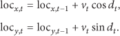
In this test, the target node is moving according to the Gaussian-Markov motion model [18]. In this model, we can use one tuning parameter to vary the degree of randomness of the movement, and the target node will not move out of the deployment area [19]. The speed 
We set
Average MSE for bootstrap particle filter, auxiliary particle filter, DWFB, and our method ADWPF in Gaussian-Markov motion model.

As illustrated in Tables 1 and 2, with N fixed, the MSE values of our method ADWPF with different Δ are all smaller than those of bootstrap particle filter and auxiliary particle filter. Furthermore, with N and Δ fixed, the MSE value of ADWPF is smaller than that of DWFB. Tables 3 and 4 compare the total time cost of bootstrap particle filter, auxiliary particle filter, DWFB, and our method ADWPF in linear motion model (
Total time (sec.) cost of bootstrap particle filter, auxiliary particle filter, DWFB, and our method ADWPF in linear motion model (

Total time (sec.) cost of bootstrap particle filter, auxiliary particle filter, DWFB, and our method ADWPF in Gaussian-Markov motion model (

6. Conclusion
Particle filter is a very important technology for tracking mobile targets in wireless sensor networks. In order to improve the tracking accuracy of the mobile node, we propose an advanced auxiliary delay-weight particle filter algorithm. By adding some auxiliary particles to the generation trees formed by sampled particles, our algorithm ADWPF can efficiently utilize measurement information after time t to reweight Monte Carlo samples
Footnotes
Competing Interests
The authors declare that there are no competing interests regarding publication of this paper.
Acknowledgments
This work has been supported by Hangzhou Key Laboratory for IoT Technology & Application.