Sage Journals: Discover world-class research

Abstract

As the technology of the Internet of Things (IoT) becomes more widely used in large-scale monitoring networks, this paper proposes an optimized obtaining strategy (OFS) for large-scale sensor monitoring networks. First, because of the large-scale features of sensor node network, this paper proposes a large-scale monitoring network area clustering optimization strategy. Second, based on the characteristics of regular changes in the sensed data in large-scale monitoring networks, this paper proposes a strategy for acquiring sensor data based on an adaptive frequency conversion. The OFS optimization strategy can prolong network lifetime, reduce the transmission bandwidth resources, and reduce average energy consumption of the cluster head and network energy consumption.

1. Introduction

In recent years, especially in the big data age [1], the technology of the Internet of Things and the prospects for building applications on this platform have become research hotspots for governments, academia, and industry. A wireless sensor network (WSN) [2], as an important technical aspect of the Internet of Things, can monitor, sense, and sample a wide range of information types from the environment or from monitored objects. A WSN can also process this information in real time [3]. Therefore, WSNs are widely used in large-scale network monitoring. With the development of wireless communication, sensor technology, and embedded computing technology [4], there is an urgent need for applications involving large-scale wireless sensor networks in various fields including the military, intelligent transportation, environmental monitoring, earthquake monitoring, weather disasters, and modern agriculture [1]. However, in these large-scale complex environments [5], wireless monitoring networks pose a series of new problems as follows: the areas that need to be monitored are too large, the number of sensors required is too great, the time overhead of the sensor nodes and the required bandwidth resources and energy consumption of signal transmission are too high. Because monitoring nodes are limited in computing power and storage space, obtaining high-quality sensor data samples and optimizing transmissions to ameliorate the problem of energy consumption [2] and improve the network life cycle have been the core research problems facing the field of large-scale monitoring networks [4, 6].

After analysing the existing research results, this paper proposes an optimized obtaining strategy (OFS) to address the issues facing large-scale monitoring sensor data in the Internet of Things. This strategy can effectively improve the overall operating efficiency of the monitoring network, balance energy consumption, and prolong the network life cycle.

The rest of this paper is organized as follows: Section 2 discusses an optimization strategy that is relevant for both current domestic and international wireless sensor monitoring networks. Section 3 deals with large-scale sensor networks. Because the number of nodes is large and their distribution is uneven, this paper proposes a type of large-scale wireless sensor network area clustering optimization strategy in which a large-scale monitoring network is divided into smaller areas to balance the distribution of cluster heads. It adopts uneven clustering in parallel to alleviate the problem of energy holes [7] in a given area. Section 4 discusses monitoring network data acquisition strategy based on adaptive frequency conversion. This strategy optimizes sensor data sampling using a linear regression model and offers a model compensation mechanism. Section 5 analyses the effectiveness of the proposed optimization strategy through experiments and data comparisons. Finally, the last section provides conclusions.

2. Related Work

Numerous domestic and foreign experts and scholars have carried out in-depth studies aimed at the existing problems of large-scale sensor monitoring networks for the Internet of Things. Younis and other experts proposed the hybrid clustering protocol HEED [8], which first selects preliminary cluster heads based on the residual energy of nodes and then selects a final cluster head based on the results of a competition to determine the clusters' internal communication costs. The communication overhead of this protocol is significant because it needs to carry out multiple message iterations within the cluster radius. A solution was proposed by [5, 9, 10] to resolve energy hole problems by using uneven clustering. However, this solution uses a heterogeneous network [2] in which the cluster head is the super node, and it calculates the deployment location of the node in advance, so there are no dynamically constructed clusters. Researchers in [9, 11] proposed the EECS clustering scheme, which constructs uneven clustering to balance the load by considering the distance between the candidate cluster head and the sink node, but, in this scheme, residual energy exists only in the local comparison node. It does not coordinate node energy consumption overall, and intercluster communication adopts single-hop communication, which limits the scalability of the algorithm and makes it unsuitable for large-scale networks. In [8, 12], the uneven clustering ant colony-based AC-EBUC routing algorithm inherits the advantages of the uneven clustering structure. On this basis, in combination with the ant colony algorithm, it introduces the link reliability parameter and can search multiple paths in real time, but this strategy can easily encounter local optimization problems. A hierarchy of chained network topology was proposed by [13, 14]. This strategy can add extra cluster head nodes to solve energy hole problems based on certain rules, and it significantly prolongs network survival time; however, because of cost, transmission distance time delays, and so on, this strategy is not feasible in large-scale sensor networks. In [15], a VA-DSC compression algorithm is proposed that adopts Slepian-Wolf [16] coding theory and achieves data independent encoding and joint decoding. The data error rate is small, but it needs to transmit all the data after compression. Consequently, the network energy consumption is still high. The TCDCP algorithm proposed in [17–28] can adaptively adjust the acquisition time based on the error between the data and the predicted value of a linear regression model. However, by enhancing the sampling time interval, the absolute value of the error will also increase. Therefore, this algorithm is not applicable in an actual monitoring environment. The linear regression strategy proposed in [18–31] can accurately measure data, adjust the sampling frequency, and reduce the transmission quantity. However, the algorithm is complex and its requirements are too difficult to achieve for sensor nodes. In addition, this algorithm spends too much time constructing the model. In this scheme, if the cluster head node does not receive data for a long period, the model updating process will result in data loss.

3. Area Clustering Optimization Strategy for Large-Scale Monitoring Networks

Most of the above optimization strategies are relatively complex, they cannot adapt well to large-scale sensor monitoring networks. In networks with large numbers of sensing nodes, the message volume of the entire network can increase abruptly, reducing efficiency. Therefore, OFS first adopts an area clustering optimization strategy for large-scale sensor monitoring networks; it then utilizes distributed processing to monitor network sensor data [22].

3.1. Network Energy Consumption Model

Assume that n sensors are arranged randomly in a monitored area. These sensors periodically monitor the environment to collect data. The sink node is located in the centre of the area, so the network covers the entire monitoring area. If $s_{i}$ denotes the ith sensor node, the collection of nodes is $S = \{s_{i} ∣ 1 \leq i \leq n\}$ . This paper uses the typical wireless energy consumption model, as shown in formula (1). When a node transmits l bits of data to other nodes, the distance is d; the energy consumption is the loss sum of the transmitter circuit and power amplification:

\begin{matrix} E_{Tx} (l, d) = \{\begin{cases} l E_{elec} + l ε_{fs} d^{2}, & d < d_{0} \\ l E_{elec} + l ε_{mp} d^{4}, & d \geq d_{0} . \end{cases} \end{matrix}

(1)

In formula (1), $E_{elec}$ denotes the energy consumption of the transmitter circuit, and the symbols $ε_{fs}$ and $ε_{mp}$ denote the energy needed for power amplification in the two models. When the transmission distance d is less than the threshold $d_{0}$ , power amplification loss adopts the free space model. Energy needed for signal transmission is proportional to the square of distance. Conversely, when the transmission distance d is greater than or equal to the threshold $d_{0}$ , it uses the multipath fading model, and the energy is also proportional to the fourth power of distance. As the receiver, node energy consumption is only the transmitter circuit loss. Similarly, the energy consumption of the node receiving l bit of data is

\begin{matrix} E_{Rx} (l) = l E_{elec} . \end{matrix}

(2)

3.2. Network Partition Strategy

As mentioned above, in the existing strategies, the cluster head selection requires all the nodes in the network to make a global judgement. When the number of nodes is large and they are unevenly distributed, all nodes are involved in the comparison, which reduces the efficiency of the whole system [23]. Therefore, this paper proposes a network partition strategy; Figure 1 shows the network partition topology schematic. Sensor nodes are randomly distributed in the monitoring area. The sink node is located in the centre of the area.

Figure 1

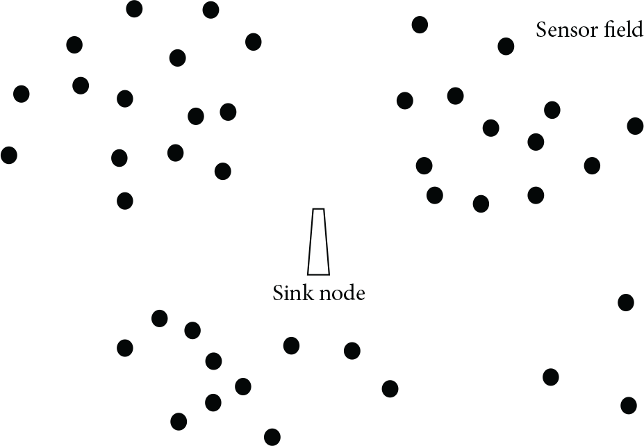
Network partition topology schematic.

As shown in Figure 1, sensor data in the monitoring area are transmitted to the sink node using multihop transmission [22]. This can easily lead to an energy hole around the sink node and then the sensor data cannot be transmitted to the sink node, which seriously affects the network lifetime. Therefore, the OFS strategy adopts the hierarchical clustering algorithm AGNES [19–27]. First, it divides the large-scale network into several subareas, selecting the cluster head and cluster in parallel in each area to boost efficiency. This scheme reduces the energy consumption requirements for all the nodes.

According to formula (1), the energy consumption of data transmission among nodes is closely related to the distance [25]. During network partition, the nodes send their location information to the sink node, which then divides the entire network into several subareas based on distance. Each node can belong to only one area. The distribution of nodes in each subarea is relatively uniform. When this division is complete, the sink node broadcasts relevant information concerning the subarea partitions. Using this broadcast information and its own location, each node can then find the subarea to which it belongs. The divided subarea is fixed over the entire network life cycle to reduce energy consumption from repeated clustering. Meanwhile, to prevent overfitting, the clustering operation needs to set the threshold M, where $M \in (0,1)$ . When the ratio of the number of clustered nodes to the total number of nodes is M, the operation halts clustering. In this way, nodes that are evenly distributed will be divided into one area. The nodes in each area will elect the cluster head via local communication. This solves the problem of misdistribution of the cluster heads and reduces the communication cost. Figure 2 shows a schematic of network partition.

Figure 2

Network partition schematic.

As shown in Figure 2, after clustering, the network in Figure 1 will be divided into 3 subareas of different densities. In the process of data transmission, the sensor nodes in the subarea will transfer their data to the selected cluster head nodes. However, the sensor nodes that are not in the subarea are called outliers. When transferring data, these outlier nodes will select the nearest cluster and either transfer their data to the nearest node in that cluster or transfer the data to the sink node directly. In each area, a distributed uneven clustering strategy is used to alleviate the problem of energy holes based on local competition rules that can improve election efficiency and extend the network life cycle.

3.3. Distributed Area Clustering Strategy

An area clustering strategy collects data periodically. The sink node broadcasts a message to perform network initialization, and each node calculates the distance between itself and the sink node according to the strength of the received messages. Candidate nodes participating in the election maintain a neighbour nodes table and elect a cluster head according to certain rules. The following lists the information available for a neighbour node:

id,

state,

Eres,

dtosk.

In the above, the $i d$ field uniquely identifies one node, and the state field indicates that node's status. The $E r e s$ field represents the remaining energy of the neighbour node, and $d t o s k$ is the distance between that neighbour node and the closest sink node.

Rule 1.

During the election, if a candidate cluster head $s_{i}$ announces that he has won, then all other candidate cluster heads within $s_{i}$ 's competition radius cannot become the cluster head; they must withdraw from the election.

The neighbour nodes set of the candidate cluster head $s_{i}$ contains all the candidate cluster heads that have a competitive relationship with $s_{i}$ given the constraint of Rule 1. During the election, the set of neighbour nodes for candidate cluster head is given by

\begin{matrix} s_{i} \cdot N e b = s_{j}, s_{j} is  the  candidate  cluster  head, d (s_{i}, s_{j}) < \max (s_{i} \cdot R_{comp}, s_{j} \cdot R_{comp}), \end{matrix}

(3)

and the competitive range of every candidate cluster head

R_{comp}

[8] is shown in formula (4), where

d_{m a x}

and

d_{m i n}

represent the maximum and minimum distance between nodes and the sink node, respectively,

d (s_{i}, s k)

represents the distance between

s_{i}

and the sink node, and

R_{comp}^{0}

is the maximum cluster head competitive radius. The value c is a constant between 0 and 1 used to control the range. The competitive range of candidate cluster heads ranges from

(1 - c) R_{comp}^{0}

R_{comp}^{0}

\begin{matrix} s_{i} \cdot R_{comp} = [1 - c \frac{d_{m a x} - d (s_{i}, sk)}{d_{m a x} - d_{m i n}}] R_{comp}^{0} . \end{matrix}

(4)

From formula (4), $R_{comp}$ is a direct ratio function of the distance between this node and the sink node. The distance of the candidate cluster head is reduced as the radius of the competition is reduced. The aim is to create a cluster that is closer to the sink node and with a smaller size, so that cluster head requires less energy to receive transmissions from other members within the cluster. When this occurs, the problem of energy holes diminishes.

After dividing the network, the clustering strategy divides the nodes in each area to control the distribution of cluster heads based on distance. At this point, the nodes in each subarea are relatively concentrated. Using a time broadcasting mechanism, a time threshold t is set up to control the proportion of candidate cluster heads based on the uneven clustering. Then, it is not necessary for each node to become a candidate cluster head. The average residual energy within each candidate cluster head competition radius and the average distance between the nodes and sink node are shown, respectively, in the following formulas:

E_{n} = \frac{\sum_{j = 1}^{m} E_{res}^{j}}{m},

(5)

D_{n} = \frac{\sum_{j = 1}^{m} d (s_{i}, sk)}{m} .

(6)

The value of the time clock is calculated as

\begin{matrix} t = k \times t_{0} \times \frac{E_{n}}{E_{res}^{i}} \times \frac{d (s_{i}, sk)}{D_{n}}, \end{matrix}

(7)

where k is a random number between 0 and 1 to reduce the possibility of time conflicts for broadcast messages,

t_{0}

is defined as the time required for the election of the cluster head,

E_{res}^{i}

is the residual energy of the node

s_{i}

, and

E_{n}

is the average residual energy of node

s_{i}

's neighbour nodes. Formula (7) shows that the candidate nodes closer to the sink node that have more residual energy available for a shorter time have a greater probability of becoming the cluster head.

Within time t, if the candidate cluster head node $s_{i}$ does not receive a successful message from its neighbour nodes, that node will win the election and become the cluster head; otherwise, the election will fail and the node will withdraw from the election process. After election of a cluster head, the ordinary nodes wake up from their sleep state when the cluster head broadcasts a victory message CH_ADV_MSG. The ordinary nodes join the cluster based on the received message by sending the JOIN_CLUSTER_MSG message to the cluster head.

In summary, the OFS optimization strategy performs local uneven division in parallel when the number of sensor nodes is large and the distribution is uneven and dynamically sets the time threshold to control the proportions of cluster head competition, reduce the amount of communication transmission quantity, and balance cluster head energy consumption to effectively improve network efficiency and extend the network life cycle.

4. Adaptive Frequency Conversion Data Acquisition Strategy for Large-Scale Sensor Monitoring Networks

Based on the area clustering described in the previous section that optimizes sensor data acquisition and network transmission energy consumption, this paper proposes an adaptive frequency conversion based sensor network optimization strategy. By analysing the regression model, it can adjust the sampling frequency and update the model dynamically through a mechanism of sensed data compensation and reduced data redundancy.

4.1. Frequency Conversion Sampling Model

A clustered wireless sensor network [20–28] has a chain network topology. Figure 3 shows a schematic diagram of the structure of the sensor network.

Figure 3

Schematic diagram of the structure of the sensor network.

As shown in Figure 3, each sensor node SN can communicate with its next hop node, effectively forwarding data to the cluster head CHN [21] by following a path.

4.1.1. Establishment of Acquisition Model

Through time series analysis, it is found that the sensor message of a single sensor node is similar in continuous sampling; that is, the collected data at the same node over a given a period of time has a high temporal correlation [22–29]. So this study creates a linear regression model that approximately estimates the sensor data [23–30]. Figure 4 shows a schematic diagram of the regression model [30].

Figure 4

Schematic diagram of regression model.

4.1.2. Fitting a Regression Curve

Because of the wireless sensor network nodes' limited computing power and storage space, this paper uses a linear regression model to improve the accuracy of prediction and reduce the complexity of the algorithm [24–31]. Its form is $α^{'} = a + b t$ , where t represents the acquisition time and $α^{'}$ represents the corresponding forecast value of t. A collection of N sensor data, which has been sampled by the nodes in a time sequence, is recorded in the monitoring network:

\begin{matrix} TS = \{(t_{1}, α_{1}), (t_{2}, α_{2}), \dots, (t_{n}, α_{n})\} . \end{matrix}

(8)

TS can be regarded as a linear function based on the sampling time t as the independent variable and the sampled data value a as the dependent variable [25–31]. The linear regression model is fitted according to the least squares method to acquire the least sampling data and minimize the square of the error of the fitting curve:

\begin{matrix} D = \sum_{i = 1}^{n} d_{i}^{2} = \sum_{i = 1}^{n} {[α_{i} - (a + b t_{i})]}^{2} . \end{matrix}

(9)

At the same time, to make the prediction closer to the true values, this paper computes the second-order partial derivative of D to a and b, as follows:

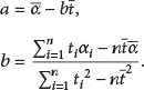
\begin{matrix} a = \bar{α} - b \bar{t}, \\ b = \frac{\sum_{i = 1}^{n} t_{i} α_{i} - n \bar{t} \bar{α}}{\sum_{i = 1}^{n} {t_{i}}^{2} - n {\bar{t}}^{2}} . \end{matrix}

(10)

The values of a and b are the model parameters. The cluster head node utilizes parameters a and b to construct the regression model for a SN node. Then, it can calculate the measurement value of that SN using the model every time the SN would normally take a measurement. This reduces redundant transmissions and the overall energy consumption of the network.

4.2. Adaptive Frequency Conversion Acquisition and Optimization Strategy

Because of the temporal correlation of sensor data [22], sensor data are distributed along the time axis in the prediction model and the optimal strategy can adaptively adjust the acquisition frequency. Figure 5 shows a schematic diagram of adaptive frequency conversion. Set ε as the error range, α as the true value of the acquisition time t, and δ as the difference between the predicted value and the true value; that is, $δ = |α^{'} - α|$ . T is the time interval for the acquisition data.

Figure 5

Schematic diagram of adaptive frequency conversion.

As shown in Figure 5, the actual value of the sensor data will float within the error range, and the initial value of the threshold $β (0 < β < ε)$ is $ε / 2$ . Then, the optimization strategy of a certain period should meet the following rules.

Rule 2.

When $δ \leq β$ , the model can meet the requirements for the time period and can reduce the sampling frequency, and the model can adjust the sampling interval $T = T + Δ T$ ( $Δ T$ is a one-time interval unit). When $T = T_{m a x}$ , the threshold value of β decreases exponentially; $β = 1 / 2 β$ .

Rule 3.

When $β \leq δ \leq ε$ , the actual monitoring value is outside the trend of the forecast model; therefore, the sampling frequency must be increased. In the model, the sampling interval $T = T / 2$ is adjusted adaptively by the exponential form. When $T = T_{m i n}$ , the threshold value of β increases exponentially; $β = 3 / 2 β$ .

The OFS optimization strategy adjusts the sampling frequency adaptively by using real-time monitoring data. The alternative changes of the threshold and the time axis are used to prevent the continuous emergence of a minimum or maximum measurement interval. Network energy consumption is reduced by avoiding data transmission as long as there is a guarantee of measuring accuracy.

4.3. Failure Data Compensation Mechanism

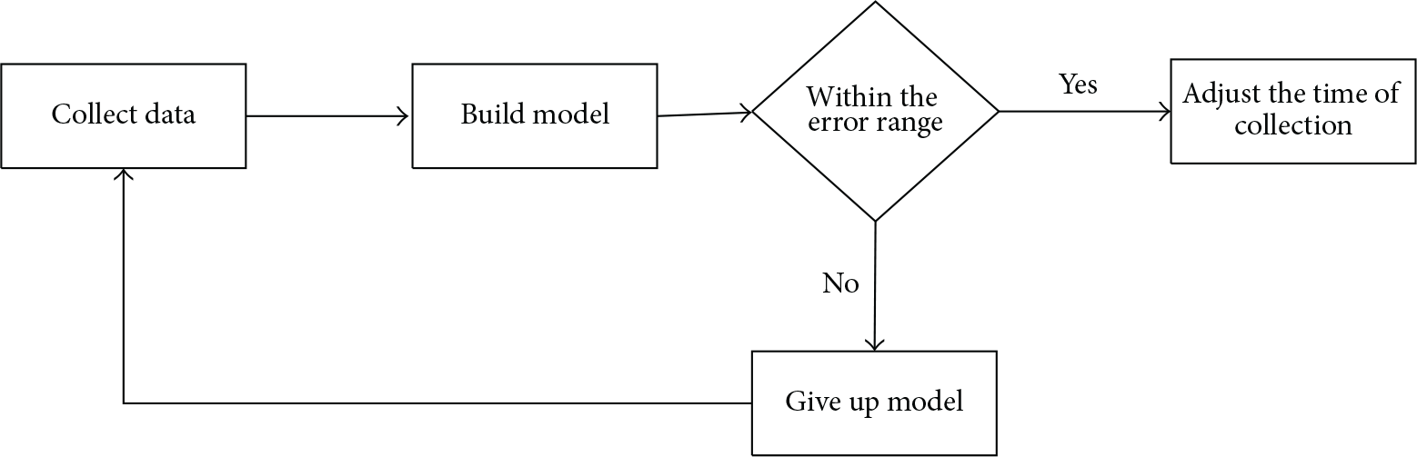
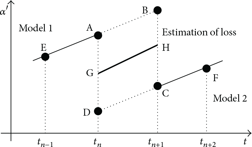
As mentioned earlier, when the regression model fails, the network needs to remeasure and fit a new model, but the inflection point at which the monitoring data causes the model to fail also generates a problem of data loss. Because the inflection point is not predicted and the time of that data inflection point is already in the past by the time the data deviation gets measured, the scheme needs to compensate for this loss of data around the inflection point. Figures 6 and 7 are schematic diagrams that show the failure data compensation mechanism: EA is Model 1 and CF is the updated Model 2. When the old and the new model are replaced, the data will be lost. According to the values of the model parameters, different estimation strategies are used in the compensation mechanism.

Figure 6

Schematic diagram of the failure data compensation mechanism.

Figure 7

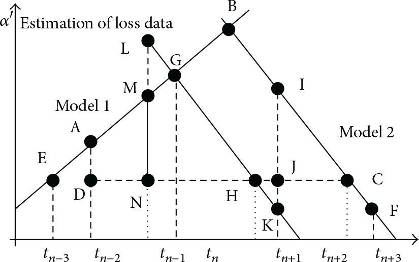
Schematic diagram of the failure data compensation mechanism.

As shown in Figure 6, if Model 1 and Model 2 have the same sign of parameter b, the extension line of Model 1 is AB, and the extension line of Model 2 is CD, then ABCD represents data estimated to be lost. At the same time, the two final measurement points E, A and C, F in Model 2 are the two new starting points selected. These 4 data points will be synthesized into a new linear regression model GH via the least squares principle. In this way, the measurement between Point A and Point C will be deduced at any given moment. At this point, the estimated value must fall in the range of estimation, so the linear regression model of GH is the compensation model for lost data in the time period within $[t_{n}, t_{n + 1}]$ .

As shown in Figure 7, if Model 1 and Model 2 do not have the same sign of parameter b, AB is the extension of Model 1, CB is the extension of Model 2, and the quadrangle ABCD is the estimated range of the missing data. The two final measurement points E, A in Model 1 and C, F in Model 2 are the two new starting points that are selected. These 4 data points are synthesized into a new linear regression model GH via the least squares principle. At this point, the lost data from $[t_{n - 2}, t_{n}]$ and $[t_{n + 1}, t_{n + 3}]$ are beyond the scope of estimation; they need to be calculated again. Using the mean of the method, the compensation model is $α^{'} = 1 / 3 (α_{l}^{'} + α_{h}^{'} + α_{p}^{'})$ . Respectively, $α_{l}^{'}$ , $α_{h}^{'}$ , and $α_{p}^{'}$ represent the intersection of the straight line $α^{'} = 0$ and the model at moment t.

In summary, according to the trend of data in the model, the OFS optimization strategy adaptively adjusts frequency and dynamically updates the model in real time based on the error range. Each SN node will return the respective parameters to the corresponding CHN node. According to the least square method, the CHN node can use these parameters to calculate a regression model for each SN node in the cluster and then obtain the node's sensor data. Subsequently, unless the model fails, the SN node does not need to transmit sensor data to the CHN node, which effectively reduces the quantity of transmissions and reduce network energy consumption.

5. Experiments and Comparison

There are 400 sensor nodes distributed randomly over a 300 m × 200 m area. These sensor nodes monitor changes in temperature during four one-hour time slots distributed throughout a day as follows: 7:00-8:00, 12:00-13:00, 17:00-18:00, and 23:00-24:00. The initial sampling frequency of these sensor nodes is 0.0083 Hz. This experiment tests the feasibility of OFS and gauges its effectiveness using measures of network lifetime, total energy consumption, comparison of node energy balance, error analysis, data acquisition quantity, total quantity of network transmission, and so on. The simulation parameters are shown in Table 1.

Table 1

Simulation parameters.

Parametric description	Value
Node quantity	400
Sensor initial energy $E_{0}$	0.4 J
$E_{e l e c}$	50 nJ/bit
$ε_{f s}$	10 pJ/(b⋅m²)
$ε_{m p}$	0.0013 pJ/(b⋅m²)
EDA	$5$ nJ/(bit⋅signal)
$d_{0}$	87 m
Packet size	4000 bits

5.1. Network Lifetime

Figure 8 shows a comparison of different optimization strategies to maximize network lifetime. Network lifetime can be expressed by the relationship between the numbers of nodes that survive a given number of rounds. At this stage, a cluster head is chosen to join in a round. By capturing the number of rounds from the death of the first node to the death of all nodes, a round can show how well the network balances energy consumption. A greater number of rounds indicate a correspondingly greater efficiency in network energy utilization.

Figure 8

Network lifetime comparisons.

OFS optimizes the residual energy of nodes, the distribution density, and the transmission distance. The network lifetime can be prolonged because weaker nodes can continue to function longer. In Figure 8, compared to LEACH, HEED, and EEUC, OFS prolongs network lifetime by 38%, 15%, and 3.7%, respectively, while also balancing its energy consumption better.

5.2. Comparison of Total Network Energy Consumption

Figure 9 shows the comparison of total network energy consumption for different optimization strategies. To test precisely, when the number of survive nodes drops below 20, we consider the network DEA.

Figure 9

Comparison of total network energy consumption.

The OFS optimization strategy uses a clustering algorithm to divide the network into zones and generates the optimal cluster structure, which distributes cluster head nodes uniformly in the network and reduces energy loss to alleviate energy holes. In Figure 9, when the network has reached 800 rounds, the total network energy of OFS strategy remains 3.456 J, but other strategies have run out of network energy. This result shows that total network energy consumption using the OFS optimization strategy is lower than others.

5.3. Comparison in Consumption of Node Energy Balance

Figure 10 shows the curves of node residual energy variance for different optimization strategies. The energy balance performance can be tested for all these optimization strategies using 10 random rounds. The function of energy variance is shown as (note: the unit is 10⁻³ J)

\begin{matrix} D_{E} (t) = \frac{\sum_{i = 1}^{N} {[E_{i} (t) - {Avg}_{E} (t)]}^{2}}{N} . \end{matrix}

(11)

Figure 10

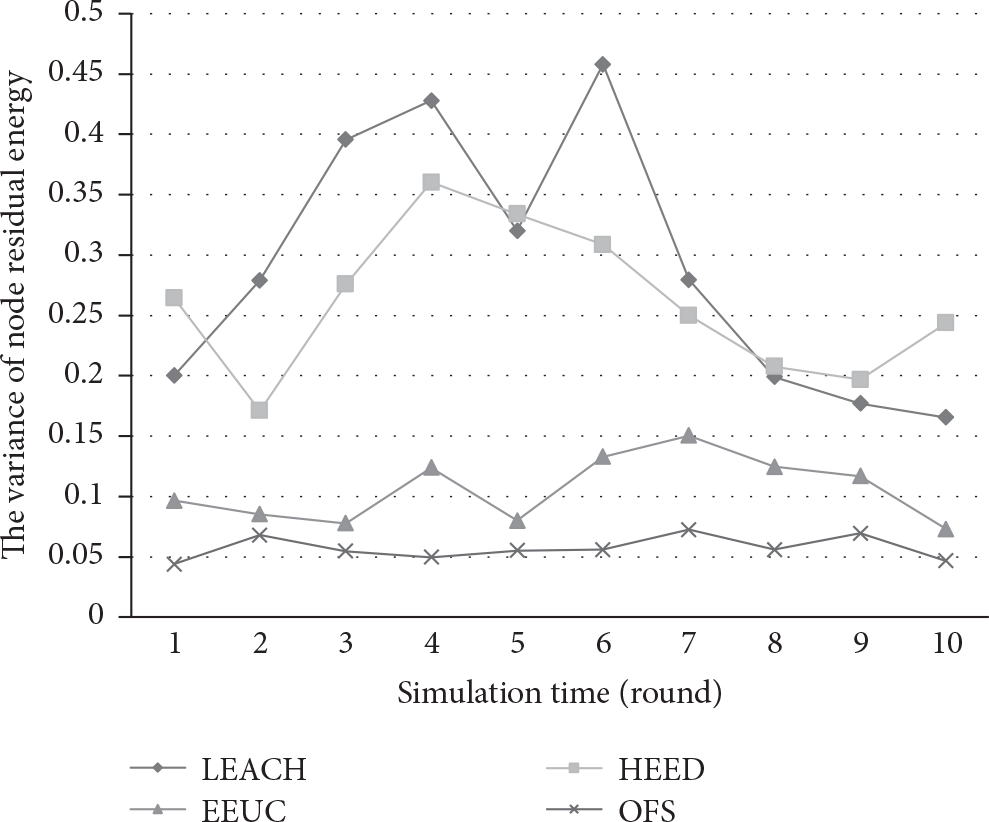
The curves of node residual energy variance.

Compared to other optimization strategies, Figure 10 indicates that the OFS optimization strategy has a more stable curve with fewer fluctuations from node energy variance; therefore, OFS performs better in node energy consumption and energy balance than the compared optimization strategies.

5.4. Error Analysis

Figure 11 shows comparisons of sensor data errors using different optimization strategies. In a fixed time slot, this test randomly selects the absolute value of sensor data from 400 sensors.

Figure 11

Comparisons of sensor data error.

In Figure 11, VA-DSC simply compresses and transfers sensor data. It has the minimum error; the value is 0.07°C. The maximum absolute errors using the OFS linear regression strategies are 0.39°C and 0.43°C, respectively. As the sample interval of TCDCP increases, the absolute error also increases. Absolute error increases to 0.89°C after one hour. The test indicates that OFS achieves slightly lower scores than VA-DSC for error control, meaning that it performs slightly better.

5.5. Data Acquisition Quantity

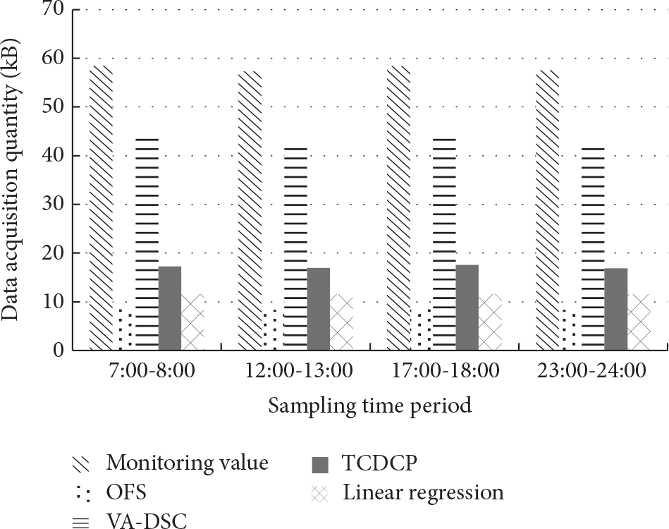
Figure 12 shows a comparison of data acquisition quantity for different optimization strategies. The experiment tested the average value of the data collected by the 400 monitoring nodes over 4 time periods.

Figure 12

Data acquisition quantity.

OFS utilizes the adaptive frequency conversion optimization strategy, which means it can constantly modify the threshold value β and the time interval T according to change trends of sensor data. By doing this, OFS substantially reduces the quantity of data acquisition required. Figure 12 shows that the average data acquisition quantity in OFS is 241.5 KB. The values in the linear regression, TCDCP, and VA-DSC methods are all higher: 264 KB, 283.25 KB, and 357.5 KB, respectively. This result indicates that OFS performs excellently in controlling the quantity of sensor data that must be transmitted.

5.6. Network Transmission Quantity

Figure 13 shows comparisons of network transmission quantity for different optimization strategies. In four time slots, this test selects the average network transmission quantity from 400 sensors.

Figure 13

Network transmission quantity.

Figure 13 shows that OFS needs only two regression parameters when building a model. Therefore, its network transmission quantity is minimum and the average is 8.4 MB. In comparison to the linear regression, TCDCP, and VA-DSC models, OFS reduces network transmission quantity by 27%, 80%, and 85%, respectively. These results show that OFS dramatically reduces the quantity of network transmissions required.

6. Conclusions

With the rapid development of Industry 4.0 and the Internet of Things, large monitoring networks have introduced new problems. The research hotspot for the Internet of Things is still wrestling with these problems. This paper proposes an optimized obtaining strategy (OFS) for acquiring sensor data in large monitored networks connected to the Internet of Things. OFS uses a hierarchical clustering algorithm to divide the network, generating a better clustering structure and reducing network communication overhead. OFS also builds a one-dimensional linear regression model for sensor data that serves to regulate acquisition frequency adaptively, reducing sensor data acquisition and transmission quantity requirements.

The experimental results indicate that OFS can effectively control the energy consumption of sensor nodes to prolong network lifetime. The results of this study provide an effective path for future development of Internet of Things and large-scale monitoring networks.

Footnotes

Competing Interests

The authors declare that they have no competing interests.

Acknowledgments

This work is supported by the National Natural Science Foundation of China (nos. 61502474, 61501105, and 61300233), the Foundation of Science Public Welfare of Liaoning Province in China (no. 2015003003), Major Industrial Project of Science & Technology of Liaoning Province (no. 2012216007), and Doctoral Scientific Research Foundation of Liaoning Province (no. 20141014). This work is also supported by Beilin District 2012 High-Tech Plan, Xi'an, China (no. GX1504) and supported by Xi'an Science and Technology Project (CXY1440 $(6)$ ) and the Specialized Research Fund for the Doctoral Program of Higher Education of China (no. 20136118120010).

References

Sun

Zhang

Bie

Measuring semantic-based structural similarity in multi-relational networks

International Journal of Data Warehousing and Mining 2016 12 1 20 33

10.4018/IJDWM.2016010102

Sun

Yan

Bie

Zhou

Constructing the web of events from raw data in the Web of Things

Mobile Information Systems 2014 10 1 105 125

10.3233/mis-130173

2-s2.0-84892944449

Sun

Jara

A. J.

An extensible and active semantic model of information organizing for the Internet of Things

Personal and Ubiquitous Computing 2014 18 8 1821 1833

10.1007/s00779-014-0786-z

2-s2.0-84921066508

Sun

Bie

Zhang

Semantic relation computing theory and its application

Journal of Network and Computer Applications 2016 59 219 229

10.1016/j.jnca.2014.09.017

Gao

Cai

Gao

Composite event coverage in wireless sensor networks with heterogeneous sensors

Proceedings of the 34rd Annual IEEE International Conference on Computer Communications (INFOCOM ’15)

2015

Sun

Nan

Cluster-based and energy-balanced time synchronization algorithm for wireless sensor networks

Journal of Computer Applications 2014 34 9 2456 2459

10.11772/j.issn.1001-9081.2014.09.2456

Y.-L.

Sun

Y.-F.

Yin

B.-C.

Information sensing and interaction technology in internet of things

Chinese Journal of Computers 2012 35 6 1147 1163

10.3724/sp.j.1016.2012.01147

2-s2.0-84864504617

Younis

Fahmy

HEED: a hybrid, energy-efficient, distributed clustering approach for ad hoc sensor networks

IEEE Transactions on Mobile Computing 2004 3 4 366 379

10.1109/tmc.2004.41

2-s2.0-10944266504

Chen

The energy hole problem of nonuniform node wireless sensor networks

Chinese Journal of Computers 2008 31 2 253 261

10.

Liu

Pei

Survey on node deployment algorithm in wireless sensor networks

Sensor World 2009 15 8 10 14

11.

Zhao

A signal mechanism based energy-aware geographic routing algorithm

Chinese Journal of Electronics 2015 43 5 965 973

12.

Soro

Heinzelman

W. B.

Prolonging the lifetime of wireless sensor networks via unequal clustering

Proceedings of the 19th IEEE International Parallel and Distributed Processing Symposium (IPDPS ’05)

April 2005

Piscataway, NJ, USA

IEEE

10.1109/ipdps.2005.365

2-s2.0-33746310074

13.

Chen

EECS: an energy-efficient clustering scheme in wireless sensor networks

Journal of Frontiers of Computer Science & Technology 2007 3 2-3 535 540

14.

Chen

An uneven cluster-based routing protocol for wireless sensor networks

Chinese Journal of Computers 2007 30 1 27 36

15.

Miao

Chen

Cao

Zhang

Energy balanced uneven clustering algorithm based on ant colony for wireless sensor network

Journal of Computer Applications 2013 33 12 3410 3414

10.3724/sp.j.1087.2013.03410

16.

Dong

R. S.

Z. X.

Guo

Y. C.

T. L.

A Markov game theory-based energy balance routing algorithm

Chinese Journal of Computers 2013 36 7 1500 1508

10.3724/sp.j.1016.2013.01500

MR3136578

2-s2.0-84881621804

17.

Chen

C. W.

Wang

Chain-type wireless sensor network for monitoring long range infrastructures: architecture and protocols

International Journal of Distributed Sensor Networks 2008 4 4 287 314

10.1080/15501320701260261

2-s2.0-54249162967

18.

Hua

Chen

C. W.

Correlated data gathering in wireless sensor networks based on distributed source coding

International Journal of Sensor Networks 2008 4 1-2 13 22

10.1504/IJSNet.2008.019248

2-s2.0-70450250897

19.

Pan

Liu

Low-complexity compression method for hyperspectral images based on distributed source coding

IEEE Geoscience and Remote Sensing Letters 2012 9 2 224 227

10.1109/LGRS.2011.2165271

2-s2.0-84856960306

20.

Wang

Ong

Qike

A. N.

Data compression and optimization algorithm for wireless sensor network based on temporal correlation

Journal of Computer Applications 2013 33 12 3453 3456

10.3724/SP.J.1087.2013.03453

21.

Song

Wang

C.-R.

Linear regression based distributed data gathering optimization strategy for wireless sensor networks

Chinese Journal of Computers 2012 35 3 568 580

10.3724/sp.j.1016.2012.00568

2-s2.0-84860285051

22.

Cheng

Cai

Fang

Drawing dominant dataset from big sensory data in wireless sensor networks

Proceedings of the 34rd Annual IEEE International Conference on Computer Communications (INFOCOM ’15)

April 2015

Hong Kong

IEEE

531 539

10.1109/infocom.2015.7218420

23.

Cai

Cheng

Wang

Approximate aggregation for tracking quantiles and range countings in wireless sensor networks

Theoretical Computer Science 2015 607 381 390

10.1016/j.tcs.2015.07.056

MR3429060

24.

Lian

Naik

Agnew

G. B.

Data capacity improvement of wireless sensor networks using non-uniform sensor distribution

International Journal of Distributed Sensor Networks 2006 2 2 121 145

10.1080/15501320500201276

2-s2.0-34548851055

25.

Sun

Bie

Song

Discovering time-dependent shortest path on traffic graph for drivers towards green driving

Journal of Network and Computer Applications 2016

10.1016/j.jnca.2015.10.018

26.

Chen

Meng

Zhang

Chain-type wireless sensor network node scheduling strategy

Journal of Systems Engineering and Electronics 2014 25 2 203 210

6808324

10.1109/jsee.2014.00024

2-s2.0-84904340767

27.

Guo

Meratnia

Havinga

P. J. M.

Jiang

Zhang

OPS: opportunistic pipeline scheduling in long-strip wireless sensor networks with unreliable links

Wireless Networks 2015 21 5 1669 1682

10.1007/s11276-014-0807-x

2-s2.0-84931274994

28.

C. Z.

Teo

K. L.

Design of discrete Fourier transform modulated filter bank with sharp transition band

IET Signal Processing 2011 5 4 433 440

10.1049/iet-spr.2009.0269

2-s2.0-79960244458

29.

Jiang

Jin

LEAP: localized energy-aware prediction for data collection in wireless sensor networks

Proceedings of the 5th IEEE International Conference on Mobile Ad-Hoc and Sensor Systems (MASS ’08)

October 2008

491 496

10.1109/mahss.2008.4660044

2-s2.0-67650677272

30.

Cheng

Cai

Curve query processing in wireless sensor networks

IEEE Transactions on Vehicular Technology 2015 64 11 5198 5209

10.1109/tvt.2014.2375330

31.

Zhao J.-J. Zhong-Cheng

Zhi-Hua

Hao

I. U.

Bin

I. A. N.

Research of multi-type data fusion in sensor networks

Application Research of Computers 2012 29 8 2811 2816

An Optimized Data Obtaining Strategy for Large-Scale Sensor Monitoring Networks

Abstract

1. Introduction

2. Related Work

3. Area Clustering Optimization Strategy for Large-Scale Monitoring Networks

3.1. Network Energy Consumption Model

3.2. Network Partition Strategy

3.3. Distributed Area Clustering Strategy

Rule 1.

4. Adaptive Frequency Conversion Data Acquisition Strategy for Large-Scale Sensor Monitoring Networks

4.1. Frequency Conversion Sampling Model

4.1.1. Establishment of Acquisition Model

4.1.2. Fitting a Regression Curve

4.2. Adaptive Frequency Conversion Acquisition and Optimization Strategy

Rule 2.

Rule 3.

4.3. Failure Data Compensation Mechanism

5. Experiments and Comparison

5.1. Network Lifetime

5.2. Comparison of Total Network Energy Consumption

5.3. Comparison in Consumption of Node Energy Balance

5.4. Error Analysis

5.5. Data Acquisition Quantity

5.6. Network Transmission Quantity

6. Conclusions

Footnotes

Competing Interests

Acknowledgments

References