Sage Journals: Discover world-class research

Abstract

Network connectivity is a fundamental requirement for intervehicle communication and services in VANETs. The fast movement of the vehicles results in rapid changes in network topology generating dynamic variation in network connectivity, which causes dynamic variation in network connectivity. In this paper, we analyze the evolution of the VANETs connectivity based on the realistic data collected by the GPS devices installed on taxis in Shanghai. The study of the evolution characteristics shows that the number of connected components, the size of the giant component, and the connectivity length time series possess strong temporal correlation and long-range dependence. As a result, the short-range dependent processes such as the exponential, normal, or Poisson distributions cannot capture the statistical distribution characteristics. Moreover, all connectivity parameters cannot be described by unimodal distributions. We also conclude that although the whole topology of the VANETs is broken into a large number of small-sized connected components under small transmission radius, the size of the giant component keeps stable when transmission radius reaches the threshold. These results will be helpful to optimize the RSUs deployment and transmission radius to keep the giant component stable and design more efficient strategies to forward the information in VANETs.

1. Introduction

Vehicular Ad Hoc Networks (VANETs) are considered to be a special application of infrastructureless wireless Mobile Ad Hoc Networks (MANETs) [1]. VANETs have some distinctive characteristics compared with MANETs like road pattern restrictions, large network size, variable network density, highly dynamic topology, infinite energy supply, localization functionality, high computational ability, and so on [2, 3]. Two communication types can be distinguished in VANETs: one is called Vehicle-to-Vehicle (V2V), in which vehicles can exchange information when they are located in the communication range of each other. The other one is called Vehicle-to-Infrastructure (V2I) communications in which vehicles are connected to fixed stations located on the roadsides for information exchange or Internet access. The IEEE 802.11p working group is responsible for the standardization for V2V and V2I communications, while the entire communication protocol stack is being standardized by Wireless Access in Vehicular Environments (WAVE).

Connectivity is one of the most important properties for information dissemination in VANETs, since it represents the available paths for communication. In real applications of VANETs, vehicles move with different speeds and directions; hence, potential connectivity is constantly changing. Thus, network connectivity is a crucial research challenge for achieving VANETs applications.

There are many studies to analyze the connectivity of VANETs. These studies can be broadly divided into three categories. The first category is aimed at developing a model-based theoretical analysis of network connectivity. With exponentially distributed intervehicle distances [4, 5], use a queuing theoretic approach for the connectivity analysis. In [6], the authors have introduced a dynamic connectivity graph and applied it to analyze properties of Poisson network. Zhuang et al. [7] derive the exact expression for the average size of the connected components and their size distribution for one-dimensional VANETs. The authors in [8] use a new approach of using Exponential Random Geometric Graphs (ERGGs) to analyze the dynamic connectivity of VANETs. These theoretical analysis are useful in discussing the critical conditions or the connectivity boundary. But one of the main limitations of abovementioned works related to VANETs connectivity is that these theoretical models still rely on strong assumptions, which are not consistent with real cases. For example, although an exponential distribution is a good approximation for the distribution of intervehicle distance, it is shown that assuming the intervehicle distance distribution is exponential will overestimate the connectivity probability by a significant amount [9].

The second category is a mobility model-based technique for analyzing network connectivity for VANETs. Conceição et al. [10] contrast the connectivity profiles obtained from popular mobility models such as the random way point model and the Manhattan grid mobility model and reveal some of the deficiencies of the existing mobility tools for VANET research. Through simulations based on real bus routes in central London, Ivan et al. [11] study the connectivity of vehicular ad hoc networks that consist of buses moving in urban area. Hammouda et al. [12] analyze the mobility models' impact on the topological characteristics of VANETs by using different connectivity metrics such as lobby index, betweenness centrality, and local clustering coefficient. Although these mobility models based analyses are useful in evaluating the connectivity properties for VANETs, these artificial vehicular traces are still generated by mathematical models and cannot accurately represent real-world vehicular mobility traces.

The third category of connectivity analysis is based on validated microscopic mobility models [13–17] and real-world taxi GPS dataset [18]. In [13], Pallis et al. perform a thorough analysis of the vehicular network topology in Zurich, Switzerland. They employ a Multiagent Microscopic Traffic Simulator (MMTS) to generate large vehicle trace data and then take a detailed study about the time-evolving connectivity. Applying realistic mobility traces, [14] conducts node-level and network-level analysis including connectivity, availability, reliability, and navigability of the network. Grzybek et al. [15] analyze the connectivity and the potential for creating communities in large-scale and realistic VANETs. Ferreira et al. [16] perform an urban connectivity analysis of VANETs through stereoscopic aerial photography based on a stereoscopic aerial survey over the city of Porto. Their results show significant differences compared to less realistic mobility models used for VANETs connectivity analysis. Glacet et al. [17] leverage an evolving graph-theoretical approach to investigation on the temporal connectivity of store-carry-and-forward in vehicular networks. Their results show that even though it cannot allow full network connectivity, store-carry-and-forward improves significantly the instantaneous connectivity attained through simple connected forwarding. Reference [18] explores the features of connected components for vehicular network based on two real taxi GPS traces. The analysis results reveal that the whole topology of VANETs consists of a large number of small-sized connected components. They find that the biggest connected component of VANETs is relatively stable even though each individual vehicle keeps moving.

Although there are many research results on the connectivity of VANETs, there is lack of the research on the dynamic evolution of VANETs, which is the goal of this paper. Because the VANET is dynamic or evolving with vehicles and edges appearing and disappearing over time. In this paper, we present our main findings by studying the evolution of VANETs connectivity over time based on real taxi GPS traces collected from Shanghai, China. The remainder of this paper is organized as follows. In Section 2, the temporal network model and connectivity metrics are given. The real vehicle mobility traces are introduced in Section 3. The evolution of VANETs connectivity will be discussed in detail in Section 4. The last section is for a brief summary and discussion.

2. Methodology

2.1. Temporal Networks Model

We model the network topology at time t as a graph $G (t) = (V (t), E (t))$ , where vehicles (hereinafter also referred to as nodes) correspond to the set of vertices $V (t) = \{v_{i}\}$ and communication links to the set of time-dependent edges $E (t) = \{e_{i j} (t)\}$ . We make the assumption that every node has the same signal transmission radius R. An edge $e_{i j} (t)$ exists if the distance $d_{i j}^{'} (t)$ between every two nodes $v_{i}$ and $v_{j}$ at time t is less than or equal to R; that is, $E (t) = \{e_{i j} (t) ∣ v_{i}, v_{j} \in V (t), d_{i j}^{'} (t) \leq R, i \neq j\}$ .

For evaluating the temporal evolution of the VANETs, its subgraphs are considered at annually divided time intervals. The dynamic networks discretize time by converting temporal information into a sequence of m network “snapshots.” We use τ to denote the time duration of each snapshot (or time window size), $T / m$ , expressed in some time unit (e.g., seconds or hours) [19]. In other words, a dynamic network can be represented as a series of static graphs $G (1), G (2), \dots, G (m)$ . The notation $G (t) (1 \leq t \leq m)$ represents the tth temporal snapshot of the dynamic network. Next, we will study the instantaneous connectivity of the network by considering each of such graphs separately and then analysis of the dynamic evolution of connectivity over time and provide valuable insight into VANETs topology characteristics.

2.2. Connected Component

In graph theory, a connected component of an undirected graph is a subgraph in which there exists at least one path for any two vertices [14]. We denote the shortest multihop communication path between nodes $v_{i}$ and $v_{j}$ at time t as the ordered sequence of nodes in the shortest path from $v_{i}$ to $v_{j}$ ; that is, $p_{i j} (t) = \{v_{i}, \dots, v_{j}\}$ . If no shortest path exists between $v_{i}$ and $v_{j}$ at time t, then $p_{i j} (t) = ϕ$ . Let us associate to each node $v_{i}$ at time t a subset of the nodes $V_{i} (t) = v_{i} \cup \{v_{j} ∣ p_{i j} (t) \neq ϕ\}$ and a subset of the edges $E_{i} (t) = \{e_{i j} (t) ∣ v_{i}, v_{j} \in V_{i} (t)\}$ . We define the subgraph $C_{i} (t) = G (V_{i} (t), E_{i} (t))$ as the component within which there are nodes $v_{i}$ at time t. In other words, the component $C_{i} (t)$ is the graph representing the portion of the network that vehicle $v_{i}$ can reach via multihop communication at time t. Therefore, packets are forwarded if the source node and the destination node are in the same connected component.

The level of connectivity of the whole vehicular network is mainly characterized by the number of components which is an index of the level of network fragmentation. We define the set of the components present in the network at time t as $C (t) = \{C_{i} (t) ∣ C_{i} (t) \cap C_{j} (t) = ⌀, \forall i < j\}$ . The number of components in the network at time t is then $C (t) = ‖C (t)‖$ . The average number of components is $C = (1 / T) \sum_{t = 1}^{T} C (t)$ .

2.3. Giant Component and Connectivity Probability

VANETs are not fully connected graphs and consisted of multiple components. We call the component with maximum number of nodes in the graph the giant component.

The size of the component, $S_{i} (t) = ‖V_{i} (t)‖$ , is the number of nodes that belong to it. Then the connectivity probability $p (t)$ at time t is defined as $p (t) = \max_{i \in N (t)} S_{i} (t) / N (t)$ ; that is, the connectivity probability is the number of nodes in the giant component divided by the number of nodes in the whole network at time t. The average connectivity probability is $\bar{p} = (1 / T) \sum_{t = 1}^{T} p (t)$ .

2.4. Connectivity Length

For a graph $G (t)$ its efficiency is defined by $E (G (t)) = (\sum_{i > j}^{} 1 / d_{i j} (t)) / (N (t) (N (t) - 1) / 2)$ . The connectivity length is defined by the inverse of efficiency [20]; that is, $D (G (t)) = 1 / E (G (t))$ . The average connectivity length is as $\bar{D} = (1 / T) \sum_{t = 1}^{T} D (G (t))$ . Thus, if a network is small-world, $D (G (t))$ should become small.

3. Real Vehicle Mobility Traces

The traces are captured by the Shanghai Taxi GPS System. The data includes the traces of 4316 taxis moving around in Shanghai within 24 hours. Each trace consists of a report periodically sent back to the data center via a GPS-enabled device onboard the taxi. Each report gives the vehicle's ID, coordinates (longitude and latitude) of the current location, timestamp, moving speed, direction, and operational status [21]. Since taxi GPS devices are originally deployed to monitor and schedule taxis and the GPRS messages that carry the GPS data will be charged, taxis prefer to report the GPS data at a long time interval. Figure 1 exhibits a part of mobility traces of taxis in the urban area.

Figure 1

A part of mobility traces of taxis in the urban area in Shanghai.

Although the report intervals are not regular, varying from 30 seconds to few minutes, the average value is about 60 seconds. In order to obtain fine-grained (one second) location information, one way is to use the linear interpolation method by assuming a constant speed of this object traveling between adjacent positions in the road network. We then use MATLAB to convert the longitude and latitude coordinates into plane rectangular coordinates by Gauss-Kruger projection [22]. Figure 2 shows the comparison of a taxi's GPS raw data and fine-grained interpolation data converted by Gauss-Kruger projection. We find that only 2238 taxis are moving, and the rest of the taxis remain static for 24 hours. Therefore, we analyze evolution of VANETs connectivity using the traces of 2238 taxis.

Figure 2

A comparison of a taxi's GPS raw data and fine-grained interpolation data.

The 75 MHz of Dedicated Short-Range Communications (DSRC) spectrum at 5.9 GHz has been allocated for vehicular communications in many countries. Due to the collisions and environmental interferences in the urban area, the real DSRC radius is considered as 300–500 m [23] for stable signal strength. However, according to the general specifications in current Vehicular Communication Systems, the DSRC-based devices on vehicles can achieve a maximum communication range of 1000 m [24]. To explore the variance according to different communication radius, we choose five communication ranges from 100 m to 900 m.

4. The Evolution of VANETs Connectivity

The VANET evolves over time with vehicles and edges appearing and disappearing over time. The fast movement of the vehicles results in rapid changes in network topology generating dynamic variation in network connectivity. Four consecutive network topology graphs captured are shown in Figure 3, which depicts that VANETs topology changing affects the physical network connectivity. Each red spot denotes a vehicle and a blue line connecting two spots indicates that the two vehicles can communicate with each other when the signal transmission radius is 300 m. In this paper, we investigate the time evolution of network connectivity of the VANETs with a 30 seconds' granularity.

Figure 3

A consecutive VANETs topology changing.

4.1. Connected Component

The evolution of the number of connected components for different signal transmission radius R is shown in Figure 4, when all samples are over 24 hours. As expected, we observe that the number of components decreases as the signal transmission radius increases. When $R = 100 m$ , the average number of components is 1909 and the average number of vehicles is 2222. This suggests that the vehicular network is highly partitioned into many separate node groups unable to communicate with each other. As shown in Figure 5, with the transmission radius increasing, the average number of components is reducing quickly. The results of the statistical analysis show clearly that their relationship can be well fitted by the power-law distribution function $C (R) = a R^{b} + c$ , where $a = 2.049 e + 004$ , $b = - 0.426$ , $c = - 965.7$ , and the 95% confidence bounds of the three coefficients are $(- 2.661 e + 004,6.759 e + 004)$ , $(- 1.156,0.3037)$ , and $(- 4162,2231)$ , respectively. Moreover, the goodness of the fitting parameters are as follows: SSE: 8843, R-square: 0.9956, adjusted R-square: 0.9911, and RMSE: 66.49.

Figure 4

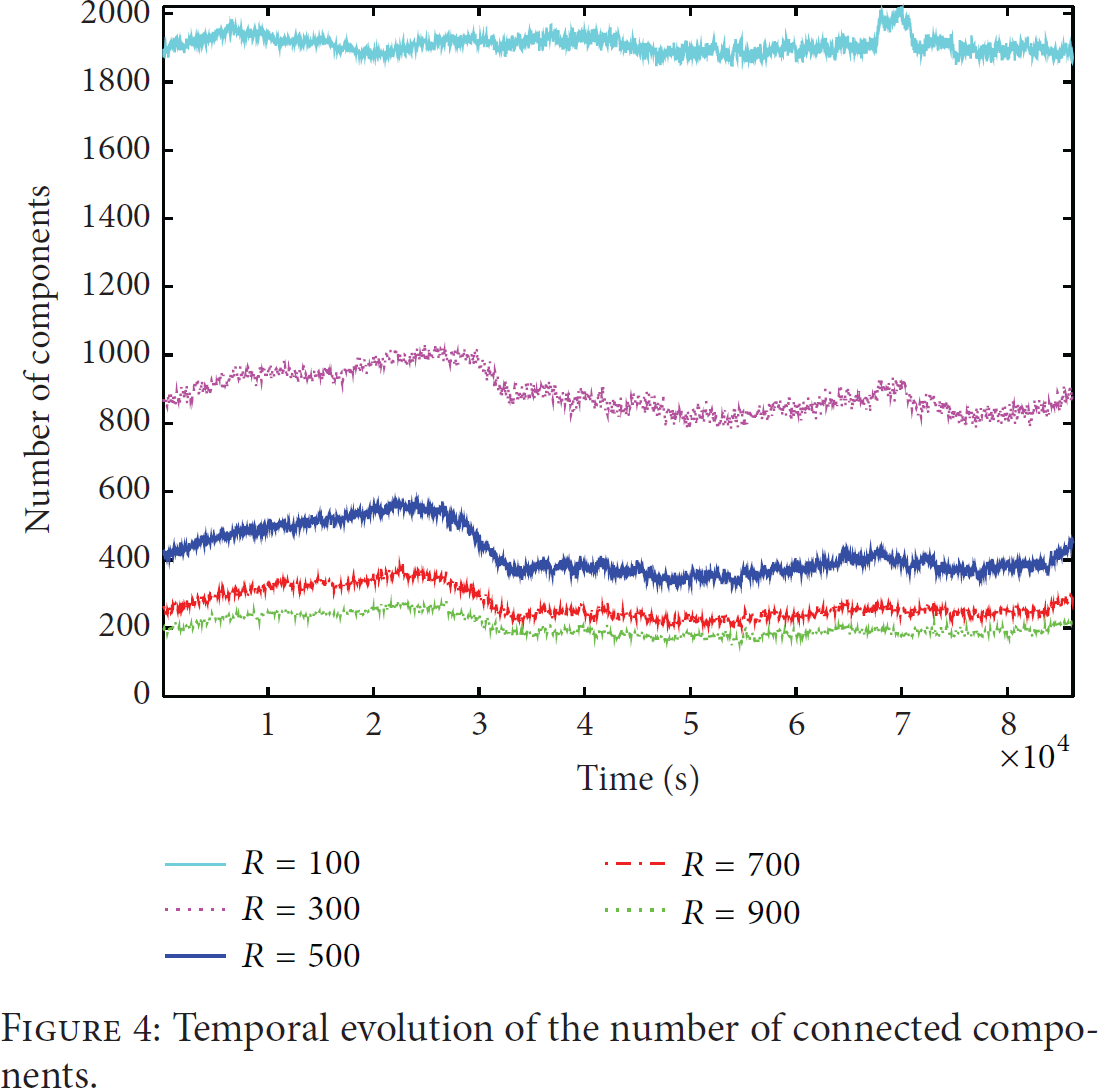
Temporal evolution of the number of connected components.

Figure 5

The average number of the connected components versus transmission radius.

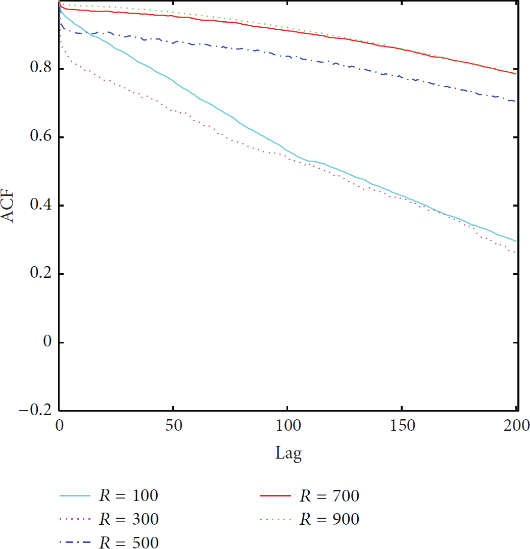
It is often suggested that a more quantitative way to view time evolution is proposed to look at the autocorrelations of the number of components. The theoretical autocorrelation function (hereafter, ACF) is defined as follows: $c o r r (C (t), C (t - k)) = c o v (C (t), C (t - k)) / \sqrt{v a r (C (t))} \sqrt{v a r (C (t - k))}$ , where $c o v (C (t), C (t - k))$ is the autocovariance and $v a r (C (t))$ is the variance. Figure 6 are plots of the autocorrelation functions of the number of components. It is easy to see that the autocorrelation functions do exhibit a much slower decay behaviour except $R = 100 m$ . We conclude that the number of components themselves do show the evidence of temporal correlations and long-range dependency. Therefore, the short-range dependent processes such as the exponential, normal, or Poisson distributions cannot capture the distribution characteristics.

Figure 6

The ACF for the number of connected components.

The short-range dependent processes cannot capture the distribution characteristics of the number of connected components. Which distribution function can describe the statistical characteristics of the number of connected components in general? We use kernel density estimation (KDE) methods to estimate the density of the number of connected components. 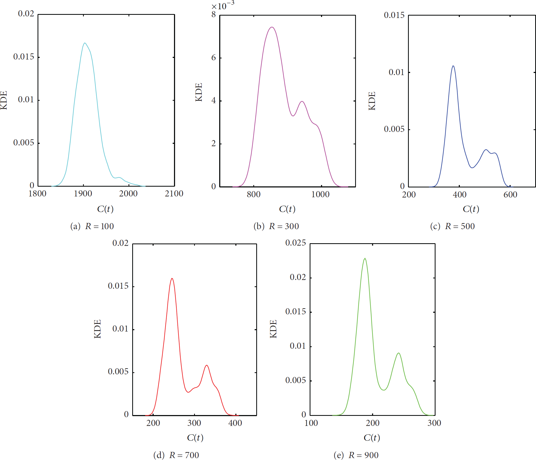From Figure 7, we can see that almost all the number of connected components exhibits new probability density function with several different shapes including bimodal shape except $R = 100 m$ . In statistics, a bimodal distribution is a continuous probability distribution with mixture of two different unimodal distributions. Therefore, the number of connected components cannot be described by unimodal distributions.

Figure 7

The kernel density of the number of connected components time series.

4.2. Giant Component and Connectivity Probability

Not only the availability but also the reliability of large components is a critical factor for the design of vehicular network solutions. Figure 8 illustrates the size of the giant component over time for different transmission radius. Figure 8 plots the average connectivity probability as a function of transmission radius. From Figures 8 and 9, we can see that almost no giant components appear during 24 hours when $R = 100 m$ . Even when $R = 300 m$ , not only the giant component is less probable to appear, but it never includes more than 18% of the network vehicles. The average size of giant components of total vehicles is 6.71%. When the radius increases from 300 m to 700 m, the connectivity probability relies on linear growth. Conversely, when the transmission radius is larger than 700 m, the giant component keeps stable and even contains 70% to 80% of the vehicles.

Figure 8

Temporal evolution of the size of giant component.

Figure 9

The average connectivity probability versus transmission radius.

Furthermore, we examine the evolution of the giant component over time. The autocorrelation function (ACF) of the size of giant component time series for different transmission radius is shown in Figure 10. Their autocorrelation functions for different R show a slowly decaying tail and remain significantly positive over many time lags. We conclude that the size of giant component exhibits strong temporal correlations and long-range dependency. We also use kernel density estimation methods to estimate the density of the size of giant component. From Figure 11, we can see that almost all the sizes of giant component exhibit new probability density function with several different shapes including bimodal shape. The size of giant component cannot be described by unimodal distributions.

Figure 10

The ACF for the size of giant component.

Figure 11

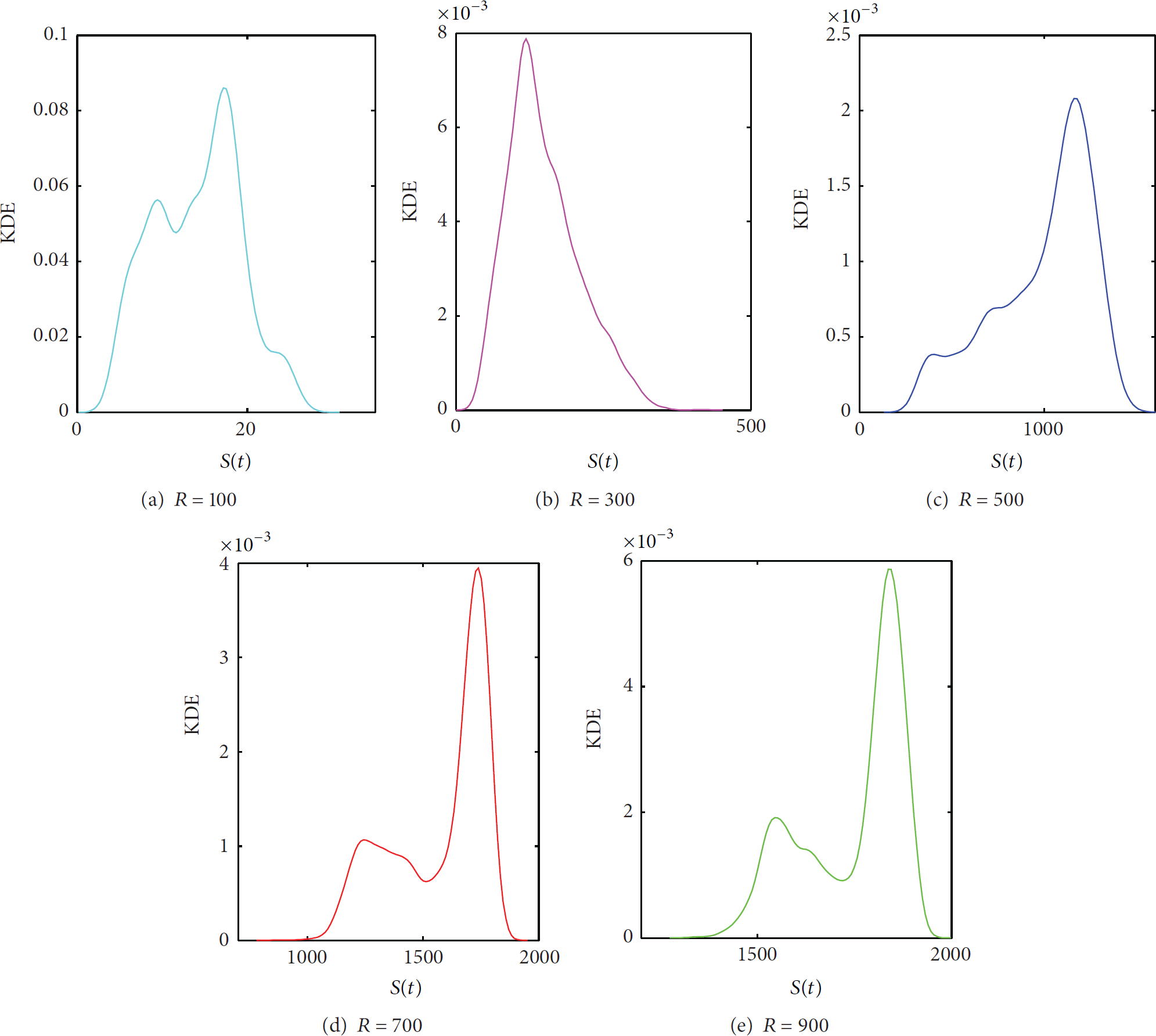
The kernel density of the size of giant component time series.

Key Networking Insights. Comparing Figure 4 with Figure 5 and Figure 8 with Figure 9, although we can conclude that the whole topology of the VANETs is broken into a large number of small-sized connected components, the giant component can cover a large number of vehicles. Moreover, the giant component keeps stable when transmission radius reaches the threshold. Therefore, on the one hand, if the giant component keeps stable, we can make use of this feature by keeping important information on the vehicles in the giant component and design strategies to forward the information with the giant component. On the other hand, we consider that roadside unit (RSU) deployment is critical to achieve large components of the connected vehicles. In particular, RSUs should be deployed where weak ties tend to appear, so as to act as permanent bridges among small but stable connectivity islands. The problems about optimization of RSUs deployment and transmission radius will be developed in our future work.

4.3. Connectivity Length

The connectivity length over time is reported in Figure 12. When the transmission radius increases from 100 m to 900 m, the average connectivity length decreases sharply from 5108.9 to 13.5447. Figure 13 suggests that the connectivity length is strongly affected by transmission radius. The relationship between the average connectivity length and transmission radius can be quite well fitted by the power-law distribution function $\bar{D} (R) = a R^{b}$ as the coefficients $a = 3.134 e + 008$ and $b = - 2.394$ of which the 95% confidence bounds are $(- 8.856 e + 007,7.153 e + 008)$ and $(- 2.672, - 2.116)$ correspondingly. And the goodness of the fitting parameters is as follows: 4703 (SSE), 0.9998 (R-square), 0.9997 (adjusted R-square), and 39.59 (RMSE).

Figure 12

Temporal evolution of the connectivity length.

Figure 13

The average connectivity length versus transmission radius.

Though the transmission radius is large ( $R = 900 m$ ), the average global efficiency is 0.0762. This means that the efficiency of the global communication in VAENTs is low. This result shows that VANET is not small-world networks since the small-world networks have high global efficiency, that is, are very efficient in global communication.

Figure 14 is plots of the autocorrelation functions of the connectivity length. The strong temporal correlation of the connectivity length time series can be observed for any R in Figure 13. In particular, when the signal transmission radius is over 700 m, the global efficiency appears to be almost the same correlation coefficient. The slowly decaying autocorrelation function implies that the global efficiency possesses a strong temporal correlation and long-range dependence across various transmission radius. Moreover, the connectivity length also cannot be described by unimodal distributions.

Figure 14

The ACF for the connectivity length.

We analyze the influence of various time windows on evolution of the connectivity parameters. The ACF of the connectivity parameters such as the number of connected components, the size of giant component, and the connectivity length is reported in Figures 15(a), 15(b), and 15(c), respectively, where we set the signal transmission radius as 300 m. As shown in Figure 15(a), with the time window increasing, the temporal correlation of the number of connected components is reducing quickly; that is, the smaller the time window is, the stronger the correlation is. Similar results are obtained for the size of giant component and the connectivity length as well.

Figure 15

The ACF for connectivity parameters under different time windows.

5. Conclusion

In this paper, we analyzed the evolution of the connectivity for VANETs based on real taxi GPS traces in Shanghai. We found that the number of the connected component, the size of the giant component, and the connectivity length time series possess strong temporal correlation and long-range dependence. The short-range dependent processes such as the exponential, normal, or Poisson distributions cannot capture the statistical distribution characteristics. Moreover, all connectivity parameters cannot be described by unimodal distributions. The relationship between the average number of components and the transmission radius is similar to the relationship between average connectivity length and transmission radius in that it is described by a power-law function. We also found that, by adopting a reasonable communication range, the size of the giant component is stable. These results will be significant to optimize the RSUs deployment and transmission radius to keep the giant component stable and design more efficient strategies to forward the information in VANETs.

Our study still has limitations that open the way for our future research activities. First, our analysis is based on taxi GPS data collected in Shanghai urban area. Shanghai is the largest city by population in China. Compared with the city size, the taxi GPS data is relatively smaller. In our future work, we plan to investigate the connectivity evolution for networks where all the vehicles in Shanghai's urban areas will be contained by validated microscopic mobility models. Second, our connectivity analysis builds on a unit-disc representation of the radio signal propagation. Considering some model of signal fading would add the rapid variability induced by radio signal fluctuations on top of the connectivity dependent dynamics we observe in our study. Third, in this paper we only investigate the evolution of the instantaneous network connectivity. The temporal connectivity of vehicular delay-tolerant networks is very important for data dissemination. Therefore, we will provide the extension of our work based on more accurate temporal models.

Footnotes

Conflict of Interests

The authors declare that there is no conflict of interests regarding the publication of this paper.

Acknowledgments

This work was supported in part by the NSFC under Grants nos. 61363081 and 71561024, the NSF of Gansu Province under Grants nos. 1308RJZA294 and 1506RJZA121, and the Fundamental Research Funds for the Gansu Universities.

References

Toor

Muhlethaler

Laouiti

Fortelle

Vehicular ad hoc networks: applications and related technical issues

IEEE Communications Surveys and Tutorials 2008 10 3 74 88

Yousefi

Mousavi

M. S.

Fathy

Vehicular Ad hoc networks (VANETs): challenges and perspectives

Proceedings of the 6th International Conference on ITS Telecommunications Proceedings (ITST ′06)

June 2006

Chengdu, China

IEEE

761 766

10.1109/itst.2006.289012

2-s2.0-44449175231

Katuka

J. I.

Muhammad

S. A. L.

VANETs and its related issues: an extensive survey

Journal of Theoretical & Applied Information Technology 2014 66 1 547 563

Yousefi

Altman

El-Azouzi

Fathy

Analytical model for connectivity in vehicular Ad Hoc networks

IEEE Transactions on Vehicular Technology 2008 57 6 3341 3356

10.1109/TVT.2008.2002957

2-s2.0-57049173375

Chandrasekharamenon

N. P.

Ancharev

Connectivity analysis of one-dimensional vehicular ad hoc networks in fading channels

EURASIP Journal on Wireless Communications and Networking 2012 2012, article 1 16

10.1186/1687-1499-2012-1

2-s2.0-84872867063

Ganti

R. K.

Haenggi

Dynamic connectivity and path formation time in Poisson networks

Wireless Networks 2014 20 4 579 589

10.1007/s11276-013-0620-y

2-s2.0-84899653226

Zhuang

Pan

Cai

A probabilistic model for message propagation in two-dimensional vehicular ad-hoc networks

Proceedings of the 7th International Workshop on Vehicular Ad Hoc Networks

September 2010

ACM

31 40

10.1145/1860058.1860064

2-s2.0-78649258156

Zhang

Sun

Pan

Connectivity analysis for vehicular ad hoc network based on the exponential random geometric graphs

Proceedings of the 25th IEEE Intelligent Vehicles Symposium (IV ′14)

June 2014

Dearborn, Mich, USA

IEEE

993 998

10.1109/ivs.2014.6856464

2-s2.0-84905389234

Cheng

Panichpapiboon

Effects of intervehicle spacing distributions on connectivity of VANET: a case study from measured highway traffic

IEEE Communications Magazine 2012 50 10 90 97

10.1109/mcom.2012.6316781

2-s2.0-84867158219

10.

Conceição

Ferreira

Barros

A cautionary view of mobility and connectivity modeling in vehicular ad-hoc networks

Proceedings of the IEEE 69th Vehicular Technology Conference (VTC ′09)

April 2009

Barcelona, Spain

1 5

10.1109/vetecs.2009.5073286

2-s2.0-70349690757

11.

Ivan

W. H. H.

North

R. J.

Polak

J. W.

Leung

K. K.

Impact of transport models on connectivity of vehicular ad-hoc networks

Proceedings of the 12th World Conference on Transport Research

July 2010

Lisbon, Portugal

1 25

12.

Hammouda

Tounsi

Frikha

Towards a study of mobility models impact on VANET connectivity metrics

Proceedings of the 3rd International Conference on the Network of the Future (NOF ′12)

November 2012

Gammarth, Tunisia

IEEE

1 5

10.1109/nof.2012.6463998

2-s2.0-84874677176

13.

Pallis

Katsaros

Dikaiakos

M. D.

Loulloudes

Tassiulas

On the structure and evolution of vehicular networks

Proceedings of the IEEE International Symposium on Modeling, Analysis and Simulation of Computer and Telecommunication Systems (MASCOTS ′09)

September 2009

London, UK

1 10

10.1109/mascot.2009.5366230

2-s2.0-76349118734

14.

Naboulsi

Fiore

On the instantaneous topology of a large-scale urban vehicular network: the cologne case

Proceedings of the 14th ACM International Symposium on Mobile Ad Hoc Networking and Computing

August 2013

Bangalore, India

ACM

167 175

10.1145/2491288.2491312

2-s2.0-84882989886

15.

Grzybek

Gregoire

Seredynski

Pascal

Evaluation of dynamic communities in large-scale vehicular networks

Proceedings of the 3rd ACM International Symposium on Design and Analysis of Intelligent Vehicular Networks and Applications (DIVANet ′13)

2013

Barcelona, Spain

93 100

16.

Ferreira

Conceiçao

Fernandes

Tonguz

O. K.

Urban connectivity analysis of VANETs through stereoscopic aerial photography

Proceedings of the IEEE 70th Vehicular Technology Conference Fall (VTC-Fall ′09)

September 2009

Anchorage, Alaska, USA

1 3

10.1109/vetecf.2009.5378962

2-s2.0-77951439720

17.

Glacet

Fiore

Gramaglia

Temporal connectivity of vehicular networks: the power of store-carry-and-forward

Proceedings of the IEEE Vehicular Networking Conference (VNC ′15)

December 2015

Kyoto, Japan

18.

Chen

Shi

Xiao

Empirical study on spatial and temporal features for vehicular wireless communications

EURASIP Journal on Wireless Communications and Networking 2014 2014, article 180

10.1186/1687-1499-2014-180

2-s2.0-84919910616

19.

Kim

Anderson

Temporal node centrality in complex networks

Physical Review E 2012 85 2 8

026107

10.1103/physreve.85.026107

2-s2.0-84863116426

20.

Simard

Nadeau

Kröger

Fastest learning in small-world neural networks

Physics Letters, Section A: General, Atomic and Solid State Physics 2005 336 1 8 15

10.1016/j.physleta.2004.12.078

ZBL1136.68504

2-s2.0-13144282731

21.

Zhu

Chang

Naik

Shen

Exploiting temporal dependency for opportunistic forwarding in urban vehicular networks

Proceedings of IEEE INFOCOM

April 2011

Shanghai, China

2192 2200

10.1109/infcom.2011.5935032

2-s2.0-79960860837

22.

Deakin

R. E.

Hunter

M. N.

Karney

C. F. F.

The Gauss-Krüger projection

Proceedings of the 23rd Victorian Regional Survey

September 2010

23.

Jiang

Chen

Delgrossi

Optimal data rate selection for vehicle safety communications

Proceedings of the 5th ACM International Workshop on Vehicular Ad Hoc Networks (VANET ′08)

September 2008

San Francisco, Calif, USA

30 38

10.1145/1410043.1410050

24.

ASTM

Standard specification for telecommunications and information exchange between roadside and vehicle systems—5 GHz band Dedicated Short Range Communications (DSRC) Medium Access Control (MAC) and Physical Layer (PHY) specifications

ASTM 2010 E2213-03

West Conshohocken, Pa, USA

ASTM International

An Empirical Study on Evolution of the Connectivity for VANETs Based on Taxi GPS Traces

Abstract

1. Introduction

2. Methodology

2.1. Temporal Networks Model

2.2. Connected Component

2.3. Giant Component and Connectivity Probability

2.4. Connectivity Length

3. Real Vehicle Mobility Traces

4. The Evolution of VANETs Connectivity

4.1. Connected Component

4.2. Giant Component and Connectivity Probability

4.3. Connectivity Length

5. Conclusion

Footnotes

Conflict of Interests

Acknowledgments

References