Low Power OFDM Receiver Exploiting Data Sparseness and DFT Symmetry

Abstract

An undersampling technique appropriate for Orthogonal Frequency Division Multiplexing (OFDM) that can be implemented with low complexity hardware is presented. The OFDM receiver can operate in undersampling mode, 75% of the time. One of the advantages of the proposed scheme is the reduction down to the half of the power consumed by the Analog Digital Converter (ADC) and the Fast Fourier Transform (FFT). The FFT memory requirements for sample storage can also be reduced and its operating speed can be increased. Simulations were performed for two Quadrature Amplitude Modulation orders (16-QAM and 32-QAM), two options for the FFT size (1024 and 4096), two alternative input symbol structures for the inverse FFT (IFFT), and several sparseness levels and samples substitution options. The Symbol Error Rate (SER) and image reconstruction examples are used to show that a full reconstruction or a very low error can be achieved. Although the proposed undersampling method is evaluated for wired channel, it can also be used without any modification to wireless Single Input Single Output (SISO) systems (with an expected SER degradation). It can also be used with Multiple Input Multiple Output (MIMO) systems when an appropriate arrangement of the IFFT input symbols is adopted.

1. Introduction

The OFDM is a popular modulation scheme in the contemporary telecommunication standards (like the IEEE 802.11 and 802.15 standards). The information exchanged over the OFDM transceivers may be occasionally sparse. However, the hardware of these systems does not usually take advantage of this fact in order to reduce its power consumption and the dynamic memory requirements during the time intervals where the transferred data are sparse. In this paper, the data sparseness is defined as the fraction S of the nonzero data bits ( $S\ll 1$ ). The proposed method can be used when sparse information transfer is detected in order to deactivate several power and time consuming operations and to avoid sampling some redundant input samples (by lowering the ADC sampling rate) on the receiver side. The real time adaptation of these operating features can be controlled by low complexity hardware.

The sampling rate of a signal has to be at least twice as high as its higher frequency component according to the Nyquist and Shannon theorems in order to avoid distortion and information loss. Nevertheless, fewer samples can be used if the information exchanged is sparse or compressible. If for example, the information is transmitted through a high frequency carrier, there is no need to use a sampling rate twice as high as the carrier frequency at the receiver. A sampling rate comparable to the information rate can be adopted instead. A common practice is to use an analog frequency downconversion step that generates an intermediate frequency signal that can be sampled at a rate close to the original information rate.

A popular method that can be used for the reconstruction of the original sparse data from fewer samples is the Compressive Sampling (or Compressed Sensing, CS for short) [1, 2]. The information recovery is based on optimization problems that can be solved by iterative procedures. The proposed hardware implementations of the CS techniques have often been based on DSP processors [3, 4] since the resources required are high if, for example, reconfigurable hardware is employed [5]. Kalman filters [6] have also been proposed for input signal correction and compared to CS techniques. The interpolation [7, 8] can also be viewed as a method that can reconstruct an input signal from fewer samples. The CS techniques have been employed in OFDM environments for the use of fewer pilot symbols and efficient bandwidth exploitation. However, no CS or other undersampling techniques have been proposed for the reconstruction of the original data instead of the pilot information in OFDM systems. This is due to the fact that the inherent data sparseness is cancelled out in such an environment by the interleaving scheme, the Forward Error Correction (FEC) encoding as well as the Fourier and inverse Fourier transforms that are applied.

A deterministic undersampling approach that is not modeled as an optimization problem is proposed for OFDM environments in [9]. This approach is based on the properties of the Discrete Fourier Transform (DFT) and it requires (a) an appropriate interleaving/deinterleaving scheme, (b) a data sparseness detector, (c) a simple digital control of the ADC sampling rate, and (d) a digital control for the deactivation of some FFT operations and sample storage since several FFT butterfly outputs are zero when the proposed undersampling method operates on sparse data. The hardware circuitry that implements the operations (a)–(d) listed above has a low complexity since there is no iterative or recursive operation. Thus, no additional latency is introduced and finally no high precision arithmetic operations are required.

In our previous approach [9], the maximum number of samples (R) that could be omitted and replaced by others that are already available is $N/4$ , where N is the number of points used by the FFT and the IFFT in the OFDM transceiver. In the current work, additional DFT properties are exploited in order to increase the number R by 50%, that is, to $3N/8$ without worsening the achieved BER. The new undersampling techniques introduced in this paper allow information recovery with low error even if the sparseness level of the input data is worse. For example, in [9] when $R=N/8$ and $S=2\%$ , the achieved BER was 10⁻² while the SER (which is expected to be worse than BER) falls close to 10⁻⁴ here under the same conditions. Moreover, an additional IFFT input structure is tested here; different conditions are simulated and image reconstruction is also used as a case study here. The improvement in the number of omitted and replaced samples has a direct impact to the power consumption of the OFDM implementation since all the critical parameters including the undersampling intervals, the number of deactivated FFT operations, and the memory storage requirements can be improved by a similar factor. The SER achieved can be zero in many cases or at least lower than 10⁻³ if the input data are sparse enough and a low-order QAM modulation is employed.

The appropriate OFDM environment is described in Section 2 while the proposed undersampling method is presented in Section 3. Simulation results from random input data and image processing are presented in Section 4 for a broad channel Signal to Noise (SNR) range, a number of different R values, various sparseness levels, QAM orders and FFT sizes.

2. OFDM Transceiver Description

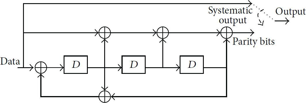
The input data stream at the OFDM transmitter is initially encoded in order to apply an efficient FEC decoding algorithm on the receiver side and correct the potential errors that will occur during the data transfer. The encoder is usually a Recursive Systematic Convolutional (RSC) encoder like the one presented in Figure 1. Such an encoder is characterized by a forward path (described by the polynomial $1+D+D^2+D^3$ ) and a feedback path (described by the polynomial $1+D+D^2$ ). The systematic output is connected directly to the input while the second output generates the parity bits. The parity bits are the necessary redundant information that has to be transmitted along with the original data for the error correction of as many errors as possible on the receiver side without the need of packet retransmission. The switch at the encoder outputs selects the current bit (either data or parity) that will drive the next transmitter stage, that is, the q-QAM modulator. A usual practice is to transmit in an alternative manner one data and one parity bit. However, a small buffering of a few bits ( ${\log }_2\left(q\right)$ ) is necessary in the proposed method since ${\log }_2\left(q\right)$ data or parity bits are mapped to a single QAM symbol.

Figure 1

The RSC encoder used.

The order of the forward and feedback encoder polynomials defines the minimum Trellis decoding diagram that will be needed on the receiver side in order to achieve an efficient correction scheme [10]. Taking into consideration that the input bit stream is sparse, the systematic data output of the encoder has a predictable value which is usually “0.” The parity output of an encoder like the one shown in Figure 1 is also “0” until the first “1” appears at the input. However, the feedback path of the encoder makes the effect of a single “1” at the input permanent at the parity output of the encoder.

In this paper, the fact that most of the initial parity output bits in a data packet have zero value since the first “1” at the data input may delay to appear is exploited first. If the input sparseness level is $S\hspace{0.17em}\hspace{0.17em}(S<1)$ , that is, if the fraction of nonzero values is S in an input data packet, then the first “1” will statistically appear at the position $1/S$ . For example, if the length of the input data packet is 1536 and $S=0.01$ (or 1%), then $1536·0.01\approx 15$ ones are expected to appear within this packet. If it is assumed that these 1's are uniformly scattered, then the first of them is expected to appear approximately at the position $1536/15\approx 102$ which is equal to $1/S$ . This example is simply used in order to show that if the first “1” delays to appear in a data packet, then the parity bits at the FEC encoder output will remain 0 for a long time interval. More specifically, the parity bits that correspond to the first 102 data bits with value 0 will also be zero (assuming of course that the FEC encoder is reset at the beginning of each packet transmission). Smarter parity bit pattern predictions are also employed since the same parity pattern is generated repeatedly by the FEC encoder between two consecutive appearances of “1” at its input. For example, after the first “1” at the input of the FEC encoder of Figure 1, the parity output generates the repeating pattern “1001110.”

At the next stage, the q-QAM takes place and ${\log }_2\left(q\right)$ bits are mapped to a q-QAM symbol. The parity and data bits are QAM modulated separately producing data QAM and parity QAM symbols. Most of the data QAM symbols will have an identical value $X_c$ . However, several parity QAM symbols generated at the beginning of a data packet encoding will also have the same value. Pad and Pilot symbols will also be added or merged with the data and parity QAM symbols to form the input of the IFFT (symbols $X_k$ , $0\le k<N$ ) that has to take place on the OFDM transmitter side. A Serial to Parallel converter can group the N, $X_k$ symbols before the IFFT is applied. As will be explained in the next section, it is desirable to have as many identical values at the odd positions of the IFFT input as possible. For this reason, the IFFT input can have the forms presented in Figure 2 for two IFFT/FFT sizes: $N=1024$ and $N=4096$ . Four pilots have been used with $N=1024$ and sixteen with $N=4096$ . The value selected for the pad and pilot symbols is equal to $X_c$ . The placement of the various symbols in Figures 2(a) and 2(b) is performed in such a way that the odd positions of the IFFT input are filled with data, pilot, or pad QAM symbols. In order to achieve this goal, the order of the parity and data QAM symbols is reversed after subsequent pilots. An appropriate IFFT input structure that can be used by the extended undersampling method described in the next section appears in Figure 2(c). The pilot or pad symbols can be placed either in the position of the data or the parity symbols. If the value of a pilot or pad symbol is selected to be equal to the predicted data or parity one, the error rate will not be significantly affected.

Figure 2

IFFT input packet structure for $N=1024$ (a) and $N=4096$ (b). Symbols “pilt” and “par” stand for pilot and parity QAM symbols, respectively. IFFT input packet structure appropriate for parity prediction (c).

The required interleaving can be performed before the IFFT, as bit interleaving between data bits only and parity bits only. Channel interleaving can also be performed by permuting data or parity QAM symbols as long as they are finally placed in odd and even positions, respectively.

The IFFT output symbols $x_n\hspace{0.17em}\hspace{0.17em}\left(0\le n<N\right)$ are serialized by a Parallel to Serial module while a Cyclic Prefix (CP) is transmitted before these IFFT output symbols in order to avoid intersymbol interference. The IFFT output and the CP are serially transmitted over the communication channel after their value is converted to an analog signal by a Digital to Analog Converter (DAC). The channel is assumed to be an Additive White Gaussian Noise (AWGN) channel which is appropriate for wired communications. However, the proposed architecture can be directly used in wireless environments too, with a single transmitter and a single receiver (SISO). Extensions of this architecture could also be employed in MIMO environments, but different IFFT input structures than the ones presented in Figure 2 may have to be selected to exploit Fourier properties when for instance antenna diversity is used. This is part of our on-going work.

The reverse procedure has to take place on the receiver side. A pair of ADCs can provide, through a Serial to Parallel module, the N digitized complex values that form the input of the FFT. In the case where no errors occur, the FFT output is the set of $X_k$ , q-QAM symbols. These q-QAM symbols are transformed to a symbol stream by a Parallel to Serial converter and then they are deinterleaved and assigned to a sequence of data and parity bits that are decoded by an appropriate FEC method like Viterbi, LDPC, Turbo Decoder, and so forth.

Except for the interleaving and the QAM symbol placement scheme that has already been described, the ADC and FFT stages of the receiver have also to be modified in the current OFDM framework. More specifically, the ADC sampling should be controlled by a simple digital circuit that will lower the sampling rate at predetermined time intervals when sparse data are detected at the input. A simple frequency divider like a flip flop can be employed to control the sampling rate of the ADC, since, for example, the sampling rate can be reduced to the half in the undersampling intervals if $N/4$ or $3N/8$ samples are substituted as will be described in the next section. If an ADC operates at the half sampling frequency the power consumed by the ADC is also expected to be reduced to the half [11]. The samples that have been omitted by the ADC sampling when it operates in lower rate are substituted by other already available samples that are expected to have the same value and can be temporarily stored in a buffer. The sparse data detector on the receiver side can be based on counting zeros in a frame payload after the FEC decoder. If the number of zeros is higher than a threshold the receiver recognizes a sparse data transmission and enters the undersampling mode. The end of the sparse data transmission can be detected at a higher network layer (like the transport layer) when a large number of errors are detected. In this case, the receiver exits the undersampling mode. The sparse data detector will also control the deactivation of specific FFT operations as described in [9].

3. The Undersampling Procedure

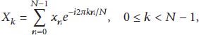
The DFT and the inverse DFT transforms are defined by the following equations, respectively,

$$\begin{array}{cc}& X_k={{\displaystyle \sum }}_{n=\mathrm{0}}^{N-\mathrm{1}}{x}_n{e}^{-i\mathrm{2}\pi kn/N},\hspace{1em}0\le k<N-\mathrm{1},\end{array}$$

(1)

$$\begin{array}{cc}& x_n=\frac{\mathrm{1}}{N}{{\displaystyle \sum }}_{k=\mathrm{0}}^{N-\mathrm{1}}{X}_k{e}^{i\mathrm{2}\pi kn/N},\hspace{1em}0\le n<N-\mathrm{1}.\end{array}$$

(2)

The undersampling policy followed in [9] has been based on the fact that the products for odd $k\hspace{0.17em}\hspace{0.17em}(k<N/2)$ and $k+N/2$ in (1) sum up to the same result in both $x_n$ and $x_{n+N/2}$ if n is also odd:

$$\begin{array}{cc}& x_n={{\displaystyle \sum }}_{k=\mathrm{0}}^{N-\mathrm{1}}{X}_k{e}^{i\left(\mathrm{2}\pi /N\right)kn}={{\displaystyle \sum }}_{k=\mathrm{0,2},\dots ,N-\mathrm{2}}{X}_k{e}^{i\left(\mathrm{2}\pi /N\right)kn}+{{\displaystyle \sum }}_{k=\mathrm{1,3},\dots ,N/\mathrm{2}-\mathrm{1}}\left(X_k{e}^{i\left(\mathrm{2}\pi /N\right)kn}+X_{k+N/\mathrm{2}}{e}^{i\left(\mathrm{2}\pi /N\right)\left(k+N/\mathrm{2}\right)n}\right)={{\displaystyle \sum }}_{k=\mathrm{0,2},\dots ,N-\mathrm{2}}{X}_k{e}^{i\left(\mathrm{2}\pi /N\right)kn}+{{\displaystyle \sum }}_{k=\mathrm{1,3},\dots ,N/\mathrm{2}-\mathrm{1}}\left(X_k-X_{k+N/\mathrm{2}}\right)e^{i\left(\mathrm{2}\pi /N\right)kn},\end{array}$$

(3)

$$\begin{array}{cc}& x_{n+N/\mathrm{2}}={{\displaystyle \sum }}_{k=\mathrm{0}}^{N-\mathrm{1}}{X}_k{e}^{i\left(\mathrm{2}\pi /N\right)k\left(n+N/\mathrm{2}\right)}={{\displaystyle \sum }}_{k=\mathrm{0}}^{N-\mathrm{1}}{X}_k{e}^{i\left(\mathrm{2}\pi /N\right)kn}{e}^{i\left(\mathrm{2}\pi /N\right)k\left(N/\mathrm{2}\right)}={{\displaystyle \sum }}_{k=\mathrm{0}}^{N-\mathrm{1}}{X}_k{e}^{i\left(\mathrm{2}\pi /N\right)kn}{\left(-\mathrm{1}\right)}^k={{\displaystyle \sum }}_{k=\mathrm{0,2},\dots ,N-\mathrm{2}}{X}_k{e}^{i\left(\mathrm{2}\pi /N\right)kn}-{{\displaystyle \sum }}_{k=\mathrm{1,3},\dots ,N/\mathrm{2}-\mathrm{1}}\left(X_k{e}^{i\left(\mathrm{2}\pi /N\right)kn}+X_{k+N/\mathrm{2}}{e}^{i\left(\mathrm{2}\pi /N\right)\left(k+N/\mathrm{2}\right)n}\right)={{\displaystyle \sum }}_{k=\mathrm{0,2},\dots ,N-\mathrm{2}}{X}_k{e}^{i\left(\mathrm{2}\pi /N\right)kn}-{{\displaystyle \sum }}_{k=\mathrm{1},\dots ,N/\mathrm{2}-\mathrm{1}}\left(X_k-X_{k+N/\mathrm{2}}\right)e^{i\left(\mathrm{2}\pi /N\right)kn}.\end{array}$$

(4)

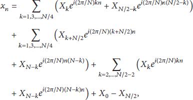
As can be seen, both (3) and (4) consist of a common term (the sum of the even k's) and a sum of differences for the odd k's. If $X_k=X_{k+N/\mathrm{2}}$ , then the second sum at (3) and (4) equals 0 and $x_n=x_{n+N/\mathrm{2}}$ for odd n values. This is why the structures of the IFFT input packets displayed in Figures 2(a) and 2(b) have been selected trying to place $X_k=X_c$ values at the odd k-positions. In this case, R of N, $x_n$ values, where R is up to $N/4$ (half of the $x_n$ symbols with odd n) can be substituted by others. $x_n$ symbols that will be used to substitute others can be copied directly by the Serial to Parallel module at the FFT input. For example, the $x_{n+N/\mathrm{2}}$ values with odd n and $n<N/2$ can be replaced by $x_n$ . Although the number of symbols used by the FFT on the receiver side is always N, large parts of these symbols are copies of others and do not need to be supplied by the ADC. Thus, the undersampling term used so far refers to the number of samples generated by the ADC that are lower than those determined by the Nyquist theorem. Of course, $X_k\ne X_{k+N/\mathrm{2}}$ for some odd k values since the input data are sparse but not zero and thus $X_k\ne X_c$ in these cases. As will be shown in the next section if $R=N/4$ then the achieved SER has an unacceptable error floor. However, if $R=N/8$ or lower and the sparseness level S is also low enough (below 1%), a good SER or even a full reconstruction can be performed.

In order to achieve an acceptable SER with higher R values, other DFT properties are also exploited in this paper. If we focus on $x_n$ and $x_{N/\mathrm{2}-n}$ with odd n and $n<N/4$ , (1) can be rewritten as

$$\begin{array}{cc}& x_n={{\displaystyle \sum }}_{k=\mathrm{1,3},\dots ,N/\mathrm{4}}\left(X_k{e}^{i\left(\mathrm{2}\pi /N\right)kn}+X_{N/\mathrm{2}-k}{e}^{i\left(\mathrm{2}\pi /N\right)n\left(N/\mathrm{2}-k\right)}\right)+{{\displaystyle \sum }}_{k=\mathrm{1,3},\dots ,N/\mathrm{4}}\left(X_{k+N/\mathrm{2}}{e}^{i\left(\mathrm{2}\pi /N\right)\left(k+N/\mathrm{2}\right)n}+X_{N-k}{e}^{i\left(\mathrm{2}\pi /N\right)n\left(N-k\right)}\right)+{{\displaystyle \sum }}_{k=\mathrm{2},\dots ,N/\mathrm{2}-\mathrm{2}}\left(X_k{e}^{i\left(\mathrm{2}\pi /N\right)kn}+X_{N-k}{e}^{i\left(\mathrm{2}\pi /N\right)\left(N-k\right)n}\right)+X_{\mathrm{0}}-X_{N/\mathrm{2}},\end{array}$$

(5)

where the first sum adds, in pairs, $X_k$ at odd positions that are symmetric around $N/4$ , the second sum adds the $X_k$ pairs with odd k, that are symmetric around $3N/4$ , and the last sum adds the $X_k$ pairs with even k, that are symmetric around $N/2$ .

After manipulating the exponents and taking into consideration the fact that n is odd everywhere while the k is either odd or even according to the specific sum that it is used in, (5) can be rewritten as

$$\begin{array}{cc}& x_n={{\displaystyle \sum }}_{k=\mathrm{1,3},\dots ,N/\mathrm{4}}\left(X_k{e}^{i\left(\mathrm{2}\pi /N\right)kn}-X_{N/\mathrm{2}-k}{e}^{-i\left(\mathrm{2}\pi /N\right)kn}\right)+{{\displaystyle \sum }}_{k=\mathrm{1,3},\dots ,N/\mathrm{4}}\left(-X_{k+N/\mathrm{2}}{e}^{i\left(\mathrm{2}\pi /N\right)kn}+X_{N-k}{e}^{-i\left(\mathrm{2}\pi /N\right)kn}\right)+{{\displaystyle \sum }}_{k=\mathrm{2},\dots ,N/\mathrm{2}-\mathrm{2}}\left(X_k{e}^{i\left(\mathrm{2}\pi /N\right)kn}+X_{N-k}{e}^{-i\left(\mathrm{2}\pi /N\right)kn}\right)+X_{\mathrm{0}}-X_{N/\mathrm{2}}.\end{array}$$

(6)

In the same way, $x_{N/\mathrm{2}-n}$ can be expressed as

$$\begin{array}{cc}& x_{N/\mathrm{2}-n}={{\displaystyle \sum }}_{k=\mathrm{1,3},\dots ,N/\mathrm{4}}\left(-X_k{e}^{-i\left(2\pi /N\right)kn}+X_{N/\mathrm{2}-k}{e}^{i\left(2\pi /N\right)kn}\right)+{{\displaystyle \sum }}_{k=\mathrm{1,3},\dots ,N/\mathrm{4}}\left(X_{k+N/\mathrm{2}}{e}^{-i\left(2\pi /N\right)kn}-X_{N-k}{e}^{i\left(2\pi /N\right)kn}\right)+{{\displaystyle \sum }}_{k=\mathrm{0,2},\dots ,N/\mathrm{2}}\left(X_k{e}^{-i\left(2\pi /N\right)kn}+X_{N-k}{e}^{i\left(2\pi /N\right)kn}\right)+X_{\mathrm{0}}+X_{N/\mathrm{2}}.\end{array}$$

(7)

As can be seen when (6) and (7) are compared, IFFT outputs $x_n$ and $x_{N/\mathrm{2}-n}$ are equal, if $X_k=X_{N/\mathrm{2}-k}$ (with odd k and k lower than $N/4$ ), $X_{k+N/\mathrm{2}}=X_{N-k}$ (with odd k and $N/2<k<3N/4$ ), and $X_k=X_{N-k}$ , with k being even and $0\le k<N/2$ . In other words, $x_n=x_{N/\mathrm{2}-n}$ if the following conditions hold: (a) $X_k$ symbol pairs at odd positions that are symmetric around $N/4$ are equal, (b) $X_k$ pairs with odd k that are symmetric around $3N/4$ are equal, and (c) $X_k$ pairs with even k that are symmetric around $N/2$ are also equal.

This has been proven for odd n values that are lower than $N/2$ but can also be proved in a similar manner for $x_n$ and $x_{N-n}$ , where n is again odd and $N/2<n<3N/4$ . The conditions (a) and (b) defined above hold for most of the symbol pairs in Figures 2(a) and 2(b), since data QAM symbols have been stored in the odd positions. It cannot be guaranteed though that most of the even positioned pairs will have identical samples since these are parity symbols. The fact that the initial parity symbols in a packet have also the same value $X_c$ as discussed in the previous section is used in this work in order to allow the substitution of additional samples at the receiver FFT. The fact that a parity pattern is repeated between successive 1's at the FEC encoder sparse input is exploited by the IFFT input structure shown in Figure 2(c) in order to reassure that the condition (c) is valid for more symbol pairs and thus a lower error can be achieved.

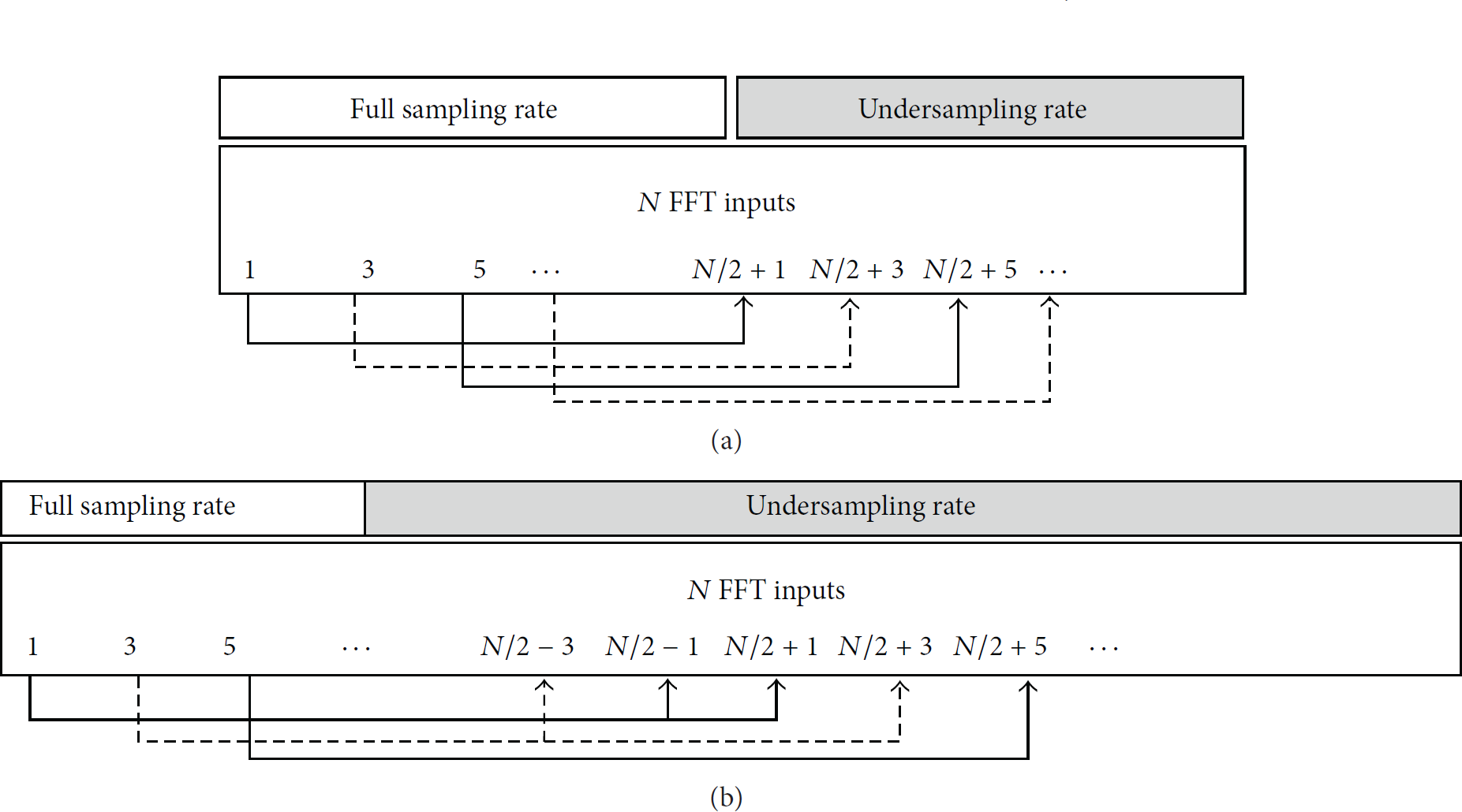
The undersampling interval can be extended using the previous conditions (a)–(c) as shown in Figure 3. Figure 3(a) shows that up to $N/4$ samples could have been substituted in [9]. More specifically, the sample $x_{N/\mathrm{2}+n}$ (n is odd) could have been omitted by the sampling procedure on the receiver side and its value could have been retrieved by $x_n$ . Now, the value of $x_{N/\mathrm{2}-n}$ can also be considered to be replaced by $x_n$ as shown in Figure 3. Consequently, the sampling interval can be extended by 50%. Fewer samples can be replaced if a better SER should be achieved, but the tradeoff between the substituted samples R and the achieved SER is still better than using the sampling interval shown in Figure 3(a) as will be shown in the following section. Fewer samples can be replaced if the ones that are omitted are selected with a distance of 4 or 8 instead of 2. For example, if the dashed lines of Figure 3(b) are not used then samples at a distance of 4 are selected for substitution.

Figure 3

Undersampling intervals applied in [9] (a) and the extended undersampling interval used in this work (b).

4. Simulation Results

The sample substitution policy is initially evaluated on raw data with various degrees of sparseness. In the simulations initially presented, a data bit stream is mapped to QAM symbols that form the input of an N-point IFFT. The sample substitution policy is applied to the output of the IFFT and the resulting set of data forms the input of an N-point FFT transform in order to reconstruct the initial QAM symbols and estimate the SER of this process. In this setup, the only error sources are the sample substitution process and the AWGN noise. The AWGN is expressed as the channel SNR in Figures 4–6. The truncation error of the real numbers is not taken into consideration and a perfect synchronization is assumed between the receiver and the transmitter.

Figure 4

$S=0.5$ % for $N=\mathrm{1024}/\text{16-QAM}$ (a) and $N=\mathrm{4096}/\text{32-QAM}$ (b).

Figure 5

$S=1$ %, $N=\mathrm{1024}/\text{16-QAM}$ (a) and $N=\mathrm{4096}/\text{32-QAM}$ (b).

Figure 6

$S=2$ %, $N=\mathrm{1024}/\text{16-QAM}$ (a) and $N=\mathrm{4096}/\text{32-QAM}$ (b).

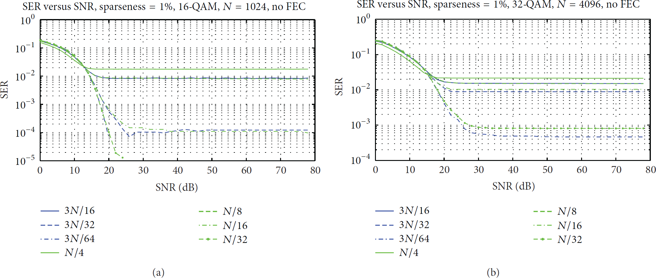
The IFFT input structures used are the ones shown in Figures 2(a) and 2(b). The sample substitution policies tested include $R=3N/16$ , $R=3N/32$ , and $R=3N/64$ for the new method proposed in this paper and $R=N/4$ , $R=N/8$ , $R=N/16$ , and $R=N/32$ for the policy followed in [9].

As can be seen from Figures 4–6, there are several cases where the new substitution policy achieves better SER although the number of samples replaced is higher. For example, in Figure 4(b), the case where $R=N/32$ shows a worse SER compared to the case of $R=3N/64$ , although the number of samples replaced in the latter case is higher by $N/64$ . The SER is worse for higher-order QAM. This stems from the fact that when more bits are mapped to a single QAM symbol, there is a higher probability that this symbol has been derived from bit combinations that contain 1's and thus its value will not be equal to $X_c$ . If the sparseness level is 1% or lower, there are several R values that generate acceptable SER. More specifically, for $R\le 3N/64$ , a full signal reconstruction can be performed in $N=1024/\text{16-QAM}$ combination for any sparseness level tested. For $R>N/16$ , the SER is not acceptable in most of the cases ( $\mathrm{S}\mathrm{E}\mathrm{R}>{10}^{-2}$ ).

In the new sample replacement policy, the SER is lower despite the fact that a higher number of R samples are substituted and this holds only when no FEC. If FEC method is employed (Viterbi) in order to emulate a full OFDM environment, the SER of the new method is much worse as can be seen from Figure 7 because it has been assumed that the parity QAM symbols have also the same value, $X_c$ . The SER can be improved if an FEC encoder with data rate higher than 1/2 is used, since most of the IFFT input frame positions will be allocated to data symbols. Moreover, the parity pattern prediction employed in Figure 2(c) allows the placement of identical symmetric parity symbols to comply with the condition (c) defined in Section 3.

Figure 7

$S=1$ %, Viterbi FEC applied, $N=\mathrm{1024}/\text{16-QAM}$ (a) and $N=\mathrm{4096}/\text{32-QAM}$ (b).

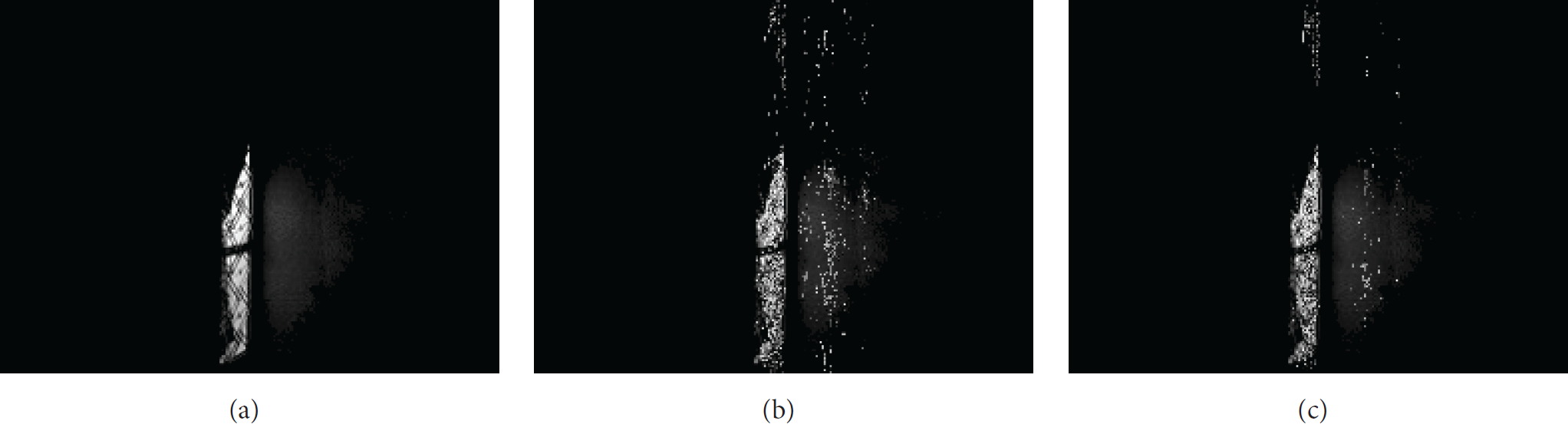
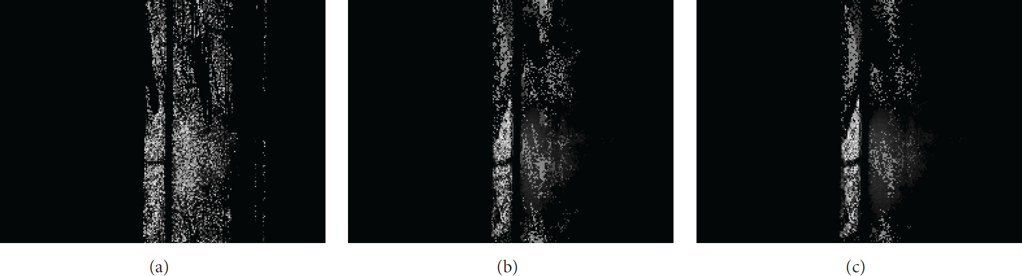
The last case study concerns the reconstruction (Figures 8–11) within an OFDM environment of two images. The original first image (A) is shown in Figure 8(a), and the reconstructed images using as IFFT input structure the one shown in Figure 2(a) appear in Figures 8(b), 8(c), and 9. The Mean Square Error (MSE) and Normalized MSE (NMSE) are listed in each case. The best NMSE = 0.085 is achieved when $N/32$ samples are substituted with the old undersampling method [9]. When $3N/64$ samples are substituted with the proposed method, NMSE is 0.109. It is interesting to notice that when $R=3N/32$ samples are replaced by the new undersampling method, the NMSE is 0.17 when FEC is used and falls below 0.125 when the FEC is deactivated.

Figure 8

Image reconstruction A: original (a), $R=N/16$ , MSE = 2.21, and NMSE = 0.105 (b), $R=N/32$ , and MSE = 1.78, and NMSE = 0.085 (c).

Figure 9

Image reconstruction A: $R=3N/16$ , MSE = 3.57, and NMSE = 0.17, with FEC (a), $R=3N/32$ , MSE = 2.62, and NMSE = 0.1248, no FEC (b), and $R=3N/64$ , MSE = 2.29, and NMSE = 0.109 (c).

Figure 10

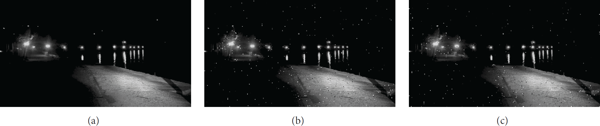
Image reconstruction B: original (a), $R=N/8$ , MSE = 0.81, and NMSE = 0.0125 (b), and $R=N/16$ , MSE = 0.145, and NMSE = 0.0022 (c).

Figure 11

Image reconstruction B: $R=3N/4$ , MSE = 7.215, and NMSE = 0.11 (a), $R=3N/8$ , MSE = 2.25, and NMSE = 0.039 (b), and $R=3N/16$ , MSE = 0.41, and NMSE = 0.0064 (c).

The original second image (B) is shown in Figure 10(a), while the reconstructed images are shown in Figures 10(b), 10(c), and 11. In the reconstruction of the second image, the Viterbi FEC decoding is used in all cases and the IFFT input structure shown in Figure 2(c) is employed. The exploitation of the advanced parity pattern predictability of this IFFT input structure leads to better MSE/NMSE results as can be seen by comparing, for example, the NMSE errors in the common cases between images A and B: $R=N/16$ and $R=3N/16$ . With $R=N/16$ , the NMSE in the reconstruction of images A and B is 0.105 and 0.0022, respectively. With $R=3N/16$ , the NMSE in the reconstruction of images A and B is 0.17 and 0.0064, respectively. A good quality image reconstruction can be achieved in Figures 10 and 11 even if a higher number of samples are omitted by the undersampling process (e.g., $R=N/8$ and $R=3N/16$ ).

In [2], a CS approach for surveillance applications is described showing NMSE higher than 0.11. In [6], the proposed Kalman filter for slowly changing sparse input patterns is compared to regular CS approaches achieving in some cases MSE lower than 0.21 and in some others an MSE between 10 and 22. The MSE in [8] is measured in dB and shows an error floor of −15 dB when the channel SNR is higher than 20 dB.

The number of samples required for the input signal reconstruction by the referenced approaches is smaller than the ones required by the proposed method. Nevertheless, complicated hardware is needed in order to solve the optimization problems used in these approaches. Although the number of samples required by the proposed undersampling method has been reduced in this paper concerning [9], it is still relatively high. However, it can be implemented with very low complexity hardware since no optimization problems and iterative processes are used. Moreover, no additional delay is introduced due to the noniterative nature of the proposed procedure. On the contrary, the FFT has been accelerated since many of its butterflies or operations can be deactivated when sparse data are used. Significant reduction can also be achieved in this way in the power and memory requirements of the final system.

5. Conclusions

An undersampling method that can be used in a wired or wireless OFDM environment was presented in this paper. It can reduce the samples needed at the receiver by up to 3/8. It can be implemented with very low complexity/cost hardware, while a significant power reduction (up to 1/2) can be achieved since the ADC at the receiver can slow down its sampling rate for up to 3/4 of the time. The simulation results showed that a better SER can be achieved, using the undersampling method proposed in this work in comparison with the method proposed in the past by the authors, although a higher number of samples can be substituted by others. In order to achieve this improvement, the parity QAM symbols must have a predictable value and this is feasible to a great extend when they are derived from sparse data.

Future work will focus on the improvement of the parity pattern prediction in order to achieve a lower error rate. Moreover, the proposed method will be implemented and tested in real applications.

References

1.
CandèsE. J.WakinM. B.An introduction to compressive samplingIEEE Signal Processing Magazine2008252213010.1109/msp.2007.9147312-s2.0-41949092318
2.
MahalanobisA.MuiseR.Object specific image reconstruction using a compressive sensing architecture for application in surveillance systemsIEEE Transactions on Aerospace and Electronic Systems20094531167118010.1109/TAES.2009.52591912-s2.0-72649100418
3.
TsaiY.-M.HuangK.-Y.KungH. T.VlahD.GwonY. L.ChenL.-G.A chip architecture for compressive sensing based detection of IC trojansProceedings of the IEEE Workshop on Signal Processing Systems (SiPS ‘12)October 2012Quebec, CanadaIEEE616610.1109/sips.2012.332-s2.0-84875287436
4.
TianJ.HuangY.Communication system with compressive sensingPCT2011WO2011047627A1
5.
StanislausJ. L. V. M.MohseninT.Low-complexity FPGA implementation of compressive sensing reconstructionProceedings of the International Conference on Computing, Networking and Communications (ICNC ‘13)January 2013San Diego, Calif, USA67167510.1109/iccnc.2013.65041672-s2.0-84877621867
6.
VaswaniN.Kalman filtered compressed sensingProceedings of the 15th IEEE International Conference on Image Processing (ICIP ‘08)October 2008San Diego, Calif, USAIEEE89389610.1109/icip.2008.47118992-s2.0-69949126538
TuncerT. E.Block-based methods for the reconstruction of finite-length signals from nonuniform samplesIEEE Transactions on Signal Processing200755253054110.1109/tsp.2006.885692MR24459632-s2.0-33847608773
9.
PetrellisN.Under-sampling in OFDM telecommunication systemsApplied Sciences2014417998
10.
PimentelC.SouzaR. D.Uchôa-FilhoB. F.BenchimolI.Minimal trellis for systematic recursive convolutional encodersProceedings of the IEEE International Symposium on Information Theory Proceedings (ISIT ‘11)August 2011Saint Petersburg, RussiaIEEE2477248110.1109/isit.2011.60340112-s2.0-80054797509