An Online-Traffic-Prediction Based Route Finding Mechanism for Smart City

Abstract

Finding fastest driving routes is significant for the intelligent transportation system. While predicting the online traffic conditions of road segments entails a variety of challenges, it contributes much to travel time prediction accuracy. In this paper, we propose O-Sense, an innovative online-traffic-prediction based route finding mechanism, which organically utilizes large scale taxi GPS traces and environmental information. O-Sense firstly exploits a deep learning approach to process spatial and temporal taxi GPS traces shown in dynamic patterns. Meanwhile, we model the traffic flow state for a given road segment using a linear-chain conditional random field (CRF), a technique that well forecasts the temporal transformation if provided with further supplementary environmental resources. O-Sense then fuses previously obtained outputs with a dynamic weighted classifier and generates a better traffic condition vector for each road segment at different prediction time. Finally, we perform online route computing to find the fastest path connecting consecutive road segments in the route based on the vectors. Experimental results show that O-Sense can estimate the travel time for driving routes more accurately.

1. Introduction

With the development of intelligent transportation technology in smart cities, finding fast driving routes can be widely used for traffic flow coordinating [1] to optimize the plan of traffic management and urban computing [2–5]. It is beneficial to find fast driving routes, which is conducive to energy saving and traffic congestion coordination.

The existing fastest routes finding approaches usually look into the real-time traffic conditions or infer potential travel costs of road through mining historical trajectory data. However, these works mostly assume the static travel cost on each road, while ignoring the potential temporal dynamics. In fact, the driving time, calculated from the current travel time of each road segment, deviates much from the truth. The soundness of fastest route finding relates greatly to the prediction accuracy of travel time for vehicles on the driving road. Hence, it is necessary to predict the traffic conditions of road segments at an appropriate future moment.

The urban traffic prediction usually utilizes historical and current traffic flow information to predict road conditions for future moments [6]. Most existing methods present prediction trends via statistics of the current road time-dependent evolution or they only work on spatial relationships between various segments without consideration of the temporal sequence and temporal-spatial information rules. Although available spatial-temporal information is combined to model the traffic network pattern in some previous works, this information does not play out its full potential. Traffic networks involve complicated relations in time and space. Specifically, traffic flow often contains high-dimensional, nonlinear, and nonstationary random data. In a previous work [7], a trained temporal-spatial deep learning approach DeepSense was proposed, which extracted features from the high-dimensional, nonlinear, and random traffic flow in large scale taxi GPS traces. However, we found that the prediction does not work so well at certain times, especially when there are insufficient taxi GPS traces. Based on this finding, it is proper to consider more factors such as environmental information containing temporal changes that influence the traffic flow of current road.

In this paper, we propose an online-traffic-prediction based route finding mechanism for smart city, namely, O-Sense. It comprehensively utilizes both temporal-spatial dynamic pattern in transportation network and temporally related environmental information to predict the travel cost of each route. Firstly, we analyze temporal and spatial information of taxi GPS traces via Restricted Boltzmann Machine (RBM) since it can process this information into low-dimensional features. Then the extracted low-dimensional data is put into a support vector machine (SVM) to gain a robust classifier that makes promise for the following prediction. Secondly, a linear-chain CRF predicts the future traffic state by giving the previous state in a temporal sequence and supplementary temporally related observations, since CRF is well known for being applied to mutually independent road segments. With auxiliary data utilized by CRF, prediction accuracy can be further enhanced through a dynamic weighted classifier fusion. Finally, using the results calculated from the predicted traffic conditions of each road, our system can perform the fast route selection for users.

The major contributions of this paper can be summarized into the following aspects.

• (1)

We propose an online-traffic-prediction based route finding mechanism O-Sense, which innovatively adopts a trained temporal-spatial deep learning approach. Significant traffic features can be extracted from the information synthesized from high-dimensional, nonlinear, and random large scale taxi GPS traces.

(2)

Combining temporally related environmental resources which are utilized in CRF as supplementary and dynamic weighted classifier fusion, the prediction accuracy can be further improved. As a result, taking full advantage of temporal and spatial information for traffic forecasting, it can effectively reflect the dynamic pattern shown in transportation network.

(3)

Utilizing large scale taxi GPS traces and environmental information in Wuhan, we evaluate the mechanism from a systematic perspective. Experimental results manifest that O-Sense mechanism can achieve sound and robust performance in prediction accuracy.

The remainder of this paper is organized as follows. Section 2 discusses related works. Section 3 presents the proposed O-Sense mechanism. Section 4 describes the processes of the traffic flow condition prediction. The performance of O-Sense is evaluated in Section 5. Finally, we make a conclusion in Section 6.

2. Related Works

2.1. Route Finding

Many works have been proposed for the fastest route finding problem, most of which can be divided into two categories based on the characteristics of the travel cost of road segments. On one hand, some works infer potential travel costs of road segments by exploiting historical trajectory data [8]. In [9], Tsuyoshi and Sugiyama treat the potential cost of each road as a spatial proximity-regularized trajectory regression problem. Gonzalez et al. find the fastest route based on the important driving and speed patterns which are learned from the historical trajectory data [10]. However, these works with the assumption of static travel costs cannot reflect the dynamic variances according to the actual traffic conditions. On the other hand, some works take the temporal dynamics of road travel costs into consideration to compute the fastest route [11]. Zheng and Ni learn the temporal dynamics of road travel costs, while it depends on integrated trajectories which cannot provide enough information when there is insufficient traffic information [12]. However, the pattern of the temporal dynamics of latent costs for road segments is hard to be predicted, especially in the cases with insufficient trajectory data.

2.2. Traffic Flow Condition Prediction

Most of the existing traffic flow condition prediction approaches merely utilize time-dependent traffic flow evolution rule for prediction. In [13], the autoregressive integrated moving average model (ARIMA) simply relies on historical traffic flow data of forecasted point taking temporal variation into consideration for prediction. The traffic flow prediction model based on $m_{\text{th}}$ -order Markov chain counts the transition probability of traffic flow state with historical data of forecasted road [14]. Coupled with current traffic situation and state transition probability, traffic condition in a period of time can be predicted. However, by using historical and real-time traffic patterns, the establishment of model in time sequence and the forecast duration is prolonged to some extent. Thus, there exists a lot of uncertainty and it is a statistical method. The variance-entropy-based clustering approaches [15] are used to estimate the travel time distribution in different time slots with historical data of object sites, which simply applies the idea of clustering analysis and generality.

There are also other methods that use spatial information in the transportation network to analyze the trend of traffic flow. Castro et al. [16] employ adjacent road information to forecast future traffic conditions, which does not take into account the influence of distant segments and temporal-spatial correlation of predicted road. Markov logic networks [17] have also been adopted to predict the traffic conditions at simultaneous locations in different future time.

The methods mentioned above merely model traffic flow trends with respect to one aspect. Temporal-spatial information has not been made use of to depict the characteristics of nonlinearity and randomness in the flow from an angle of the whole network. A Bayesian network approach [18] intended for traffic flow forecast integrates information of adjacent links and its spatial-temporal information in a transportation network. Sun and Zhang develop a selective random subspace predictor (SRSP) model [19] utilizing traffic flows of some most closely correlated links ranked by the measurement of Pearson correlation coefficient in the subspace to forecast the given road link. Although considering spatial-temporal information, these approaches did not extract the characteristics of high-dimension, nonlinearity, and randomness effectively.

3. O-Sense Overview

3.1. Preliminary

Definition 1 (route).

A route R is a group of consecutive road segments, R: $r_1\to r_2\to \cdots \to r_n$ , where $r_i$ is the ith road segment ( $1\le i\le n$ ). In route R, the end point of one road segment is the start point of its directly succeeding road segment; that is, $r_i.\text{end}=r_{i+\mathrm{1}}.\text{start}$ .

Definition 2 (taxi trajectory).

A trajectory is a time series of GPS points for a trip, where there is a geospatial coordinate set and a timestamp at each consecutive point.

Definition 3 (road segment/link).

A road link or segment is defined as a directed edge consisting of a direction symbol, two terminal points, and a length between crossroads.

Definition 4 (traffic flow condition).

We select traffic flow to denote traffic state of road segments. Given different speed situations and flow limits on distinct road segments, classified traffic state based on absolute speed is obviously inaccurate. According to the degree of traffic congestion, we can categorize the traffic conditions into five states, represented by $\Omega =\{\text{congesting}\mathrm{\hspace{0.17em}\hspace{0.17em}}(\text{Cg})$ ,   $\text{slow}\mathrm{\hspace{0.17em}\hspace{0.17em}}(\text{Sl}),\text{normal}\mathrm{\hspace{0.17em}\hspace{0.17em}}(\text{Nm}),\text{moderate}\mathrm{\hspace{0.17em}\hspace{0.17em}}\left(\text{Md}\right),\text{unimpeded}\mathrm{\hspace{0.17em}\hspace{0.17em}}(\text{Un})\}$ .

In detail, for the road segment R from 0 o'clock to 24 o'clock, a traffic flow $o_i$ is collected every time interval $\Delta t$ (e.g., 15 minutes), thus obtaining a series of traffic flow observations O (e.g., $o_1,o_2,o_3,\dots ,o_{96}$ ). In order to categorize these series to prementioned five states, we adopted K-means algorithm to cluster them into 5 subsets. By utilizing the average values of these 5 subsets, we can acquire their corresponding traffic states.

3.2. Framework

In order to learn online road travel costs for selecting the fastest routes for users, we propose an online-traffic-prediction based route finding mechanism, namely, O-Sense. As shown in Figure 1, to implement our mechanism for fastest route finding entails three procedures, namely, preprocessing, comprehensive feature learning, and route computing.

Figure 1

Architecture of O-Sense.

3.2.1. Preprocessing

Spatial trajectories collected by GPS-equipped vehicles are mapped onto a road network using a map-matching algorithm [20] and then stored into a taxi traces database. Environmental information is extracted to be used as temporally related features, as described in detail in Section 4.

3.2.2. Comprehensive Feature Learning

This process contains three parts: temporal-spatial feature deep learning, temporally related supplementary feature learning, and dynamic weighted classifier fusion. Firstly, to learn temporal-spatial features, we apply deep learning approach with preextracted temporal-spatial traffic flow information from taxi traces database. The trained temporal-spatial features are used to train RBM model, which is capable of predicting irregular and stochastic factors in traffic systems. By means of this trained model, the dimensionality and redundancy of the input features are reduced to a proper extent. The extracted features can be more effectively classified by a classification engine SVM. This engine is designed to utilize the extracted features to better train the expected prediction. Secondly, in order to learn supplementary temporally related features, CRF approach is trained to estimate the temporal state sequence of traffic flow with extracted environmental information. Therefore, the temporal state sequences obtained from CRF are matched for future traffic state prediction. The last technique adopted is dynamic weighted classifier fusion for comprehensively learning the whole temporal-spatial information and temporally related features. After real-time traffic flow data is preprocessed and temporally related features of forecasted time are preextracted, we can get an eventual prediction result. Details are presented in Section 4.

3.2.3. Online Route Computing

Given the prediction of each road segment at disparate time, a detailed route computing approach is performed in O-Sense to seek an optimal route. This approach utilizes the traffic condition of road segments in real-time for route computing. The process of online route computing is illustrated in Algorithm 1. In this paper, we consider the transportation networks exhibit the “FIFO” (First-In-First-Out) property; that is, if A and B visit node $n1$ at two different times $t1$ and $t2$ , where $t1\le t2$ , then A always arrives at node $n2$ before B for any arc $(n1,n2)$ . Our solution is composed of the following steps.

Algorithm 1: Online route computing algorithm.

Input: A directed graph $$G=\{V,E\},V=\{\mathit{1},\mathit{2},\dots ,n\}$$ , Departure time t

Output: The shortest distance from 1 to each node in G

Procedure:

(1) $$X=\{\mathit{1}\};Y=V-\{\mathit{1}\};\lambda [\mathit{1}]=\mathit{0}$$ ;

(2) for  $$x=\mathit{1}$$ to $$n-\mathit{1}$$

(3)  for  $$y=\mathit{1}$$ to n

(4)    if x is adjacent to y then $$r_{xy}[\mathit{60}]=\{r_{xy}[t],r_{xy}[t+\mathit{2}],\dots$$ ,

       $$r_{xy}[t+\mathit{120}]\}$$ ;

(5)    end if;

(6)  end for;

(7) end for;

(8) for  $$y=\mathit{2}$$ to n

(9)  if y is adjacent to 1 then $$\lambda [y]=r_{\mathit{1}y}[t]$$ ;

(10)    else $$\lambda [y]=\infty$$ ;

(11)     end if;

(12) end for;

(13) u = 1;

(14) for  $$j=\mathit{1}$$ to $$n-\mathit{1}$$

(15)    $$y\in Y,\lambda [y]$$ is the least among all values;

(16)    $$X=X\cup \{y\}$$ ;

(17)    $$Y=Y-\{y\}$$ ;

(18)   for every edge $$(y,w)$$

(19)    if $$w\in Y$$ and $$\lambda [y]+r_{yw}[t+r_{uy}[t]]<\lambda [w]$$ then

(20)       $$\lambda [w]=\lambda [y]+r_{yw}[t+r_{uy}[t]]$$ ;

(21)    end if;

(22)   end for;

(23)    $$t=t+r_{uy}[t]$$ ;

(24)    $$u=y$$ ;

(25) end for;

Step 1.

To find the fastest route with giving a starting point, a destination, and departure time, O-Sense firstly continually predicts a group of traffic states for each road segment that connects two points every two minutes for the following specific time period (e.g., for the following two hours). As the traffic condition division is based on specific clustering method, each traffic condition state takes a speed value as the clustering center. Hence, we can utilize five speed values to represent five states and they form a speed vector. Utilizing the speed vector to represent predicted traffic states, the weights of each road segment at different moments are obtained.

Step 2.

O-Sense chooses the optimal predicted value from the predicted speed vector of each road segment dynamically as the weight of corresponding road segment, which is closest to the actual value according to the time when the user arrives at the road segment. We can find the time-dependent fastest route using a modified Dijkstra algorithm [21, 22].

The fastest path connecting consecutive road segments is eventually found as we arrive at the destination. Owning to the different time costs of road segments, if we start at different time at the starting of the route even though given the same start point and destination, we may find disparate fast routes.

Example 1.

Seen from Figure 2, if starting at current time $t_{\text{ct}}$ from road intersection A, the road segment $r_{ab}$ of which the time cost $r_{ab}[t_{\text{ct}}]$ is the least in all road segments connecting A is chosen. Then the label of other nodes in the graph is updated, which denotes the shortest distance from the departure point to each node. When arriving at B, the time stamp at that time is $t_{\text{ct}}+r_{ab}[t_{\text{ct}}]$ . We compare the label of nodes C and E, that is, the travel time of going through $r_{be}$ and $r_{bc}$ ( $r_{be}[t_{\text{ct}}+r_{ab}[t_{\text{ct}}]]<r_{bc}[t_{\text{ct}}+r_{ab}[t_{\text{ct}}]]$ ) in this example. Then turn to E with updating the labels. Keeping searching like this, the fastest route from A to G starting at current time $t_{\text{ct}}$ is A → B → E → F → G. However, if starting at $t_{\text{ct}}+t_{\text{lr}}$ , where $t_{\text{lr}}$ denotes some time later than $t_{\text{ct}}$ , the route A →B → C → F → G now becomes the fastest rough route since when we arrive at B, the time stamp at that time is becoming $t_{\text{ct}}+t_{\text{lr}}+r_{ab}[t_{\text{ct}}+t_{\text{lr}}]$ and the travel time of going through $r_{be}$ is larger than that of $r_{bc}$ ; that is, $r_{be}[t_{\text{ct}}+t_{\text{lr}}+r_{ab}[t_{\text{ct}}+t_{\text{lr}}]]<r_{bc}[t_{\text{ct}}+t_{\text{lr}}+r_{ab}[t_{\text{ct}}+t_{\text{lr}}]]$ . Hence, our approach utilizes the traffic condition of road segments in real-time (when actually driven) for route computing.

Figure 2

Example of online route computing.

4. Comprehensive Feature Learning Based Prediction

This section details the methodology of the comprehensive feature learning based online traffic condition prediction mechanism, which consists of temporal-spatial feature deep learning, temporally related supplementary feature learning, and dynamic weighted classifier fusion-based comprehensive prediction.

4.1. Temporal-Spatial Traffic Feature Deep Learning

To simplify and reduce the dimension of the input data in order to efficiently learn the significant traffic features, O-Sense employs the temporal-spatial feature deep learning approach which includes three main steps: feature preextraction, feature learning, and training a SVM model.

4.1.1. Feature Preextraction

The correlation coefficient approach is first used to select the most correlated road segments between adjacent road segments and the predicted point, and then extracted features of these road segments are input into PCA to reduce data dimension and remove redundant information for better prediction.

Correlation Coefficient Approach. Considering N samples $\{x_i(k),y_j(t_{\text{ct}}+t_l)\}$     ( $i,j=\mathrm{1,2},\dots ,N$ ) in a spatial accessible space, $x_i(k)$ ( $k=\mathrm{1,2},\dots ,st$ ) represents the traffic flow of road segment i at time stamp k and $\bar{x}$ represents the mean value. And $y_j(t_{\text{ct}}+t_l)$ stands for the traffic flow of road segment j at predicted time $(t_{\text{ct}}+t_l)$ and $\bar{y}$ stands for the mean value, where $t_{\text{ct}}$ is the current time and $t_l$ means the duration of the prediction. The Pearson correlation coefficient $r_{ij}(k)$ between $x_i(k)$ and $y_j(t_{\text{ct}}+t_l)$ is defined as follows:

$$\begin{array}{ll}{r}_{ij}\left(k\right)& =\frac{{\sum }_{i=\mathrm{1}}^N\left(x_i\left(k\right)-\bar{x}\right)\left(y_j\left(t_{\text{ct}}+t_l\right)-\bar{y}\right)}{\sqrt{{\sum }_{i=\mathrm{1}}^N{\left(x_i\left(k\right)-\bar{x}\right)}^{\mathrm{2}}{\sum }_{i=\mathrm{1}}^N{\left(y_j\left(t_{\text{ct}}+t_l\right)-\bar{y}\right)}^{\mathrm{\hspace{0.17em}\hspace{0.17em}}\mathrm{2}}}}\\ & =\left(N{\displaystyle \sum }_{i=\mathrm{1}}^N{x}_i\left(k\right)y_j(t_{\text{ct}}+t_l)-{\displaystyle \sum }_{i=\mathrm{1}}^N{x}_i\left(k\right){\displaystyle \sum }_{i=\mathrm{1}}^N{y}_j(t_{\text{ct}}+t_l)\right)\\ & ·\left(\sqrt{N{\displaystyle \sum }_{i=\mathrm{1}}^N{x}_i{\left(k\right)}^{\mathrm{2}}-{\left({\displaystyle \sum }_{i=\mathrm{1}}^N{x}_i\left(k\right)\right)}^{\mathrm{2}}}\right.\\ & ·{\left.\sqrt{N{\displaystyle \sum }_{i=\mathrm{1}}^N{y}_j^{\mathrm{2}}\left(t_{\text{ct}}+t_l\right)-{\left({\displaystyle \sum }_{i=\mathrm{1}}^N{y}_j\left(t_{\text{ct}}+t_l\right)\right)}^{\mathrm{2}}}\right)}^{-1}.\end{array}$$

(1)

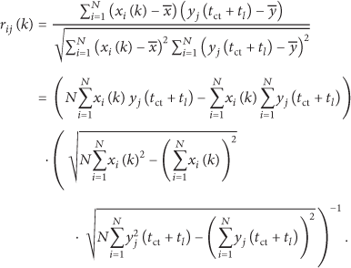
It means higher correlation if the absolute value of spatial and temporal correlation coefficient is closer to 1. Then information of the most m correlated road segments and corresponding time stamp will be chosen as extracted features, that is, six parameters ( ${\mathbf{F}}_{\mathbf{m}}$ , ${\mathbf{c}}_{\mathbf{m}}$ , ${\mathbf{\Delta }}_{\mathbf{m}\mathbf{x}}$ , ${\mathbf{d}}_{\mathbf{m}\mathbf{x}}$ , ${\mathbf{w}}_{\mathbf{m}}$ , ${\mathit{l}}_{\mathit{m}}$ ). ${\mathbf{F}}_{\mathbf{m}}$ , ${\mathbf{c}}_{\mathbf{m}}$ denote the average speed and the certain state of the $m_{\text{th}}$ road segment at the corresponding time stamp. ${\mathbf{\Delta }}_{\mathbf{m}\mathbf{x}}$ and ${\mathbf{d}}_{\mathbf{m}\mathbf{x}}$ denote the interval of the time stamp and geodistance between the predicted road segment and its $m_{\text{th}}$ most correlated road segment, respectively. ${\mathbf{w}}_{\mathbf{m}}$ and ${\mathit{l}}_{\mathit{m}}$ denote the width and length of the $m_{\text{th}}$ most correlated road segment.

Principle Component Analysis. After extracting features by correlation coefficient approach, Principle Component Analysis (PCA) is adopted to reduce data dimension and compress the data volume efficiently. The features of m most correlated road segments construct the original data matrix. Consider

$$\begin{array}{cc}& C={\left[c\left(\mathrm{1}\right)c\left(\mathrm{2}\right)\cdots c\left(\mathrm{6}\right)\right]}^T\in R^{\mathrm{6}\times m},\end{array}$$

(2)

where $c(i)=[c_1\left(i\right)c_2(i)\cdots c_m(i)]\in R^m$ . In order to overcome such problems as the disunity of the original data, the raw data is normalized as follows:

$$\begin{array}{cc}& x_j\left(i\right)=\frac{c_j\left(i\right)-e\left(c_j\right)}{\delta \left(c_j\right)}\hspace{1em}\forall i,j,\\ X={\left[x\left(1\right)x\left(2\right)\cdots x\left(6\right)\right]}^T\in R^{6\times m},\end{array}$$

(3)

where ${\delta }^{\mathrm{2}}\left(c_j\right)=\left(1/5\right){\sum }_i^6[c_j(i)-e(c_j){]}^2$ is the sample variance and $e(c_j)=\left(1/6\right){\sum }_{i=1}^6{c}_j(i)$ is the sample mean. Then the covariance matrix of traffic flow in road segments can be constructed as follows:

$$\begin{array}{cc}& S=\frac{1}{m-1}{\displaystyle \sum }_j\left(x_j-〈x〉\right){\left(x_j-〈x〉\right)}^T,\end{array}$$

(4)

where $〈x〉=(1/m){\sum }_j^{}{x}_j$ . All eigenvalues of the covariance matrix R are found through the matrix computationand the sequence is ${\lambda }_1\ge {\lambda }_2\ge \cdots \ge {\lambda }_6\ge 0$ .

As principle components contain most information, we only need to extract part of the main components. The contribution rate of each eigenvalue is

$$\begin{array}{cc}& \frac{{\lambda }_i}{{\sum }_{k=1}^6{\lambda }_k}=\frac{{\lambda }_i}{6}.\end{array}$$

(5)

The cumulative contribution rate of the preceding r principle components is computed as $\sum {\alpha }_r$ . When this contribution rate is larger than a constant value ψ, we only need to extract r principle components which can reflect main information of all variables. Consider

$$\begin{array}{cc}& {\displaystyle \sum }{\alpha }_r=\frac{{\sum }_{k=1}^r{\lambda }_k}{{\sum }_{k=1}^6{\lambda }_k}.\end{array}$$

(6)

Finally the sample can be projected on the selected r feature vectors and a $r\times m$ feature matrix is obtained for feature learning.

4.1.2. Feature Learning with RBM

The main idea of deep learning approach RBM in O-Sense is that a plenty of preextracted temporal-spatial traffic data are processed into informative low-dimensional features, and then these learned features are used to train an efficient classifier SVM.

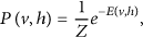
RBM is a generative stochastic neural network that can learn a probability distribution (e.g., $p(v,h)$ ) over the input set, which is good at reasoning about and predicting irregular and stochastic behavior in the traffic flow. As shown in Figure 3, RBM is in the shape of a bipartite graph with no intralayer connections. The hidden unit activations h (low-dimensional data) are mutually independent given the visible unit activations v; that is, when constraints are given on v, all hidden units are conditionally independent; that is, $p(h\hspace{0.17em}|\hspace{0.17em}v)=p(h_1\hspace{0.17em}|\hspace{0.17em}v)\cdots p(h_q\hspace{0.17em}|\hspace{0.17em}v)$ , and vice versa. Given visible layer v, hidden layer h can be obtained through $p(h\hspace{0.17em}|\hspace{0.17em}v)$ ; meanwhile the value of units is gained by getting the hidden units $p(v\hspace{0.17em}|\hspace{0.17em}h)$ . Through adjusting the parameters, the visible layer $v_1$ obtained from hidden layer can approximately equal the original input layer v. From this perspective, the outputs of hidden units are another representation of the visible units; namely, the original high-dimensional traffic information has been transformed into low-dimensional representative data.

Figure 3

Temporal-spatial feature deep learning model.

The standard type of RBM has binary-valued hidden and visible units and consists of a matrix of weights in which $w_{ij}$ denotes the connection weight between hidden unit $h_j$ and visible unit $v_i$ , $a_i$ denotes the bias of $v_i$ , and $b_j$ denotes the bias of $h_j$ . Given parameters $\theta =(w_{ij},a_i,b_j)$ , the energy of a configuration $(v,h)$ is defined as

$$\begin{array}{cc}& E\left(v,h;\theta \right)=-{\displaystyle \sum }_{i=\mathrm{1}}^{rm}{a}_i{v}_i-{\displaystyle \sum }_{j=\mathrm{1}}^q{b}_j{h}_j-{\displaystyle \sum }_{i=\mathrm{1}}^{rm}{\displaystyle \sum }_{j=\mathrm{1}}^q{h}_j{w}_{ij}{v}_i.\end{array}$$

(7)

This energy function is analogous to that of a Hopfield network [23]. As in general Boltzmann machines, probability distributions over hidden and visible vectors are defined in terms of the energy function. Consider

$$\begin{array}{cc}& P\left(v,h\right)=\frac{1}{Z}{e}^{-E\left(v,h\right)},\end{array}$$

(8)

where Z is a partition function defined as the sum of $e^{-E\left(v,h\right)}$ over all possible configurations. Similarly, the marginal probability of a visible vector of Booleans is the sum over all possible hidden layer configurations. Consider

$$\begin{array}{cc}& P\left(v\right)=\frac{1}{Z}{\displaystyle \sum }_h{e}^{-E\left(v,h\right)}.\end{array}$$

(9)

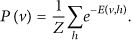
Then the probability under the condition that $h_j$ equals 1 and the probability under the condition that $v_i$ equals 1 are given as follows:

$$\begin{array}{cc}& P\left(h_j=1\hspace{0.17em}|\hspace{0.17em}v;\theta \right)=\sigma \left(b_j+{\displaystyle \sum }_{i=1}^{rm}{w}_{ij}{v}_i\right),\\ P\left(v_i=1\hspace{0.17em}|\hspace{0.17em}h;\theta \right)=\sigma \left(a_i+{\displaystyle \sum }_{j=1}^q{w}_{ij}{h}_j\right),\end{array}$$

(10)

where $\sigma (x)=1/(1+e^{-x})$ denotes the logistic sigmoid function and the parameters $\theta =(w_{ij},a_i,b_j)$ can be learned by gradient-based contrastive divergence algorithm [24].

4.1.3. Training a SVM Model

After input data is compressed by RBM, more representative features are extracted as the inputs of SVM for better classification effect. Through training a SVM classifier, we can get 5 classifications of traffic flow state and their probabilities construct a vector. Consider

$$\begin{array}{ll}P\left(t\right)& =\left[p\left(\text{state}=\text{Cg}\right),p\left(\text{state}=\text{Sl}\right),p\left(\text{state}=\text{Nm}\right),\right.\\ & \hspace{1em}\hspace{0.5em}\left.p\left(\text{state}=\text{Mo}\right),p\left(\text{state}=\text{Un}\right)\right].\end{array}$$

(11)

4.2. Temporally Related Supplementary Feature Learning

Observing from the data distribution, there are enough taxi GPS traces at day, which is, however, insufficient at midnight. When traffic information is insufficient at some certain times, the deep learning approach which only utilizes big data for traffic condition prediction cannot make enough effect [25]. Through supplementary feature learning, environmental information relevant to traffic condition for each road segment can be well taken into account and then make the prediction become more profound and accurate. This approach basically involves three main processes, environmental feature extraction, CRF real-time estimation, and sequence segments matching.

4.2.1. Environmental Feature Extraction

The traffic condition can be reflected by environmental information. Apparently, most of the road noise is emitted by vehicles. The observed patterns of noise can reflect under which traffic conditions it was produced [26, 27]. A high rainfall intensity also influences the traffic condition [28]. Owning to the reduced visibility and pavement friction, the effective travel times are greater than the mean travel time as expected. In addition, the rainfall intensity will also influence the travelers’ path choice. If the effective travel time on one path is less sensitive to the rainfall as compared to other paths, most travelers choose or switch to the path with the probability of a higher rainfall intensity. A high wind speed results in a more hazardous trip and travel times are longer and less reliable, which leads to some travelers deferring trips or cancelling them [29]. The impact of temperature and PM2.5 is not very clear, but a good traffic condition is more likely when the temperature is high and PM2.5 is low.

When there is little traffic information at midnight, environmental information especially road noise can well reflect traffic condition. Road noise is mainly affected by traffic flow at night, which is not the same as during the day that contains interference factors. Hence, the sparse period of traffic information especially at midnight is quite suitable for being supplied with environmental information.

We select some environmental features that related to the traffic, road noise, temperature, wind speed, PM2.5, and rainfall denoted by a 5-dimensional vector $E=[e_1,e_2,e_3,e_4,e_5]$ , where $e_i$ ( $i=\mathrm{1,2},\dots ,\mathrm{4,5}$ ) is the value of each feature.

4.2.2. CRF Real-Time Estimation

The characteristic mode and temporal evolution rule of the traffic flow state are investigated by using linear-chain CRF method [30], considering the supplementary features such as E of the predicted road segment.

A linear-chain CRF is a discriminative probability undirected graphical learning model. The advantage of CRFs over hidden Markov models (HMM) is the relaxation of the independent assumptions between features. HMM is necessarily local in nature because they are constrained to binary transition and emission feature functions, which forces each state to depend only on the current label and each label to depend only on the previous label; however, CRF can use more global features. Additionally, CRF can obtain the global optimal value with the global normalization of all features. Building the special case of a linear-chain CRF, features are restricted to depend on only the current and previous labels instead of arbitrary labels throughout.

As shown in Figure 4, an undirected graph G consists of two kinds of nodes. The white nodes $\mathbf{Y}=\{Y_1,Y_2,\dots ,Y_n\}$ represent traffic flow state variables at continuous time stamps, connected with supplementary features represented by blue nodes $\mathit{X}=\{X_1,X_2,\dots ,X_n\}$ , $X_t=\{E,t\}$ . Under observation sequence x, each random variable $Y_i$ obeys the Markov property; that is, $p(Y_v\hspace{0.17em}|\hspace{0.17em}X,Y_u,\hspace{0.17em}u\ne v)=p(Y_v\hspace{0.17em}|\hspace{0.17em}X,u~v)$   (u and v are adjacent nodes in G). Given observation sequence x at time t, the probability of each possible state for $Y_t$ is defined as follows:

$$\begin{array}{l}P\left(y\hspace{0.17em}|\hspace{0.17em}x,\lambda \right)\\ \hspace{1em}=\frac{\exp \left({\sum }_j{\lambda }_j{t}_j\left(y_{t-1},y_t,x,t\right)+{\sum }_k{\mu }_k{s}_k\left(y_t,x,t\right)\right)}{{\sum }_l\exp \left({\sum }_j{\lambda }_j{t}_j\left(y_{t-1},y_t,x,t\right)+{\sum }_k{\mu }_k{s}_k\left(y_t,x,t\right)\right)},\end{array}$$

(12)

where $t_j(y_{t-1},y_t,x,t)$ is the transfer feature function depending on the current time t and previous time $t-1$ , $s_k(y_t,x,t)$ represents the state feature function depending on the time t, and $y_t$ denotes the traffic flow state at time t. When meeting the known deterministic feature conditions, the value of $t_j$ or $s_k$ is 1, otherwise 0. ${\lambda }_j$ and ${\mu }_k$ can be estimated from training data.

Figure 4

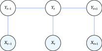
Temporally related feature learning CRF model.

Assuming that there is a bunch of samples which are independent of each other in training dataset $\text{Data}=\{x^{\left(z\right)},y^{(z)}\}$ , maximum likelihood estimation learning $p(y\hspace{0.17em}|\hspace{0.17em}x,\mathbf{\lambda })$ is used to learn the parameters λ by gradient descent algorithm [31]. Consider

$$\begin{array}{l}L\left(\lambda \right)={{\displaystyle \sum }}_z\begin{array}{l}\left[\log \frac{1}{{\sum }_y\exp \left[{\sum }_j{\lambda }_j{f}_j\left(y_{t-1},y_t,x,t\right)\right]}\phantom{{\displaystyle \sum }_j^{}{\lambda }_j{f}_j\left(y_{t-1},y_t,x,t\right)}\right.\end{array}\\ \hspace{1em}\hspace{0.17em}\hspace{1em}\hspace{1em}\hspace{1em}\hspace{1em}\hspace{0.5em}\left.+{{\displaystyle \sum }}_j{\lambda }_j{f}_j\left(y_{t-1},y_t,x,t\right)\right].\end{array}$$

(13)

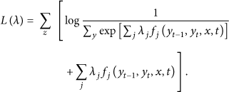
By setting $s_k(y_t,x,t)=s_k(y_{t-1},y_t,x,t)$ , two feature functions are unified into $f_j(y_{t-1},y_t,x,t)$ , which includes an observation sequence x, the time t, the current state $y_t$ , and the previous state $y_{t-1}$ . Assuming that there are $K_1$ transfer feature functions and $K_2$ state feature functions under the given deterministic feature conditions, $K=K_1+K_2$ , $f_j(y_{t-1},y_t,x,t)$ is represented as follows:

$$\begin{array}{l}{f}_j(y_{t-\mathrm{1}},y_t,x,t)\\ \hspace{1em}=\left\{\begin{array}{ll}{t}_j(y_{t-\mathrm{1}},y_t,x,t),\hfill & j=\mathrm{1,2},\dots ,K_{\mathrm{1}}\hfill \\ s_k(y_t,x,t),\hfill & j=K_{\mathrm{1}}+k;\hspace{0.17em}k=\mathrm{1,2},\dots ,K_{\mathrm{2}}.\hfill \end{array}\right.\end{array}$$

(14)

Assigning each feature function $f_j$ a weight ${\lambda }_j$ and given an observation sequence x,  (12) can be transformed as follows:

$$\begin{array}{ll}P\left(y\hspace{0.17em}|\hspace{0.17em}x,\lambda \right)& =\frac{\exp \left[p\left(y\hspace{0.17em}|\hspace{0.17em}x,\lambda \right)\right]}{{\sum }_y\exp \left[p\left(y\hspace{0.17em}|\hspace{0.17em}x,\lambda \right)\right]}\\ & =\frac{\exp \left[{\sum }_j{\lambda }_j{f}_j\left(y_{t-1},y_t,x,t\right)\right]}{{\sum }_y\exp \left[{\sum }_j{\lambda }_j{f}_j\left(y_{t-1},y_t,x,t\right)\right]}.\end{array}$$

(15)

Through the above equation, the probabilities of five possible states for $Y_t$ can be informally denoted as a five-dimensional vector. Consider

$$\begin{array}{ll}P\left(t\right)=& \left[p\left(y_t=\text{Cg}\right),p\left(y_t=\text{Sl}\right),p\left(y_t=\text{Nm}\right),\right.\\ & \hspace{0.5em}\left.p\left(y_t=\text{Mo}\right),p\left(y_t=\text{Un}\right)\right].\end{array}$$

(16)

4.2.3. Sequence Segments Matching

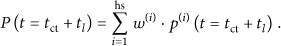
After applying CRF classifier to output a state vector of traffic flow at each time stamp, a state sequence segment can be obtained. Through finding similar state segments in history, we can obtain the state of traffic flow at the predicted time stamp according to the sequence matching with historical sequence segments. Since there may be no identical state sequence segments, measuring the similarity between sequence segments is necessary for sequence matching. Commonly used Euclidean distance is not suitable for the distance measurement of time-series sequences, which leads to the utilization of a nonlinear time alignment approach, namely, dynamic time warping (DTW).

In the process of state sequence segment matching, assuming that the current time is $t_{\text{ct}}$ , a traffic state sequence segment obtained from CRF classifier previouslyis represented as $S=(s_{t_{\text{ct}}-n·\Delta t+1},\dots ,s_{t_{\text{ct}}-\Delta t},s_{t_{\text{ct}}})$ and a predicted traffic state after time $t_l$ can be denoted as $s_{t_{\text{ct}}+t_l}$ . DTW-based segment matching algorithm, shown in Algorithm 2, is employed to procure adequate matching segments through measuring DTW distances between the given state sequence segment and historical segments $S^{*}=(s_{t_{\text{ct}}-n·\Delta t+1}^{*},\dots ,s_{t_{\text{ct}}-\Delta t}^{*},s_{t_{\text{ct}}}^{*})$ . In this algorithm, the predicted sequence segment is warped nonlinearly in time dimension to determine the similarity with historical segments. A constant thresholdε is defined to filter adequate traffic flow state segments in history according to the DTW distances which are less than the chosen threshold; that is, $\text{DT}{\text{W}}^{(i)}[t_{\text{ct}}][t_{\text{ct}}]\le \epsilon$ . Assuming there are hs adequate historical segments chosen through DTW-based segment matching algorithm, so we can get hs state probability vectors of 5-dimensional at the predicted time $t_{\text{ct}}+t_l$ , where $i_{\text{th}}$ probability vector is represented as

$$\begin{array}{l}{P}^{\left(i\right)}\left(t=t_{\text{ct}}+t_l\right)\\ \hspace{1em}=\left[p^{\left(i\right)}(s_t^{*}=\text{Cg}),p^{\left(i\right)}(s_t^{*}=\text{Sl}),p^{\left(i\right)}(s_t^{*}=\text{Nm}),\right.\\ \hspace{0.5em}\hspace{1em}\hspace{1em}\left.p^{\left(i\right)}\left(s_t^{*}=\text{Mo}\right),p^{\left(i\right)}\left(s_t^{*}=\text{Un}\right)\right].\end{array}$$

(17)

Algorithm 2: DTW-based segment matching algorithm.

Input: Historical segments:

    $$S^{\mathrm{*}(i)}=(s_{t_{\text{ct}}-n·\mathrm{\Delta }t+\mathrm{1}}^{\mathrm{*}(i)},\dots ,s_{t_{\text{ct}}-\mathrm{\Delta }t}^{\mathrm{*}(i)},s_{t_{\text{ct}}}^{\mathrm{*}(i)})\hspace{0.17em}\hspace{0.17em}(i=\mathit{1,2},\dots ,\text{hs})$$

   Predicted segment: $$S=(s_{t_{\text{ct}}-n·\mathrm{\Delta }t+\mathrm{1}},\dots ,s_{t_{\text{ct}}-\mathrm{\Delta }t},s_{t_{\text{ct}}})$$

Output: Adequate historical segments

Procedure:

(1) for  $$S^{*(i)}(\mathit{1}\le i\le \text{hs})$$

(2) for  $$t_{\text{ct}}-n\mathrm{\Delta }t+\mathit{1}<j,k\le t_{\text{ct}}$$ do

(3)   $${\text{Distance}}^{(i)}[j][k]==\mathit{0}$$ ;

(4)   $${\text{DTW}}^{(i)}[j][t_{\text{ct}}-n\mathrm{\Delta }t+\mathit{1}]==\inf$$ ;

(5)   $${\text{DTW}}^{(i)}[t_{\text{ct}}-n\mathrm{\Delta }t+\mathit{1}][k]==\inf$$ ;

(6) end;

(7)   $${\text{DTW}}^{(i)}[t_{\text{ct}}-n\mathrm{\Delta }t][t_{\text{ct}}-n\mathrm{\Delta }t]==\mathit{0}$$ ;

(8) for  $$t_{\text{ct}}-n\mathrm{\Delta }t+\mathit{1}<j,k\le t_{\text{ct}}$$ do

(9)   $${\text{Distance}}^{(i)}[j][k]=(s_{k-\mathit{1}}-{s_{j-\mathit{1}}}^{*\left(i\right)})*(s_{k-\mathit{1}}-{s_{j-\mathit{1}}}^{*(i)})$$

(10) end;

(11) for  $$t_{ct}-n\Delta t+\mathit{1}<j,k\le t_{ct}$$ do

(12)   $${\text{DTW}}^{(i)}[j][k]={\text{Distance}}^{(i)}[j][k]+\mathrm{Min}({\text{DTW}}^{(i)}[j-\mathit{1}][k-\mathit{1}]$$ ,

                       $${\text{DTW}}^{(i)}[j][k-\mathit{1}]$$ ,

                       $${\text{DTW}}^{(i)}[j-\mathit{1}][k])$$ ;

(13) end;

(14) if  $${\text{DTW}}^{(i)}[t_{\text{ct}}][t_{\text{ct}}]\le \epsilon$$

(15)  output  $$S^{*(i)}$$ ;

(16) end;

In the above formula, $S^{*(i)}$ is the $i_{\text{th}}$ adequate historical sequence segment and $P^{(i)}(s_t^{*}=s)$ ( $s\in \Omega$ ) represents the probabilities of five possible states at the predicted time $t_{\text{ct}}+t_l$ according to the $i_{\text{th}}$ historical segment $S^{*(i)}$ . Since $w^{(i)}$ is the weight of $i_{\text{th}}$ historical segment and can be calculated as

$$\begin{array}{cc}& w^{\left(i\right)}=\frac{\text{DT}{\text{W}}^{\left(i\right)}\left[t_{\text{ct}}\right]\left[t_{\text{ct}}\right]}{{\sum }_{i=1}^{\text{hs}}\text{DT}{\text{W}}^{\left(i\right)}\left[t_{\text{ct}}\right]\left[t_{\text{ct}}\right]},\end{array}$$

(18)

now, we can obtain the weighted vector at the predicted time t ( $t=t_{\text{ct}}+t_l$ ) as the final state result. Consider

$$\begin{array}{cc}& P\left(t=t_{\text{ct}}+t_l\right)={\displaystyle \sum }_{i=1}^{\text{hs}}\begin{array}{c}{w}^{\left(i\right)}·p^{\left(i\right)}\left(t=t_{\text{ct}}+t_l\right)\end{array}.\end{array}$$

(19)

4.3. Dynamic Weighted Classifier Fusion

During the daytime, the taxi traffic operation characteristics, which provide ample data of arterial roads, can objectively reflect real road traffic conditions of the city from a certain extent. However, applying supplementary information especially road noise to predict the traffic condition may be affected by some interference factors such as man-made noise during the daytime. In the early morning hours, pure road noise is more likely to better reflect the road traffic conditions, which makes it possible to achieve higher prediction accuracy than what is achieved by insufficient taxi GPS traces. Obviously, two different approaches have various prediction accuracies during different time in a day.

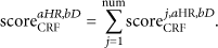
Comprehensively considering temporal-spatial features and supplementary features, a dynamic weighted classifier fusion is utilized to fuse two approaches to obtain a better result. We give scores to the prediction effects of two approaches every hour in one day, represented as $\text{scor}{\text{e}}_{\text{CRF}}^{a\text{HR},bD}$ and $\text{scor}{\text{e}}_{\text{DL}}^{a\text{HR},bD}$ , where $a\text{HR}$ represents the $a_{\text{th}}$ hour in one day and $bD$ denotes that $b_{\text{th}}$ day in history. Sampling num times per hour, we compare predicted state $s_t^j$ with actual state $s_t^{j,gt}$ at each sampling in one hour. $s_t^j$ represents the prediction result of $j_{\text{th}}$ sample in one hour that the time stamp t belongs to, while $s_t^{j,gt}$ is the corresponding ground truth, which is accurately defined in evaluation part. If $s_t^j$ is congruent with the ground truth, a positive value considering the probability of this state is assigned to the score; otherwise the score is assigned negative. Consider

$$\begin{array}{cc}& {\text{score}}_{\text{CRF}}^{j,a\text{HR},bD}=\left\{\begin{array}{cc}{P}_{\text{CRF}}^{\left(bD\right)}(s_t^{*}=s_t^j),\hfill & \text{if}\mathrm{\hspace{0.17em}\hspace{0.17em}}{s}_t^j\mathrm{\hspace{0.17em}\hspace{0.17em}}\text{is}\mathrm{\hspace{0.17em}\hspace{0.17em}}{s}_t^{j,gt}\hfill \\ -P_{\text{CRF}}^{\left(bD\right)}\left(s_t^{*}=s_t^j\right),\hfill & \text{if}\mathrm{\hspace{0.17em}\hspace{0.17em}}{s}_t^j\mathrm{\hspace{0.17em}\hspace{0.17em}}\text{is}\mathrm{\hspace{0.17em}\hspace{0.17em}}\text{not}\mathrm{\hspace{0.17em}\hspace{0.17em}}{s}_t^{j,gt},\hfill \end{array}\right.\end{array}$$

(20)

where $\text{scor}{\text{e}}_{\text{CRF}}^{j,a\text{HR},bD}$ represents the score of $j_{\text{th}}$ sample in the hour $a\text{HR}$ on day $bD$ . The sum of all scores in the hour $a\text{HR}$ of day $bD$ is calculated as follows:

$$\begin{array}{cc}& {\text{score}}_{\text{CRF}}^{aHR,bD}={\displaystyle \sum }_{j=\mathrm{1}}^{\text{num}}{\text{score}}_{\text{CRF}}^{j,a\text{HR},bD}.\end{array}$$

(21)

Similarly, we can also get the ${\text{score}}_{\text{DL}}^{j,a\text{HR},bD}$ and $\text{scor}{\text{e}}_{\text{DL}}^{a\text{HR},bD}$ as follows:

$$\begin{array}{cc}& {\text{score}}_{\text{DL}}^{j,a\text{HR},bD}=\left\{\begin{array}{cc}{P}_{\text{DL}}^{\left(bD\right)}(s_t^{*}=s_t^j),\hfill & \text{if}\mathrm{\hspace{0.17em}\hspace{0.17em}}{s}_t^j\mathrm{\hspace{0.17em}\hspace{0.17em}}\text{is}\mathrm{\hspace{0.17em}\hspace{0.17em}}{s}_t^{j,gt}\hfill \\ -P_{\text{DL}}^{\left(bD\right)}(s_t^{*}=s_t^j),\hfill & \text{if}\mathrm{\hspace{0.17em}\hspace{0.17em}}{s}_t^j\mathrm{\hspace{0.17em}\hspace{0.17em}}\text{is}\mathrm{\hspace{0.17em}\hspace{0.17em}}\text{not}\mathrm{\hspace{0.17em}\hspace{0.17em}}{s}_t^{j,gt},\hfill \end{array}\right.\\ {\text{score}}_{\text{DL}}^{a\text{HR},bD}={\displaystyle \sum }_{j=1}^{\text{num}}{\text{score}}_{\text{DL}}^{j,a\text{HR},bD}.\end{array}$$

(22)

When the expectation of scores in a given hour $a\text{HR}$ of all historical days is larger, the prediction will perform better. However, if the variance of scores in a given hour is larger, we will get worse prediction effect. Assuming that there are $ev$ days in the training dataset, prediction effects ${\alpha }_{a\text{HR}}$ and ${\beta }_{a\text{HR}}$ in two respective approaches considering expectations and variances at the corresponding hour of $ev$ days in the history can be defined as follows:

$$\begin{array}{c}{\alpha }_{a\text{HR}}=\frac{\overline{{\text{score}}_{\text{CRF}}^{a\text{HR}}}}{\mathrm{1}+\sqrt{{\sum }_{bD=1}^{ev}{\left({\text{score}}_{\text{CRF}}^{a\text{HR},bD}-\overline{{\text{score}}_{\text{CRF}}^{a\text{HR}}}\right)}^{\mathrm{2}}}},\\ {\beta }_{a\text{HR}}=\frac{\overline{{\text{score}}_{\text{DL}}^{a\text{HR}}}}{\mathrm{1}+\sqrt{{\sum }_{bD=1}^{ev}{\left({\text{score}}_{\text{DL}}^{a\text{HR},bD}-\overline{{\text{score}}_{\text{DL}}^{aHR}}\right)}^{\mathrm{2}}}},\end{array}$$

(23)

where $\overline{{\text{score}}_{\text{CRF}}^{a\text{HR}}}$ and $\overline{{\text{score}}_{\text{DL}}^{a\text{HR}}}$ denote the average values of scores in hour $a\text{HR}$ all $ev$ days in two different approaches.

In prediction process, we apply CRF approach and deep learning approach to learn features separately, generating two classifications with two probability vectors ( $P_{\text{CRF}}$ and $P_{\text{DL}}$ ) of 5-dimensional. The prediction result of O-Sense (donated as $P_{\text{OS}}$ ) can be calculated by fusing $P_{\text{CRF}}$ and $P_{\text{DL}}$ with respective weights at time t belonging to hour $a\text{HR}$ , which can be represented as follows:

$$\begin{array}{l}\mathrm{\hspace{0.17em}\hspace{0.17em}}{P}_{\text{OS}}=\frac{{\alpha }_{a\text{HR}}^{\mathrm{2}}}{{\alpha }_{a\text{HR}}^{\mathrm{2}}+{\beta }_{a\text{HR}}^{\mathrm{2}}}*P_{\text{CRF}}+\frac{{\beta }_{a\text{HR}}^{\mathrm{2}}}{{\alpha }_{a\text{HR}}^{\mathrm{2}}+{\beta }_{a\text{HR}}^{\mathrm{2}}}*P_{\text{DL}},\\ a\text{HR}=\left(\mathrm{1,2},\dots ,\mathrm{24}\right).\end{array}$$

(24)

5. Evaluations

5.1. Datasets

The datasets of Wuhan city are used for the evaluation of our traffic flow prediction and route computing. A representative region is selected to verify the validity of our mechanism. The following three available datasets are used.

• (1)

Taxi Trajectories: the trajectory datasets are generated by 30,000 taxis over a period of three months from January to March in 2013. Total distance of the dataset is about 450 million kilometers, and whole number of GPS points reaches 890 million. The interval sampling each time is 4.5 minutes with the distance of 500 meters between two consecutive points.

(2)

Road Network: the road network of Wuhan is adopted to perform the experiments. In Figure 5, a snapshot of the Wuchang district road network in Wuhan is displayed in the rush hour (5 pm).

(3)

Environmental data: from a public website, we collect environmental information which contains road noise, temperature, wind speed, PM2.5, and rainfall.

(4)

Ground truth: the actual traffic flow which can be known from camera sensor on the road is used as the ground truth to measure the prediction accuracy.

Figure 5

The road network of Wuchang district in Wuhan.

5.2. Performance

5.2.1. Evaluation of Temporal-Spatial Deep Learning Approach

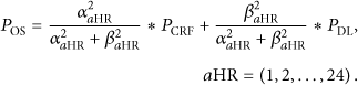
Several parameters need to be determined for utilizing a temporal-spatial deep learning approach. Since different network structures influence the forecast results obviously, the parameter effect needs to be tested. One of the most important problems in designing a neural network is to determine the size of the network. 128 nodes are chosen to be the number of input layer nodes. As the number of input layer node changes, different weighted mean accuracy (WMA) can be obtained. As shown in Figure 6, the best choice is 64 nodes based on our experiments. If there are more nodes, training the RBM model will increase both the redundancy and computational expense. However, fewer nodes cannot make full use of neural network to depict the characteristics of high-dimension, nonlinearity, and randomness in the transportation network.

Figure 6

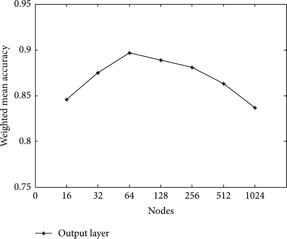
Effect of nodes in output layer.

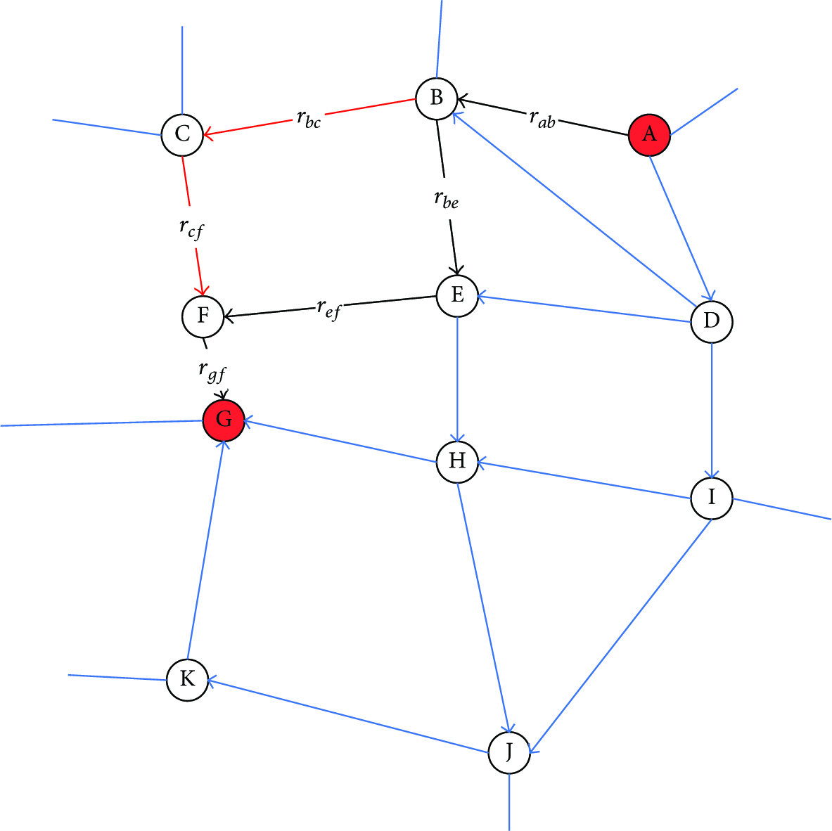
As shown in Figure 7, road segment $I_3$ chosen as the forecasted road segment denotes the traffic flow from upstream link F to downstream road I. As shown in Table 1, in order to predict the object traffic flow of $I_3(t_{\text{ct}}+T_{\text{predict}})$ at time $t_{\text{ct}}+T_{\text{predict}}$ , M ( $M=32$ can be calculated through number of input nodes in RBM) most closely correlated traffic flow with different time indexes are selected from all the following available traffic flows: $\{A_1(t_{\text{ct}}),A_1(t_{\text{ct}}-1),\dots ,A_1(t_{\text{ct}}-T)\}$ , $\{A_3(t_{\text{ct}}),A_3(t_{\text{ct}}-1),\dots ,A_3(t_{\text{ct}}-T)\},\dots$ , $\{I_3(t_{\text{ct}}),I_3(t_{\text{ct}}-1),\dots ,I_3(t_{\text{ct}}-T)\},\dots ,\{J_3(t_{\text{ct}}),J_3(t_{\text{ct}}-1),\dots ,J_3(t_{\text{ct}}-T)\}$ , and so forth. In this paper, we choose 5 min as the time unit and $T=20$ .

Table 1

Most correlated traffic flows with road segment $$I_{\mathit{3}}(t+T_{\text{predict}})$$ .

Traffic flow	Correlation
$$J_{\mathit{1}}(t)$$	0.971911
$$F_{\mathit{3}}(t)$$	0.967859
$$H_{\mathit{2}}(t)$$	0.967743
$$I_{\mathit{3}}(t)$$	0.967213
$$A_{\mathit{3}}(t-\mathit{1})$$	0.966754
$$A_{\mathit{3}}(t)$$	0.966512
$$B_{\mathit{4}}(t)$$	0.964985
$$A_{\mathit{4}}(t)$$	0.962859
$$D_{\mathit{1}}(t-\mathit{2})$$	0.962543
$$G_{\mathit{1}}(t-\mathit{1})$$	0.962211
$$D_{\mathit{1}}(t-\mathit{1})$$	0.961019
$$B_{\mathit{4}}(t-\mathit{1})$$	0.960609
$$G_{\mathit{1}}(t)$$	0.960312
$$A_{\mathit{4}}(t-\mathit{1})$$	0.959412
$$B_{\mathit{2}}(t-\mathit{1})$$	0.959289
$$F_{\mathit{3}}(t-\mathit{1})$$	0.957864
$$A_{\mathit{3}}(t-\mathit{2})$$	0.957535
$$H_{\mathit{3}}(t)$$	0.957198
$$B_{\mathit{2}}(t)$$	0.955938
$$A_{\mathit{1}}(t)$$	0.955543
$$E_{\mathit{1}}(t-\mathit{1})$$	0.954375
$$A_{\mathit{1}}(t-\mathit{2})$$	0.954102
$$G_{\mathit{3}}(t-\mathit{1})$$	0.946793
$$C_{\mathit{2}}(t-\mathit{1})$$	0.946776
$$H_{\mathit{4}}(t-\mathit{1})$$	0.944312
$$B_{\mathit{2}}(t-\mathit{2})$$	0.944023
$$J_{\mathit{2}}(t-\mathit{1})$$	0.941005
$$C_{\mathit{2}}(t)$$	0.926284
$$D_{\mathit{3}}(t-\mathit{2})$$	0.924927
$$G_{\mathit{3}}(t-\mathit{3})$$	0.919505
$$F_{\mathit{1}}(t-\mathit{1})$$	0.918812
$$C_{\mathit{1}}(t-\mathit{2})$$	0.902242

Figure 7

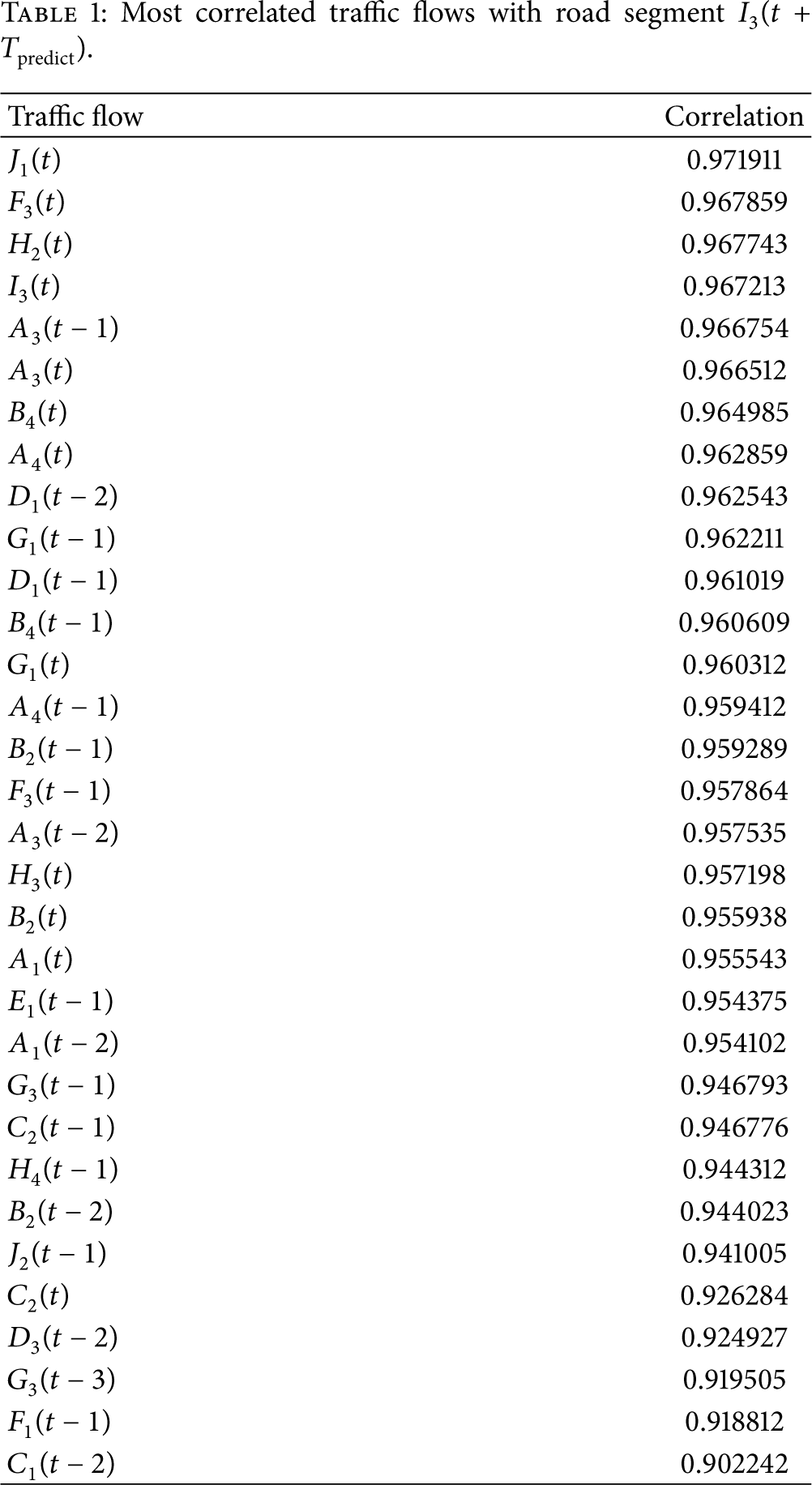
Illustration of road network segment.

In the PCA approach, we choose ψ as 95 percent and 6 eigenvalues of the covariance matrix can be obtained as shown in Table 2.

Table 2

Eigenvalue and contribution rate of the covariance matrix.

Eigenvalue	Contribution rate
2.2928	58.03%
0.8010	20.27%
0.6322	16.00%
0.1594	4.03%
0.0406	1.03%
0.0250	0.63%

After computing the cumulative contribution rate, we find that the cumulative contribution rate of the previous four principle components has achieved 98.33%. Hence, the previous four principle components can be considered to represent all information. The principle component structure of traffic flow is shown in Table 3.

Table 3

Principle component structure of traffic flow.

	Principle component
	1	2	3	4	5	6
$${\mathit{F}}_{\mathit{m}}$$	−0.0072	−0.0116	−0.0631	−0.2166	0.0764	−0.7433
$${\mathit{c}}_{\mathit{m}}$$	0.2076	−0.7524	−0.5373	0.2606	0.1545	−0.0683
$${\mathbf{\Delta }}_{\mathit{m}\mathit{x}}$$	0.2358	−0.4925	0.3296	−0.5935	−0.4530	0.1713
$${\mathit{d}}_{\mathit{m}\mathit{x}}$$	0.3975	−0.1156	0.5612	−0.0020	0.5919	−0.2532
$${\mathit{w}}_{\mathit{m}}$$	0.5540	0.0862	0.1869	0.4959	−0.1112	0.2889
$${\mathit{l}}_{\mathit{m}}$$	0.4671	0.2517	−0.1530	0.1169	−0.5413	−0.4488

To express the predicted state and its probability more clearly, we define five numbers for each state; for example, $\Omega =\{\text{congesting}\mathrm{\hspace{0.17em}\hspace{0.17em}}(\text{Cg})=\mathrm{1},\text{slow}\mathrm{\hspace{0.17em}\hspace{0.17em}}(\text{Sl})=\mathrm{2},\text{normal}\mathrm{\hspace{0.17em}\hspace{0.17em}}(\text{Nm})=\mathrm{3},\text{moderate}\mathrm{\hspace{0.17em}\hspace{0.17em}}(\text{Md})=\mathrm{4},\text{unimpeded}\mathrm{\hspace{0.17em}\hspace{0.17em}}(\text{Un})=\mathrm{5}\}$ . A road segment state is valued as the state number ${n^t}_r$ of the road segment r at the time stamp t. When a road segment traffic flow state is predicted as the state ${n^t}_r$ with the probability p, the predicted state value of the road segment is defined as ${n^t}_r\mathrm{\hspace{0.17em}\hspace{0.17em}}-1+p$ ; for example, when the predicted state of a road segment is Sl and the corresponding probability is 0.9 generated by deep learning approach, then the deep learning-based predicted state value is 1.9.

Figure 8 shows the traffic state prediction of deep learning approach with prediction time $\phi =15$  min. There are two time slots (about 8 am and 6 pm) where the prediction values are more close to the actual values. It can be inferred that, in the rush hours, there are sufficient taxi trajectories to learn the states of traffic flow and produce a more accurate prediction. Temporal-spatial deep learning approach can effectively extract the temporal-spatial features of high-dimensional, nonlinear, and random traffic flow. However, due to the lack of the sufficient taxi GPS traces, the traffic prediction accuracy in the early morning hours (from 1:00 am to 5:00 am) is significantly lower than that during the daytime. With the increase of the vehicles at 6 am, the prediction accuracy improves gradually. It can be seen that the deep learning approach cannot train an effective network to extract features due to the sparsity problem of data.

Figure 8

Traffic state prediction of temporal-spatial deep learning.

5.2.2. Evaluation of Temporally Related CRF Approach

Figure 9 demonstrates the prediction result of temporally related CRF approach with the prediction time $\phi =15$  min. According to the calculation, the prediction precision of CRF approach is nearly 0.75. Comparing the results of two approaches to predict separately in Figures 8 and 9, it can be inferred that the effect of deep learning approach is much better than CRF approach in most cases. However, temporally related CRF approach has better prediction effect on compensating for sparse data in deep learning approach. It takes full advantage of supplementary information especially road noise that provides effective information to improve the prediction accuracy when in the midnight.

Figure 9

Traffic state prediction of temporally related CRF approach.

5.2.3. Evaluation of Dynamic Weighted Classifier Fusion

In the following experiments, Figure 10 presents the expectations and the standard deviations of scores in the same hour varied in these two approaches. Two observations can be found in Figure 10(a). First, deep learning approach in the daytime has good performance using ample temporal-spatial traffic features. Second, the performance of CRF is higher when there is sparse data in the traffic network. As shown in Figure 10(b), CRF approach performs unstably in daytime on the account of the supplementary features such as road noise mainly caused by many active sources rather than just the vehicles in daytime.

Figure 10

Expectations and standard deviations of two approaches.

The dynamic weights of two different approaches in the same hour of one day are showed in Figure 11, which reveals that we can make more use of the advantages of two classifiers through fusing two approaches with the variety of time. Figure 12 presents better results obtained by fusion in different time of one day. For example, between 1 to 5 am in the morning, due to the sparse data in the traffic network, deep learning approach may have a low degree of recognition. However, CRF can obtain higher prediction precision during the period of time by extracting temporally related supplementary features. Hence, more accurate results can be gained by O-Sense which combines two approaches.

Figure 11

Dynamic weights of two approaches.

Figure 12

Traffic state prediction of O-Sense.

Figure 13 shows the precision, the recall, and the F1-measure of three approaches. As is shown in Figures 13(a) and 13(b), under the same prediction time, O-Sense can obtain 8% higher precision and recall than existing deep learning approaches. In Figure 13(c), the F1-measure, which considers both the precision and the recall, also reveals that O-Sense can obtain high accuracy. O-Sense comprehensively uses temporal-spatial traffic flow information and temporally related supplementary features in the traffic network. We can conclude that the effect of O-Sense is closer to the deep learning approach. Moreover, combining temporally related supplementary features used by CRF approach to overcome the problem of sparse data in deep learning, the prediction result of O-Sense can be further improved.

Figure 13

Study on three different approaches.

5.2.4. Evaluation of Online Route Computing

As is shown in Figure 14, two routes are selected to evaluate the performance of our mechanism. Route 1 starts from the Wuhan University to Hankou Railway Station and route 2 starts from Wuhan University to Guangda Masion. Route 1 has longer path length and costs much more time for travel than that of route 2, which can be seen in Figure 4. Comparing Figures 14(a) and 14(b), there are several observations as follows: Firstly, the traffic conditions almost remain unchanged at about 6 am and 12 am on route 1 and route 2. O-Sense and STR can both relatively accurately estimate the travel cost of the routes at that time. Secondly, the prediction performance of O-Sense is much better than STR in the time period containing different traffic conditions on route 1 (about 8 am and 4:30 pm). It can be inferred that starting at 8 am in the morning, driving on route 1 needs more than one hour to complete the whole path. The traffic condition of route 1 varies from congestion to slow then to normal. Hence, the total travel cost of the whole route depends on the real-time traffic condition of road segments when the user actually drives on them. Nevertheless, STR approach considers that the traffic conditions of road segments are always the same as their initial traffic condition at the departure time. It leads to the estimation that the travel cost by STR approach is much longer than the ground truth. The situation is similar as at 4:30 pm from that at 8 am, which can be seen as the estimated travel cost by STR is much shorter than ground truth. It can be inferred that the traffic condition on route 1 becomes congested after driving for about 30 minutes. The actual travel cost of the remaining path is much longer than that computed by the initial condition of each road segment in STR approach. Thirdly, route 2 takes less time than route 1 and the traffic conditions in that time period do not change too much; hence the STR performs better effects on route 2 at about 8 am and 4:30 pm.

Figure 14

Travel cost of two routes at different time.

Figure 15 shows the variation of driving speed at different places when the participant drives along route 1. STR keeps the speed of each road segment the same as that of the starting time for its static estimation policy, while O-Sense can estimate the real-time speeds for all the places on the route based on the predicted arrival time. When the user drives from the downtown area at 8 am, the traffic condition is congested. After the user drives about 4/6 distance of the whole path, the traffic flow shows high variation over time and traffic condition on current road segment becomes unimpeded. The traffic condition can be estimated by both STR and O-Sense on account of the rush hour at the beginning of traveling. Nevertheless, with the driving distance increasing, the traffic condition of the driving area becomes unblocked. Owning to the online traffic condition prediction of current road segment, O-Sense can perceive this variation and estimate the travel cost more accurately.

Figure 15

The speed after different travel distance at 8 am.

6. Conclusions

This paper proposes an online-traffic-prediction based route finding mechanism, namely, O-Sense, for fastest route finding with large scale taxi GPS traces and environmental information. In O-Sense, a temporal-spatial deep learning approach with preprocessed traffic-related features can effectively extract nonlinear, random, and high-dimensional characteristics from the traffic flow changes. Utilizing environment features as supplementary, CRF classifier can further reflect the dynamic patterns in the transportation network. A dynamic weighted classifier fusion approach is used to obtain a better prediction result, which helps to find the fastest route based on online route computing. We adopt trajectory datasets generated by 30,000 taxis over a period of three months in Wuhan to evaluate our approach. The experiment results showed that O-Sense can improve the travel cost estimation accuracy effectively.